
Abstract
Antibodies play an important role in the immune system by binding to molecules called antigens at their respective epitopes. These interfaces or epitopes are structural entities determined by the interactions between an antibody and an antigen, making them ideal systems to analyze by using docking programs. Since the advent of high-throughput antibody sequencing, the ability to perform epitope mapping using only the sequence of the antibody has become a high priority. ClusPro, a leading protein–protein docking server, together with its template-based modeling version, ClusPro-TBM, have been re-purposed to map epitopes for specific antibody–antigen interactions by using the Antibody Epitope Mapping server (AbEMap). ClusPro-AbEMap offers three different modes for users depending on the information available on the antibody as follows: (i) X-ray structure, (ii) computational/predicted model of the structure or (iii) only the amino acid sequence. The AbEMap server presents a likelihood score for each antigen residue of being part of the epitope. We provide detailed information on the server’s capabilities for the three options and discuss how to obtain the best results. In light of the recent introduction of AlphaFold2 (AF2), we also show how one of the modes allows users to use their AF2-generated antibody models as input. The protocol describes the relative advantages of the server compared to other epitope-mapping tools, its limitations and potential areas of improvement. The server may take 45–90 min depending on the size of the proteins.
Introduction
Antibodies form one of the key arms of the adaptive immune system in vertebrates. They target solvent-exposed proteins called antigens on the surfaces of pathogens. After recognition and contact, the antibodies mediate the humoral immune response to the attached pathogen1. The diversity and specificity of antibodies are the reason why harnessing their unique features is paramount in the pharmaceutical industry. Understanding and accurately predicting atomic-level details of the antibody–antigen interface are crucial for utilizing antibodies2. Finding the antigen residues in the interface, henceforth called ‘epitope mapping’, can be useful for the design of monoclonal antibodies3, for developing vaccines4 and for investigating immune responses5.
The development of methods for predicting antibody–antigen interactions and for antibody-based drug discovery was traditionally handicapped by the difficulty of obtaining high numbers of antibody sequences. However, because of advances in high-throughput single-cell and variable-diversity-joining sequencing of the B-cell receptor repertoire6,7, the availability of antibody sequences is no longer an issue in the race toward developing antibody-based drugs. Fast and accurate prediction of the epitopes for these antibody targets has become the new bottleneck8. Currently, epitope mapping efforts are dominated by experimental techniques such as X-ray crystallography, mutagenesis (e.g., alanine scanning) and phage display. X-ray crystallography is laborious and expensive, whereas mutagenesis and phage display generally do not provide atomic-level details9. Importantly, none of these experimental methods can be used in a high-throughput manner. In view of these limitations, substantial efforts have been devoted to the development of computational epitope-mapping methods10,11,12,13,14,15. However, epitope prediction for a given antigen and a given antibody is a difficult computational problem that requires further development to improve the accuracy and reliability of the predictions16. Part of the difficulty is due to the paucity of nonredundant structural data on antibody–antigen interactions, because, as reported by Jespersen et al. in 2017, <25% of the antibody–antigen complexes found in the Protein Data Bank (PDB) are unique when taking a 70% sequence identity threshold cutoff for the antigen17.
The challenge of epitope mapping can be partially addressed by finding residues on the antigen’s surface that are most likely to interact with a generic antibody (as opposed to a specific antibody)10,12,17,18. Some examples of such an approach are implemented in the servers Spatial Epitope Prediction for Protein Antigens (SEPPA)10,12 and BEpro (formerly known as PEPITO)18. SEPPA uses a logistic regression algorithm with features such as antigen residue surface accessibility and propensity for unit-triangle patches (three residue groups on the antigen’s surface) among other factors to score the surface residues10,11,12. BEpro adds an amino-acid propensity scale and side-chain orientations besides other features18. Despite the achievements of the antibody-agnostic approach, it is crucial to highlight that epitopes are, by definition, relational entities and that epitope mapping ought to be antibody specific. This is evidenced by several antigens with particular affinities to different antibodies at different interfaces. A well-studied example is hen egg lysozyme, which is crystallized with four different antibodies in the PDB structures 1BVK, 1DQJ, 2I25 and 1MLC, with little overlap19,20,21,22. Therefore, consideration of both the antibody and the antigen in epitope mapping not only is appropriate but generally also increases the accuracy because more information can be gleaned from the antibody side4.
This relational nature of epitopes makes it especially attractive to approach the epitope-mapping problem by using docking, which is a computational method that conventionally predicts the binding mode of two biological units23. One fairly successful example of such methods is ClusPro24,25,26. ClusPro is a webserver that directly docks two interacting proteins when given their X-ray structures. The server is freely available to those in nonprofit organizations and is used by over 20,000 scientists worldwide. It runs on a rigid-body docking program called ‘PIPER’, which uses a fast-Fourier transform (FFT) correlation approach27. The interaction energy, which is composed of van der Waals (vdW) energy terms (repulsive and attractive), electrostatic energy (Coulombic and Born approximations) and a structure-based pairwise statistical potential, is used for ranking the docked models. In 2012, a special antibody–antigen version of the pairwise statistical potential was introduced, vastly improving antibody–antigen docking accuracy28. In a recent comparative study, ClusPro was reported as the best server for antibody–antigen docking29. Hua et al. used the top 30 models predicted by ClusPro and combined it with site-directed mutagenesis to localize epitopes on several case studies successfully9. However, they also stated that docking alone or machine learning–based methods did not provide unique epitope positions and had to be followed by experiments9. Krawczyk and colleagues used a docking method in their epitope-mapping server EpiPred30. They used ZDOCK, an FFT-based rigid-body docking method to generate models to score putative epitope patches determined by geometric fitting30,31. More recently, Sikora and colleagues performed rigid-body Monte Carlo docking of monoclonal antibody against glycosulated SARS-CoV2 spike protein configurations to check for the accessibility of potential epitope candidates32.
One challenge that both Krawczyk et al. and Hua et al. faced, when using the EpiPred and ClusPro servers, respectively, was the servers’ inability to work with sequences9,30. Working with sequences requires a separate modeling step (which is not offered by EpiPred and ClusPro) if the antibody’s X-ray structure is not available. However, as mentioned above, antibody sequencing has made major advances over the past few years, whereas the technology for determining the X-ray structure of antibodies has not substantially improved33,34. This limitation implies that epitope-mapping tools should ideally include the ability to model the antibodies from their sequences in addition to mapping the epitopes on the given antigen structure. As a response to this need, we present in this work an end-to-end epitope-mapping server based on ClusPro’s docking protocol, ClusPro Antibody-based Epitope Mapping (ClusPro-AbEMap), that offers template-based modeling of the antibody if an X-ray structure is not available. The ClusPro-AbEMap server (https://abemap.cluspro.org/) integrates our template-based modeling method35 and antigen–antibody contact prediction via docking36,37 to identify the epitope of a given antigen structure from an antibody sequence or X-ray structure.
If the X-ray structure of the antibody is known, thousands of low-energy antibody–antigen models predicted by PIPER—the rigid-body docking program on which ClusPro is based—are used to score the antigen surface residues. If the X-ray structure of the antibody is unknown, AbEMap builds multiple homology models of the antibody that are used for docking instead. The consensus of the docked complexes based on all the antibody models and antigen structure templates is used to score the antigen residues. For the model antibodies, special care should be taken not to penalize possible clashes, by reducing the weight of the vdW component of the interaction energy. Although epitope prediction remains a difficult computational problem, and clearly more method development is required, we present the protocol for AbEMap, which performs better than the popular peer servers SEPPA, BEpro and EpiPred38.
Finally, we explore the potential use of deep neural network–based method AlphaFold2 for antibody structure prediction as well as epitope mapping. It has been demonstrated in the CASP14 experiment and now is well established that AlphaFold2 substantially improves the accuracy of predicting the structure of most monomeric proteins39,40,41. We show that AlphaFold2-modeled antibodies perform nearly as well as our ensemble of template-based models. However, according to our results, using the linker-based approach to predicting protein–protein interactions, which was recently proposed by several groups42,43,44,45, does not improve the accuracy of AbEMap in finding antibody epitopes.
The AbEMap algorithm and server overview
The server has two modes of running: the first requires an antibody structure as input, which can be an X-ray structure or a precomputed homology model, and the second can perform epitope prediction starting from the amino acid sequence of the antibody, assuming that appropriate antibody homologous structures are available in the PDB. The antigen structure is assumed to be known in both modes. The protocol for performing the second mode includes both homology modeling and docking (Fig. 1a–f). It builds multiple (if applicable) antibody models that form an ensemble. Once structures are available for both antibody and antigen, their mutual conformational space is sampled by using PIPER26, the docking engine of the ClusPro server, and the 1,000 lowest-energy complex poses are identified. When ClusPro is used for protein–protein docking, the 1,000 structures are clustered, and the centers of the most-populated clusters are selected as models of the complex. However, for epitope prediction, the 1,000 structures are instead used to calculate the frequency of each antigen surface atom’s occurrence in the antibody–antigen interface. As will be shown, to map an epitope, AbEMap defines the atomic epitope likelihood score as the Boltzmann weighted atomic interface occurrence frequency averaged over the ensemble of antibody structures.

a, The user inputs the solved crystal structure of the antigen (shown as PyMOL stick figures in purple) and the antibody sequence (shown as purple text) (if the structure is unavailable). b, The antibody sequence is used to find close homologs by using BLAST for each of its heavy (H) and light (L) chains. A sample multiple sequence alignment of close homologs is shown for the monoclonal murine antibody 1FGN. L1 and H1 (green), L2 and H2 (blue) and L3 and H3 (red) regions of the complementarity-determining regions are highlighted. The list of homologs is filtered by using sequence identity and sequence similarity of L3 and H3 regions to the query sequence. c, The structures for the selected sequences are modeled individually by using MODELLER. Aligned regions of the backbone are copied from the template, whereas non-aligned regions are modeled. d, The residues with the highest likelihood of being in the epitope are highlighted in red on the results page of the server. e, Billions of antibody–antigen complex conformations are generated by PIPER for the given antibody structure or for each antibody model. The antibody is shown as a translucent cartoon, and the antigen is shown as a cyan surface. f, The bar plot shows the number of poses in the top 100 models generated by PIPER that are within different root mean square deviation (RMSD) thresholds. For example, three models (in the top 100) have RMSD ≤2 Å, and 21 models have RMSD between 10 and 12 Å. g, As examples of visualizing the results, modeled murine anti-tissue factor (PDB ID 1FGN) and tissue factor (PDB ID 1TFH) are shown as surfaces with residues colored from blue to red on the basis of increasing predicted epitope likelihood score. 19 of the 26 epitope residues are in the 30 top-ranked residues. h, Modeled humanized Fab D3h44 (PDB ID 1JPT) and tissue factor (PDB ID 1TFH) shown as surfaces with residues colored from purple to gold on the basis of increasing predicted epitope likelihood score. 20 of the 24 epitope residues are in the 30 top-ranked residues. i, Modeled anti-CCL2 neutralizing antibody (PDB ID 4DN3) and monocyte chemoattractant protein (1DOL) are shown as surfaces with residues colored from orange to green on the basis of a decreasing predicted epitope likelihood score. All 14 of the 14 epitope residues are in the 30 top-ranked residues. j, Modeled anti-shh chimera Fab fragment (PDB ID 3MXV) and sonic hedgehog N-terminal domain (PDB ID 3M1N) shown as surfaces with residues colored from yellow to red on the basis of increasing predicted epitope likelihood score. 15 of the 24 epitope residues are in the 30 top-ranked residues. k, The distribution of the area under the receiver operating characteristic curve (ROC AUC) scores of 28 unbound antibody–antigen complexes for two of the top epitope-predicting servers (SEPPA and BEpro) are compared to that of AbEMap. AbEMap outperforms both in terms of the average (red dot), median (middle line) and 25th and 75th quartiles. l, The F1 and MCC scores of three different methods are compared for model antibodies when only homologs with <80% sequence identity are used as templates. ClusPro AbEMap takes the ensemble average residue scores from 5 to 10 of the best homologs, and EpiPred is used for epitope prediction with the best model antibody. AbEMap outperforms EpiPred before and after ensemble averaging of the likelihood scores.
When given only amino acid sequences of the heavy and light chains of the antibody in the more general second mode, ClusPro-AbEMap starts with a BLAST search for homologous structures in the PDB (Fig. 1b). It restricts sequence identity to be above 20% and e-value below 1 × 10–40, but in case no templates are found, the e-value threshold is increased to 1 × 10–20. Once the search is complete, only templates with both heavy and light chains that meet the sequence constraints are retained. The resulting templates are then ranked on the basis of both sequence identity and sequence similarity of CDR3s in the heavy and light chains. For complementarity-determining region (CDR) detection, we use the same tools as in the ClusPro server46. We take the five highest-ranked structures based on CDR3 sequence identity and the five highest-ranked structures based on CDR3 sequence similarity and use the union of the two sets as antibody templates. If the CDRs of the antibody cannot be identified, or if there is no CDR (as in single-domain antigen receptors), then the five top candidates ranked by the global sequence identity are selected. The second step is constructing homology models of the antibody on the basis of the selected templates (Fig. 1c). MODELLER tools47 are used to realign the antibody sequences, taking into account the template structural information. The program models the backbone atoms of the non-aligned residues and all side chains, while the backbone atoms of the aligned residues are kept fixed at the template coordinates. The single best model proposed by MODELLER for each template is retained for the next step in the epitope-mapping process; thus, AbeMap generally retains multiple antibody models.
When given an antibody X-ray structure or antibody models that have been already constructed, the next step of AbEMap is global antibody–antigen docking by the PIPER program27 that directly docks two protein structures (Fig. 1e). PIPER uses the FFT correlation approach48, which represents the interaction energy of the complex as a weighted sum of correlations between the fixed receptor and rotationally and translationally mobile ligand grids. Together with the FFT method, this representation makes exhaustive conformational sampling of the six-dimensional energy landscape computationally feasible. The standard level of discretization used in PIPER is 70,000 rotations from the Sukharev quasi-uniform grid sequence49 (approximately 5 degrees by Euler angular step) and a translational grid step size of 1 Å. The energy function E includes terms representing repulsive and attractive components of the vdW energy (denoted as Erep and Eattr, respectively), a Columbic term describing the electrostatic interaction energy (ECoul), a generalized Born-type polar solvation energy term (EBorn) and another solvation term based on the structure-based statistical potential EDARS based on the Decoys As the Reference State (DARS) approach50. A special antibody–antigen asymmetric version of the DARS potential has been developed, significantly improving ClusPro’s antibody–antigen docking accuracy28. This antibody–antigen–specific potential takes advantage of the fact that aromatic residues dominate the paratope but not necessarily the epitope, whereas the epitope generally has a higher level of hydrophobicity than the paratope.
To sample antibody–antigen interaction, the known antigen structure is docked to either the known antibody X-ray structure or the ensemble of antibody homology models obtained in the previous step from the antibody sequence data. Following our recently published protocol46, we mask all antibody residues except for CDRs. The server shows results for the energy function currently used in ClusPro for antibody–antigen docking (E = 0.5 Erep − 0.2 Eattr + 300 ECoul + 30 EBorn + 0.2 EDARS). If the input is a computationally predicted or homology-modeled structure or just the antibody sequence, then results for two additional weight sets are provided for the user as default: the option ‘No vdW’, which means that the weights for both vdW contributions are zeroed out, and the option ‘Reduced attractive vdW’, which implies that the weight for the attractive vdW term Eattr is halved. These additional weight sets avoid penalizing possible steric clashes. However, it should be noted that the commonly used maximum repulsive and minimum attractive vdW thresholds are still in place for all coefficients. Reducing the vdW potential’s weights notably increased epitope prediction accuracy when using the AbEMap protocol when only the sequence of the antibody or homology-modeled structure was given (Supplementary Fig. 1). As in the ClusPro server, the best-scored pose per rotation is retained, resulting in a total of up to 70,000 docked poses for further analysis.
Once the PIPER docking poses and energies are obtained for the antibody structure or for each antibody model i in the ensemble of homology models (which can include one or several models, depending on the number of suitable templates), the top 1,000 lowest-energy poses are selected, and for each such pose j, the number lij of antigen surface atoms51 that are in contact with the corresponding antibody is counted. More precisely, any heavy atom on the antigen surface found to be within the 5-Å threshold from any of the antibody surface heavy atoms is considered to be in contact with the antibody. For each antigen atom on the interface, we calculate a Boltzmann-weighted normalized contact ‘occurrence’ as follows:
where εij and εio are the jth and the best PIPER energy scores of the ith antibody structure in the ensemble, and a value of 100 was used for T (‘temperature’) to scale the relative energy scores. After summing the atomic contributions shown above over j (the docked structures) and averaging over i (the different antibody models), an epitope likelihood score that indicates how often the atom participates in the antibody–antigen interface of low-energy models predicted by PIPER is obtained. The total number of considered docked structures and the ‘temperature’ factor were optimally selected by using the receiver operating characteristic (ROC) AUC score obtained from the likelihood scores of each residue (area under the ROC curve; this score is described in more detail below in Performance measures). The top 1,000 lowest-energy poses and a T value of 100 give the best results (Supplementary Fig. 2). Because PIPER generally increases the number of docked structures around the native interface, it is expected and observed that atoms predicted to be in the epitope more frequently by the docked structures are more likely to be in the true epitope. This likelihood score is shown as the B-factor value in the final PDB file given to the user (Fig. 1d), and it helps to visually highlight plausible epitope regions. For evaluating epitope prediction accuracy, we convert the atom likelihoods to residue likelihoods by summing up the atomic contributions for each residue. Although adding atomic likelihood values implies that bigger residues with more surface-accessible atoms are scored better, the residue likelihood values are not corrected for size, and hence this bias may have to be accounted for by the user.
Protein datasets used for testing AbEMap
A set of 40 antibody–antigen complexes found in the widely accepted protein–protein docking benchmark version 5.0 (BM5)52 from the Weng laboratory was used to test our protocol (Figs. 1–3). To ensure non-redundancy, the authors selected an antibody–antigen complex only if the antigen was not in the same Structural Classification of Proteins53 family, and it did not share more than 80% of the interface residues with another52. The BM5 set contains 12 antibody–antigen complexes with the antibody crystallized only in complex with the respective antigen but not on its own (termed ‘unbound-bound targets’). For the other 28 complexes, the X-ray structure of the antibody has been determined both on its own and in complex with the antigen (termed ‘unbound-unbound targets’). In both cases, the antigen was independently crystallized in addition to its form in a complex with the respective antibodies. We compared the performance of AbEMap to that of SEPPA, BEpro and EpiPred by using this set of antibody–antigen complexes. However, EpiPred did not work for one of the unbound targets (PDB ID 2I25), most likely because it contains a single-chain shark antigen receptor without any CDR rather than a traditional antibody. Therefore, the target 2I25 was excluded from figures that compare AbEMap with EpiPred. In addition, we wanted to test the protocol on the 23 antibody–antigen complexes that were recently added to the docking benchmark set (denoted ‘BM5.5’)29. However, AbEMap was unable to provide antibody models for two of the complexes, and hence our discussion is restricted to the remaining 21 targets.

F1 and MCC scores for ClusPro-AbEMap, SEPPA, EpiPred and BEpro at different cutoff thresholds when the antigen residues are ranked by the obtained scores. The measures are averaged over the 28 complexes. The AbEMap results are slightly better than the ones obtained by SEPPA and substantially better than the ones obtained by BEPro and EpiPred.

a, The complex of birch pollen Bet V1 (blue surface) with the bound monoclonal antibody (magenta), PDB ID 1FSK. The true epitope residues are highlighted in red, and three of the homology models of the antibody are shown in green. The CDR3 of the heavy chain on the native antibody is highlighted in cyan. b, The integrin alpha-L 1 domain (blue surface) with true epitope residues (red) is shown with the different poses of the Efalizumab FAB fragment predicted by PIPER. The cluster centers of the top antibody clusters are shown as gray pseudo-atoms. The top cluster’s representative is shown as a cartoon (green). c, VEGF protein (blue surface) with the true epitope residues (red) is shown with the different poses of the FAB fragment of a neutralizing antibody predicted by PIPER. Similar to b, the top cluster centers are shown as gray pseudo-atoms, and the top-ranked cluster representative is shown as a cartoon. d, ROC plots of AbEMap’s performance with X-ray and model structures of the antibodies as inputs for the 28 unbound antibody–antigen complexes in the BM5 set. As shown, the use of homology models provides essentially the same accuracy as using the separately solved X-ray structures of antibodies. Hmlg, homology modeling.
Performance measures
The prediction performance for each antibody–antigen sequence was evaluated on the basis of the ground truth obtained from the bound structures of the complexes. The true epitopes are simply the residues of the antigen that are within 5 Å from the nearest antibody heavy atom in the native complex54,55. It appears that the most widely used performance measure among epitope-mapping servers10,11,12,18 is the ROC AUC, and hence it was also used to compare the performance of ClusPro-AbEMap with that of other probabilistic servers such as SEPPA and BePro (we recall that an ROC curve plots the true positive (TP) rate versus the false positive (FP) rate, and ROC AUC is the area under the ROC curve). We also show the F1 score—the harmonic mean of precision and recall—and the Matthews correlation coefficient (MCC) score at different residue rank cutoffs as used in other studies17,30. The TPs, FPs, true negatives and false negatives at the selected cutoff values were considered for each antibody–antigen target and used to calculate the F1 and MCC scores:
These metrics give a balanced view of recall and precision, which are the essential metrics for classifiers. Because there is no accepted likelihood cutoff value to decide whether a residue is predicted to be in the epitope, for comparison, we consider the top 10, 20, 30, 40 and 50 residues and count the number of true epitope residues among them. Indeed, most epitope lengths fall within that range56, and the average epitope length for the antibody–antigen targets in BM5 was 21 residues. For all peer servers, the performance data was obtained by running epitope-mapping jobs for all 40 targets in BM5. For evaluating homology modeling, we compared the ClusPro-AbEMap’s performance by using homology models of the antibodies as generated by the server. The epitopes on the corresponding antigens were mapped by the antibody-specific server EpiPred for comparison. Previously used homology benchmark sets were built with more relaxed sequence identity thresholds30,57,58 (<90% instead of <80% used for this manuscript) and thus were not included in our study.
Applications of the method
There are three major application modes of AbEMap, depending on the availability of prior information on the antibody, which can be provided as (i) an X-ray crystal structure, (ii) a predicted structural model or (iii) only the amino acid sequence. Inspired by ClusPro-TBM35,59 and to address a potentially wider community, AbEMap provides the third option to start from antibody sequence and antigen structure, which is not available with servers providing the other two application modes. For users with the X-ray structure of the antibody or the resources for antibody structure prediction, the AbEMap server provides simplified options for modes i and ii that require uploading PDB structures, and then, on the basis of ClusPro docking results, map the epitope residues on the antigen. In what follows, we demonstrate the application of the three different modes of AbEMap to some targets from the widely used protein–protein docking benchmark set BM529,52. The 28 unbound antibody crystal structures from this benchmark set, as well as their sequences, were used for epitope mapping entirely through AbEmap (demonstrating modes i and iii). To showcase the application with independently predicted antibody structures (mode ii), we used AlphaFold2 to model the antibodies in the set by using the program and parameters currently made public39,40.
Epitope mapping starting from an antibody X-ray structure
This is the simplest option provided by AbeMap. The server was applied to the 28 unbound antibody–antigen targets in BM5 (Supplementary Table 1). We show F1 and MCC scores when considering the true epitope residues among the top 10 up to the top 50 residues ranked by using the predicted epitope likelihood score and averaging the obtained scores over all 28 cases (Fig. 2). AbEMap obtained an average ROC AUC score of 0.738 (Fig. 1k) and F1 and MCC scores of 0.304 and 0.249, respectively. For the 12 bound antibody–antigen complexes in BM5, for which the antibodies were crystallized in complex with the respective target antigens and only the antigens were crystallized separately, AbEMap’s ROC AUC score increased to 0.822, whereas the F1 and MCC scores, 0.297 and 0.249, respectively, did not substantially change. We also compare the performance by AbEMap to that of the epitope prediction methods SEPPA, EpiPred and BEpro (Fig. 2). The AbEMap results are better than the ones obtained by these alternative methods.
Epitope mapping starting from modeled antibody structures (provided by the user)
This AbEMap application is meant for users who have access to specialized antibody homology-modeling software or have their own modeling programs. As noted in our earlier paper26, the ClusPro server is often used for docking homology models of protein complex components. Antibody-modeling programs such as Rosetta60, PIGSPro61, LYRA62, Repertoire Builder63, DaReUS-Loop64 and SAbPred’s ABodyBuilder65 are some of the few widely used antibody-modeling programs that can be used. As noted by Marks and Deane, apart from the heavy chain’s CDR3 loop (H3 loop), most antibody homology modeling programs can generate antibody models within 3-Å root mean square deviation (RMSD) from the native structure66. Therefore, users might choose from one of the available programs listed above. However, such models tend to have more steric clashes than the X-ray structures and use a special PIPER coefficient set that reduces the steric penalty to account for this.
The recent introduction of AlphaFold240 has quite justifiably excited the field. Because of the ability of AlphaFold2 to predict very accurate structures from sequence for most proteins41, we expected that the method could also be used for modeling antibodies. Therefore, we tested AlphaFold2-modeled antibodies for mapping epitopes and compared the results to those obtained for X-ray structures and from antibody sequences by using AbEMap’s built-in homology protocol, obtaining ROC AUC scores for the 40 antibody–antigen targets in the BM5 set, including the 28 unbound and 12 bound targets (Table 1). AlphaFold2 was used to model antibodies with and without templates. Adding templates to predict antibody structures did not improve the performance of epitope prediction for bound antibody–antigen targets but yielded a slight improvement for unbound targets. Results obtained from antibody sequences by AbEMap (Table 1), to be discussed in the next section, demonstrate that AlphaFold2 is not necessarily the best method for modeling antibodies41. Lastly, a correct bound structure of the antibody increases the accuracy of the epitope prediction notably, as shown in the 11% improvement from the unbound crystal structure and a 6.5% improvement from the internally homology-modeled antibodies (Table 1). Thus, input of an antibody structure closer to the native structure yields better epitope prediction accuracy.
Epitope mapping starting from antibody sequences
This application is an adaptation of the Cluspro-TBM server35,59 introduced for round 13 of the CASP/CAPRI protein docking experiment67. Users need structural data for the antigen but only sequence data for the antibody. To account for uncertainties from the templates or inaccurate modeling, AbEMap uses an ensemble of models as described. Results obtained by using these models are similar to the ones obtained when using the separately solved X-ray structures of the antibodies (Table 1). Four examples of AbEMap’s predictions from the table are shown (Fig. 1g–j): modeled murine anti-tissue factor (PDB ID 1FGN) and human tissue factor (PDB ID 1TFH), modeled humanized Fab D3h44 (PDB ID 1JPT) and human tissue factor (PDB ID 1TFH), modeled anti-CCL2 neutralizing antibody (PDB ID 4DN3) and monocyte chemoattractant protein (PDB ID 1DOL), modeled anti-shh chimera Fab fragment (PDB ID 3MXV) and sonic hedgehog N-terminal domain (PDB ID 3M1N), respectively. AbEMap is able to predict 73.07%, 83.3%, 100% and 62.5%, respectively, of the true residues in the 30 top-ranking residues.
When using antibody models rather than X-ray structures, the placement of the H3 loop is particularly important for the success of epitope mapping68. An example of how incorrect modeling of this loop can skew epitope prediction is demonstrated by epitope mapping of the major allergen Birch pollen Bet V1 with the monoclonal IgG antibody (PDB ID 1FSK) (Fig. 3a). In this example, an ensemble of eight templates was used to model the antibody. The native antibody pose, shown in purple, has its heavy chain CDR3 highlighted in cyan. The templates (three of the eight shown in green) are aligned to the native antibody. The native antigen is represented as a blue surface with the true epitope residues highlighted in red. The modeling of the antibody’s heavy CDR3 loop forces a clash with the antigen, which prevents the loop from going past the protruding structure of the Glu-Gly-Asn segment of the antigen (Fig. 3a). This results in an ROC AUC for 1FSK crystal prediction of 0.918 versus only 0.729 for homology modeling. Furthermore, whereas AbEMap was able to capture a true epitope residue as the top-ranked residue when using the crystal structure, using the homology modeling approach, one needs the top-ranked 20 residues to capture the first three true epitope residues.
It is not always true that using homology modeling of the antibody performs poorly compared to using the X-ray structure of the separately crystallized antibody. An example of how the ensemble approach is able to compensate for the uncertainty of the antibody structure is shown in the results for the antibody–antigen complex 3EOA (Fig. 3b). Homology-based models of the Fab fragment of Efalizumab (PDB ID 3EO9) and the crystal structure of lymphocyte function-associated antigen 1 (PDB ID 3F74) are shown. The antigen is shown as a blue surface with the true epitope residues colored in red. For each docking result from the five selected templates, the centers of mass of all the docking cluster centers are shown as gray pseudo-atoms around the antigen. The top cluster representatives of each of the five templates are shown in cartoon representation. Four of the five top conformations place the antibody almost entirely over the epitope, which improved the ranking of epitope residues. The ROC AUC score went from 0.566 for the X-ray structure input of the unbound antibody to 0.71 when using homology modeling, an increase of nearly 27%.
An interesting case is when homology modeling improves upon the results even from the ones using the bound Fab fragment (Fig. 3c). The target complex 1BJ1 is a neutralizing antibody crystallized with vascular endothelial growth factor. The BLAST search followed by the selection filtering described earlier produced only a single template for docking. The top cluster representative of the docking result is shown in the cartoon, while the rest of the cluster centers are shown as gray pseudo-atoms. The top conformation overlaps with the true epitope shown as a red surface, and some of the cluster centers are also in that vicinity capturing different parts of the epitope. With an ROC AUC score of 0.736 for the 28 unbound antibody–antigen complexes, the accuracy of the epitope mapping is not that far behind the results obtained for unbound X-ray structures (Fig. 3d). The results in Table 1 and Supplementary Table 1 suggest that the use of homology models provides very similar accuracy to that of using separately solved antibody structures, indicating that due to the flexibility of CDRs, information on the unbound structure of the antibody does not provide substantial advantage over antibody models.
Comparison with existing methods
SEPPA 3.0 and BEpro were chosen for comparison because they were shown to be the best two epitope-mapping servers in the recent publication by Zhou and colleagues12. Note that these two servers are antibody agnostic, meaning they accept antigen structure only as the input. ClusPro-AbEMap outperforms the other probabilistic servers using the well-accepted ROC AUC measure for the 28 unbound-unbound cases in BM5 (Fig. 1k and Fig. 2). The ROC AUC scores were 0.738, 0.703, and 0.655 for ClusPro-AbEMap, SEPPA3.0 and BEpro, respectively. The added structural information on the antibody provides AbEMap with valuable information on the antibody–antigen interface that gives a 4.9% improvement over SEPPA 3.0 and a 12.7% improvement over BEpro despite not being reinforced with machine learning components like the other two servers. Another server that was chosen for comparison was Epipred, which is not antibody agnostic and outputs a deterministic prediction of three localized epitope patches. The performances of the above three servers and that of EpiPred were compared by using F1 and MCC scores for 27 of the unbound complexes from BM5 (as mentioned, EpiPred did not work for PDB ID 2I25). When taking the 20 top-ranked residues from each server, AbEMap improves the F1 scores by 10% and 60% compared to SEPPA and BEpro, respectively, and more than doubles that of EpiPred (Fig. 2). In terms of the MCC, AbEMap’s improvement upon SEPPA and BEpro is 14% and 97%, respectively, while a nearly threefold improvement (2.7 times) on EpiPred is observed. For 23 of the 27 cases analyzed, AbEMap was able to predict at least one true epitope residue in its top 20 ranked residues. Both SEPPA and BEpro were able to get at least one epitope residue accurately in the top 20 for 24 of the 27 cases, whereas EpiPred failed to produce any true positives in the top 20 for 13 of the 27. It should be noted that EpiPred predicts three possible non-overlapping epitope patches on the antigen and does not give a likelihood or probability score for residues. Therefore, we gave the same high scores to all the residues in the top-ranked epitope followed by the next high score to the second-ranked epitope residues and so on. The numbers of true positives in the top 20 ranked residues were compared for AbEMap, SEPPA, BEpro and EpiPred for each of the 40 cases in BM5 (with no EpiPred results for 2I25) (Supplementary Table 2).
To assess how ClusPro-AbEMap compares to peer servers that are also antibody specific when using internal homology modeling by the server, the 28 unbound-unbound cases from BM5 were modeled from templates with no more than 80% global sequence identity. Recent papers on epitope prediction used templates up to 90% global sequence identity69, which is too close in our view. We compared AbEMap with itself when taking only a single template and EpiPred using the same template (Fig. 1l). The template for modeling with MODELLER was chosen as the best homolog with the highest CDR3 sequence identity. The resulting models were entered into AbEMap and EpiPred for comparison. When taking the top-ranking 20 residues, AbEMap with just one template improves the F1 score by 75%. When AbEMap uses the union of the five best-ranking models by CDR3 sequence identity and the five best-ranking models by CDR3 sequence similarity as templates, the average F1 and MCC scores are more than double that obtained by EpiPred. The best F1 score of 0.306 was obtained when considering the top 30 residues predicted by AbEMap based on the top five templates.
The Weng laboratory recently updated the docking benchmark set with a new set of antibody–antigen complexes that are not found in BM5, resulting in an extended benchmark set, BM5.529. The performance of AbEMap was tested on 21 new rigid body cases from the BM5.5 set and compared with that of EpiPred. We revealed the F1 and MCC scores of AbEMap with the unbound structures as input, with the sequences as input and EpiPred’s result with the unbound structures (Fig. 4). Interestingly, AbEMap performs slightly better with the template-based approach than with the unbound crystals, 0.204 versus 0.196 when considering the top-ranked 30 residues. Using the unbound antibody structures, AbEMap identified at least one true epitope residue among the 30 top-ranked residues for 20 of the 21 targets, while it predicted more than 10 true epitope residues for only one of the 21 targets. The homology-modeling approach, on the other hand, predicted at least one true epitope residue only for 15 of the 21 targets, but more than 10 true epitope residues for 5 of the 21 targets. This further emphasizes that, at least for the targets in BM5.5, the homology-modeling approach helps to enhance prediction accuracy when good homologs are found. When considering the top 40 and top 50 residues, however, using the unbound X-ray structure of the antibody performs slightly better than the template-based approach in terms of F1 and MCC scores. Using either antibody structures or homology models, AbEMap outperforms EpiPred in all ranking cutoffs studied. At the top 30 cutoff, AbEMap unbound and AbEMap homology modeling perform ~72% and ~78% better than EpiPred using the crystal structures.

The prediction metrics are averaged to obtain the F1 and MCC scores shown. Interestingly, AbEMap performs slightly better with the template-based approach than with the unbound crystals when considering the top-ranked 10, 20 or 30 residues. This emphasizes that the homology-modeling approach may enhance prediction accuracy when good homologs are found. However, when considering the top 40 and top 50 residues, using the unbound X-ray structure of the antibody performs slightly better than the template-based approach. Cryst, crystal.
Limitations
The major limitations of ClusPro-AbEMap are as follows:
-
1
Candidate homologs should be homologs for both heavy and light chains, because in some cases the heavy chain’s homologs and those of the light chain do not match. If they do not match, even if the homologs are highly similar to one or both of the individual chains, the server does not have the capability to find a suitable relative orientation of the two chains. Thus, these potentially helpful homologs are not used for template-based modeling.
-
2
Rigid-body docking of the antibody and antigen structures may limit the accuracy of results. It is known that the CDR3 of the heavy chain is one of the most flexible loops of the antibody. Because the underlying docking program, PIPER, uses a rigid-body docking approach, the conformational change upon complex formation is not taken into account. Regular docking using ClusPro includes local minimization of the energy of the docked structures, which removes the clashes and may introduce some induced conformational changes. Because it retains and analyzes a much larger set of models, AbEMap does not perform any local energy minimization. However, the negative effects of this limitation are tempered by the aforementioned coefficient set, which removes the stringent vdW terms during docking.
-
3
AbEMap does not include any systematic clustering of the predicted epitope residues to identify a localized epitope patch, unlike some peer servers. This can be a disadvantage because some residues with high likelihood scores might be irrelevant if they are dispersed in an isolated manner, whereas clustering of such residues can signal TPs. Observing such clusters can help the user make better selection of true epitope residues. However, we were unable to obtain consistent improvement of the results in the general case, and hence our protocol does not include clustering of the predicted epitope residues.
Materials
Equipment
-
A computer with internet access and a web browser
-
Atomic resolution structure of the antigen target. The PDB ID can be used to directly fetch the structure, or the structure can be uploaded from the computer.
-
Atomic resolution structure or sequence of the antibody. In the case of structural information, the PDB ID can be used to directly fetch the structure, or the structure can be uploaded from the computer.
-
Access to PyMOL or similar structure-viewing software is recommended but not required. PyMOL can be downloaded from www.pymol.org. Alternatively, you can use any molecular viewer that supports the visualization of multiple structures in one PDB file.
Procedure
Entering the basic inputs
Timing ~1–2 min
Critical
The status updates for AbEMap runs are described in Box 1.
Critical
A list of potential error messages that may be encountered and the reasons they are generated are given in Box 2.
-
1
Access the server located at https://abemap.cluspro.org/, where you will be prompted to sign in and create an account or use the server anonymously.
-
2
Sign in if an account has already been created, or register to create a new account. Once the registration is complete, a password will be sent to the email supplied. The password can be changed by clicking on the ‘Preferences’ option. To use the server without the benefits of an account, click on the option ‘Use the server without the benefits of your own account’.
Critical step
An annotated screenshot of the AbEMap initial job submit page is provided in Fig. 5.
Critical step
New users need an educational or governmental email address to create an account.
Critical step
All jobs submitted without an account are publicly accessible.
-
3
Select the ‘Epitope Mapping’ option to use the AbEMap functionality.
Fig. 5: AbeMap initial job submit page. 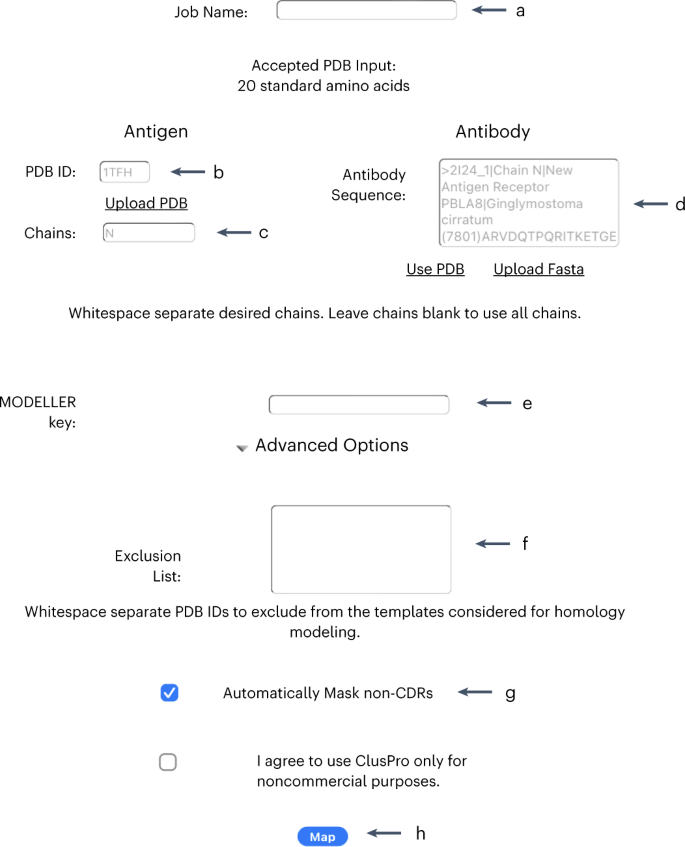
a, The space to enter the job name. b, The four-character code that specifies the PDB is entered here. c, The chains to be investigated go here. d, The FASTA code for the antibody is entered in this textbox. e, The user’s MODELLER key is entered here. f, The PDB IDs to be excluded in forming the homology model go here. g, Click here to select/deselect masking non-CDR regions. h, Submit the job by clicking ‘Map’.
-
4
(Optional) Enter a job name for the submission.
Critical step
If this option is left blank, a unique name will be provided by the server.
-
5
Input the antigen structure in PDB format. The docking procedure will remove all HETATM atoms from the PDB input, including water molecules, cofactors and ligands. Only the 20 standard amino acids and nucleotides will be retained.
-
6
Enter the structure. This can be done either by using a PDB ID or by uploading a PDB format file. If you import the antigen structure by using PDB ID, the four-character ID is used to automatically download the coordinates from https://www.rcsb.org. To upload the antigen structure by using a PDB format file, click on ‘browse’ and select the file to be uploaded.
Critical step
If there are multiple structures in the given PDB file, then our procedure will consider only the first structure.
Critical step
Nonstandard amino acid residues present in the PDB file are not supported and will result in an error when submitting.
-
7
In the ‘chains’ field, enter the chains on the antigen to be used for epitope mapping. The chain IDs should be separated by white space.
Critical step
If no chains are specified in this field, all the chains will be used.
-
8
Enter the antibody input type by using either of the available formats: as a sequence in FASTA format or as a structure in PDB format. The choice of the input format will determine which submission options will be visible and active for users on the webpage. As a result, the following steps for submission are broken into a sequence-based (FASTA format) procedure (A) and a structure-based (PDB format) procedure (B). Once the format type is selected, the user will follow the corresponding steps for that procedure.
-
(A)
FASTA format sequence-based procedure
-
(i)
Select the FASTA input type.
-
(ii)
Once the decision to use the FASTA format is made, there are two options for entering the sequence, as follows:
-
Enter the antibody sequence in FASTA format into the provided text box. An example is provided in the box.
-
Upload the antibody sequence as a FASTA file by using the upload FASTA option.
Critical step
The sequence in FASTA format should include the chain IDs.
-
-
(iii)
Enter a MODELLER key into the provided box. A MODELLER key (a passcode that allows users to continue with modeling the antibody) can be obtained from https://salilab.org/modeller/registration.html.
Critical step
A MODELLER key is a passcode obtained by users after registering on the above website. It allows users to use MODELLER, which is a crucial tool used in the antibody-modeling step. The key is not specific to the antibody but rather to the user.
Critical step
No sequence-based epitope prediction can be performed if the user does not have a MODELLER key.
-
(iv)
Select either of the two following advanced options available when using FASTA format as the input:
-
Define an exclusion list. If there are structures that should not be used by MODELLER as templates for the construction of the antibody structure, they should be listed. The models should be listed by PDB IDs separated by whitespace. This is beneficial for testing the server and/or comparing predictions based on different homolog availability.
-
Automatically mask non-CDRs. If selected, the server masks regions on the antibody that are not part of the CDRs. All areas of the antibody are considered if this option is not selected. This reduces the areas under consideration for docking and increases accuracy while reducing computational time.
Critical step
Selecting either advanced option is optional.
Critical step
By default, the masking option is already selected for users because it was found to yield the best results.
-
-
(i)
-
(B)
PDB format structure-based procedure
-
(i)
Select the PDB input type (as shown in Fig. 6). This option takes in the antibody structure in PDB format. The docking procedure will remove all HETATM atoms from the PDB input, including water, cofactors and ligands; only the 20 standard amino acids and nucleotides will be retained. If there are multiple models in the given PDB, the docking procedure will consider only the first.
Fig. 6: AbeMap job submit page after selecting the ‘Use PDB’ option for the antibody. 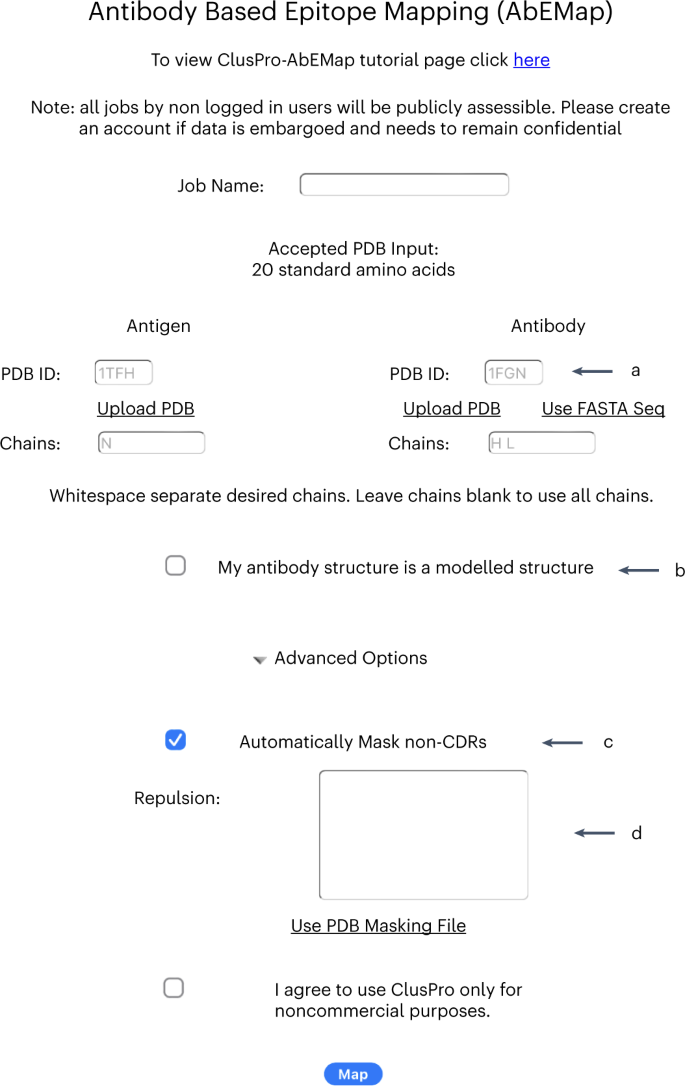
a, The four-character code that specifies the antibody PDB is entered here. b, If the structure is homology-based, select this checkbox. c, The option to automatically mask non-CDR regions is toggled here. d, The residues for repulsion are entered here.
-
(ii)
The structure can be entered in either of the two following ways:
-
Import the structure by using the corresponding four-character PDB ID that AbEMap uses to download the coordinates directly from https://www.rcsb.org.
-
Upload the PDB by clicking on ‘browse’ and selecting the PDB file to be uploaded.
Critical step
If there are multiple structures in the given PDB file, then our procedure will consider only the first structure.
Critical step
Nonstandard amino acid residues (labeled as ‘ATOM’ in the PDB file) are not supported and will result in an error when submitting. Entering the PDB ID does not cause an error.
-
-
(i)
-
(A)
-
9
In the ‘chains’ field, enter the chains on the antibody to be used for epitope mapping. The chain IDs should be separated by white space. If no chains are specified in this field, all the chains will be used.
-
10
Select if the antibody structure is a homology model. If the custom structure provided is a homology-modeled antibody, then select the option ‘My antibody structure is a modeled structure’.
Critical step
AbEMap provides a different set of weights and energy functions for model structures.
-
11
When using the PDB input options, two optional advanced options are currently present to select: to automatically mask non-CDRs (A) and to define repulsion (B).
-
(A)
Automatically mask non-CDRs
-
(i)
Select ‘automatically mask non-CDRs’ to have the server mask regions on the antibody that are not part of the CDRs. All areas of the antibody are considered if this option is not selected.
Critical step
By default, the masking option is already selected for users because it was found46 to yield the best results.
-
(i)
-
(B)
Define repulsion
-
(i)
As an alternative to automatic masking, you may want to manually provide information about what antibody residues are not in the binding interface. To bias the docking against those residues being in the binding interface, you can add a repulsion term to the residues you select. This can be achieved by providing a list of residues or a masking file and can be done in either of the following two ways:
-
Enter a list of residues in the ‘Repulsion’ text box. The residues should be separated by white space and have the form chain-residue number (e.g., a-27).
-
Generate a masking file by opening up the PDB file in PyMOL and using the sequence option to select the residues that should be excluded. Save this selection to a masking file in PDB format and upload.
-
-
(i)
-
(A)


Submitting the job and obtaining the results
Timing ~45–90 min
-
12
Once all the desired options have been selected, submit the job by using the ‘map’ button. Monitor the job status by using the ‘Queue’ page (Fig. 7; see Box 1 to interpret the status updates).
Fig. 7: AbEMap status page. 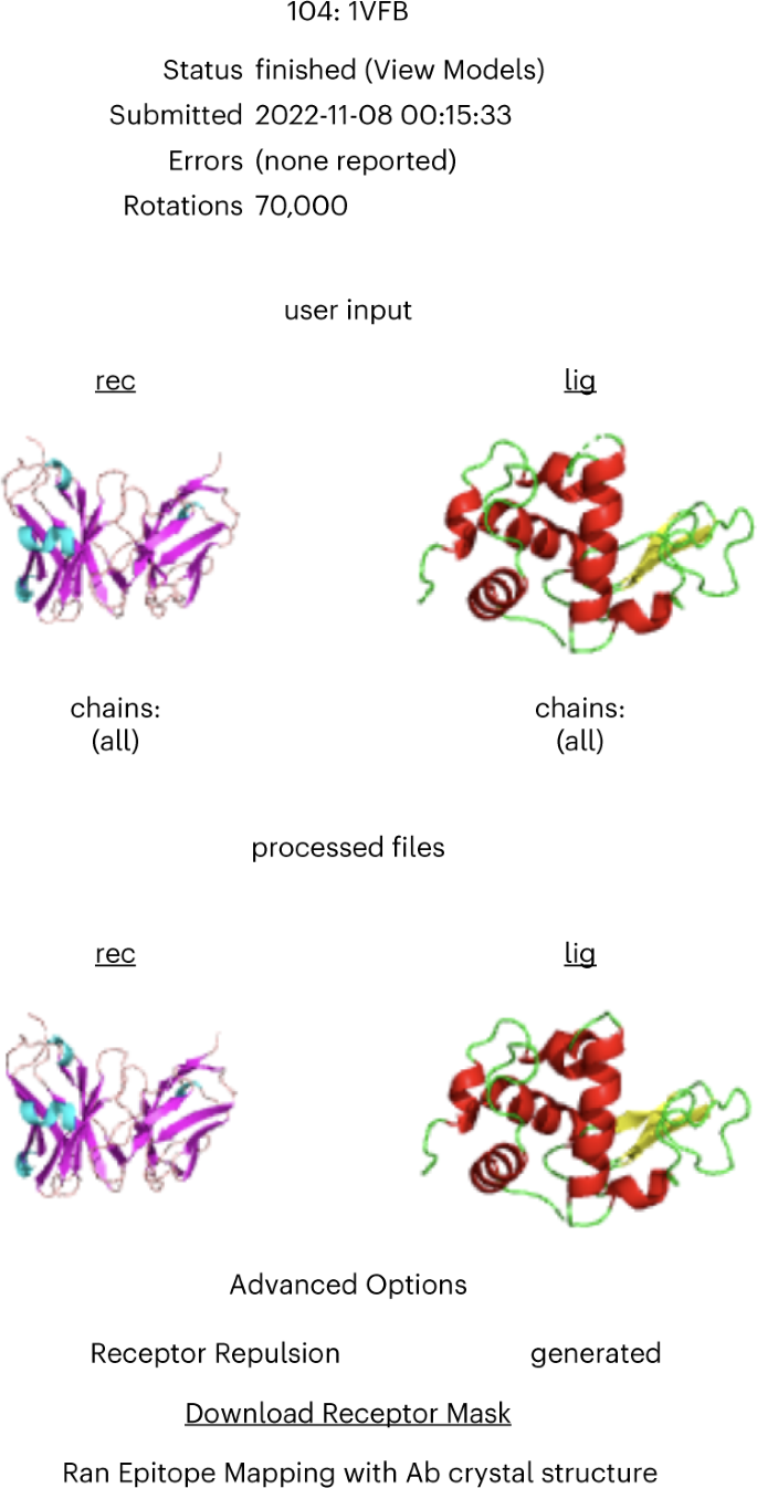
The page shows the job number in the AbeMap queue, the job ID, the status of the job, the submission date and time, potential errors and the number of rotations used during the docking stage. Further details on the job can be viewed by clicking the job number. Next, the page shows the input structures read by the program as cartoons and the structures after pre-processing. Finally, the advanced options selected by the user are shown at the bottom of the page.
Critical step
If the job has been submitted by using an account, an email will be sent on completion to notify the user that the job is done (Fig. 8).
-
13
Obtain the results for the job under the ‘Results’ tab.
Fig. 8: AbeMap job results page. 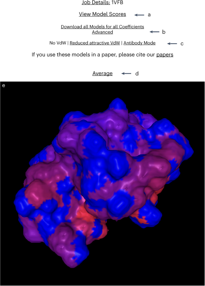
a, To view the results scores for the selected model, click here (Fig. 9). We recall that when using the homology-modeling option, AbeMap generates multiple models, one for each template. b, To view all the models for the job, select the ‘Advanced’ option. c, To view models obtained by using different coefficient sets, select the coefficients one wishes to view (No VdW; set 003; Reduced attractive VdW; set 005; Antibody Mode; set 007). d, To download the average PDB file with the likelihood scores in place of thermal factors, click here. e, The figure shows the PyMol-generated structure of the antigen in surface view. Blue to red shows increasing predicted likelihood scores.
Critical step
The results will remain on the server for ≥2 months, but after this time, they may be removed.


Analyzing the results
Timing ~30–40 min
-
14
View the results by selecting the ‘Results’ tab and selecting the job ID number. The results will differ depending on the input selection, FASTA (A) or PDB (B) format.
Critical
AbEMap produces several types of results files depending on the input format selected by the user. These files come in three formats: PDB, PSE and Residue Scoring files. Downloading and viewing the results are described in Box 3. The significance of these files and the means to access the information is provided in Box 4 (see also Table 2). Our AbEMap jobs result page is shown in Figs. 8 and 9.
Table 2 Energy function coefficient sets Fig. 9: AbeMap job results scores page. 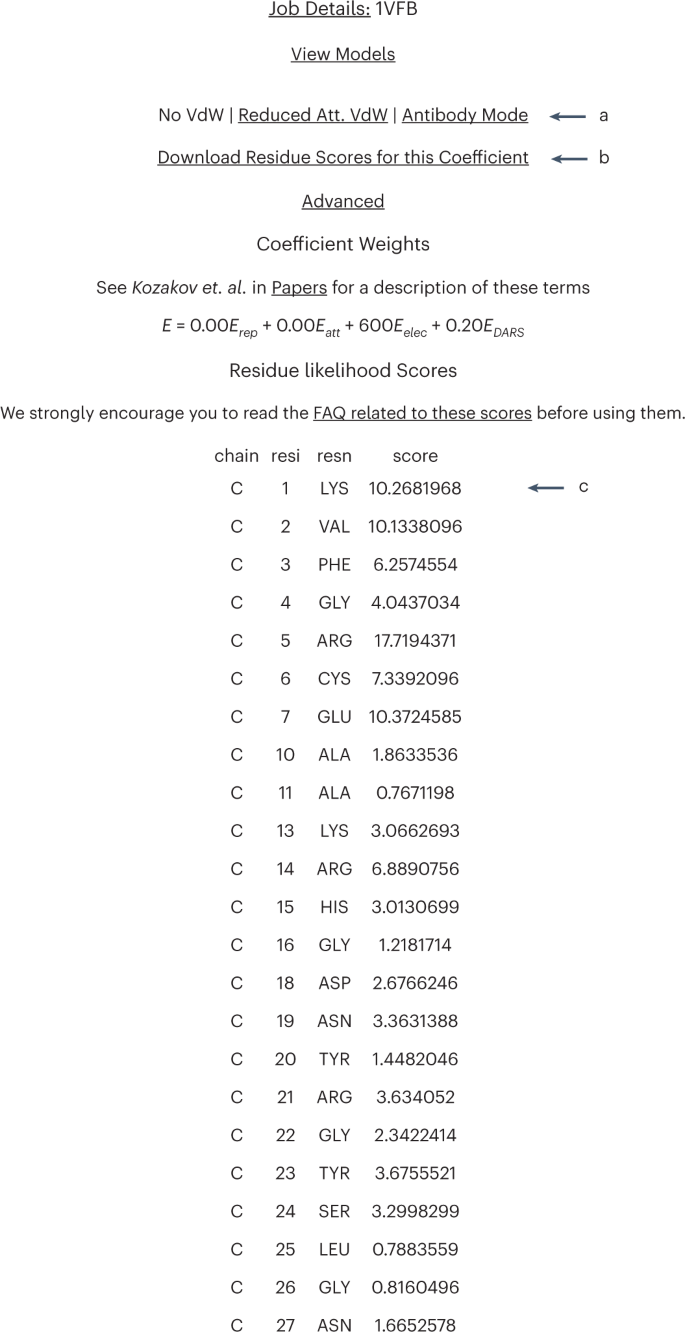
a, To view scores for different coefficient sets, select the coefficients to be viewed here. b, To download the scores for the selected coefficient, click here. c, The likelihood scores for each amino acid residue in the model are presented here. We recall that for epitope prediction, AbeMap uses 1,000 structures to calculate the frequency of each antigen surface atom’s occurrence in the antibody–antigen interface and defines the atomic epitope likelihood score as the Boltzmann weighted atomic interface occurrence frequency averaged over the ensemble of antibody structures. The residue likelihood scores are obtained by summing the atomic contributions for each residue.

Troubleshooting
Troubleshooting advice can be found in Table 3.
Timing
-
Steps 1–11, entering the basis inputs: ~1–2 min
-
Steps 12 and 13, submitting the job and obtaining the results: ~45–90 min
-
Step 14, analyzing the results: ~30–40 min
Anticipated results
Mapping hen egg white lysozyme epitopes binding two different antibodies
We mapped epitope residues of hen egg white (HEW) lysozyme with two different antigen receptors: shark single-domain antigen receptor 2I24 in the complex 2I25 and the D1.3 anti-HEW antibody fragment 1VFA in the complex 1VFB (see Supplementary Table 1). First, we consider that the antibodies are given by their X-ray structures. For the complex 2I25, the average mapping results of the HEW lysozyme (PDB ID 3LZT) in surface format (blue to red showing increasing likelihood score by AbEMap) are compared in Fig. 10a with the true orientation of the antigen receptor (PDB ID 2I24), shown as an orange cartoon. For comparison, the true placement and orientation of the D1.3 antibody (PDB ID 1FVA) in the other complex, 1VFB, on the same HEW antigen are shown as a semi-transparent green cartoon. To show the results for the 1VFB complex, the average mapping results of the HEW lysozyme (PDB ID 8LYZ) in surface format (blue to red showing increasing likelihood score by AbEMap) were obtained, with the green cartoon representing the D1.3 antibody (PDB ID 1FVA) and the antigen receptor (PDB ID 2I24) shown as a semi-transparent orange cartoon (Fig. 10b). In the top 20 predicted residues, using the coefficient set 007 (the no vdW option), AbEMap finds 10 of the true 22 residues for 3LZT and 11 of the true 19 epitope residues for 8LYZ (Supplementary Table 1).

a–f, All figures show the HEW lysozyme in surface view. Blue to red shows increasing predicted likelihood scores. The orange cartoons show the shark single-domain antigen receptor (PDB ID 2I24) in the complex 2I25, and the green cartoons show the D1.3 anti-HEW lysozyme antibody (PDB ID 1VFA) in the complex 1VFB. Whenever the cartoon is semi-transparent, the epitope-mapping result on the HEW lysozyme is shown for the other antibody. Panels a,c and e show, respectively, mapping results for the 2I24 antibody on 3LZT when the antibody 2I24 is defined by its X-ray structure, its AlphaFold2-generated model and just its sequence. Panels b,d and f show, respectively, mapping results for the 1VFA antibody on 8LYZ when the antibody 1VFA is defined by its X-ray structure, its AlphaFold2-generated model and just its sequence. As shown, the results for the two complexes are similar when using the independently solved X-ray structures. In the 20 top-ranked residues, AbeMap finds ~50% of the true epitope residues in both cases. When using the Alphafold2 models, the results get slightly better for 2I25 but slightly worse for 1VFB. However, the predictions are poor for both complexes when using the internal homology modeling of AbeMap, because most predicted antibody residues are in a region of the lysozyme on the opposite side from true antibody binding.
We used the same two antigen receptor complex examples (2I25 and 1VFB) with the HEW lysozyme as the antigen to demonstrate the modeled antibody structure mode of epitope mapping with AbEMap. The results of epitope mapping using the AlphaFold2-generated models of antibodies 1VFA and 2I24, respectively, were obtained, and the antigen is viewed from the same angle as with using X-ray structures as the input above, for easy comparison (Fig. 10c,d). In the top 20 predicted residues, mapping with AlphaFold2 models finds 11 of the true 22 residues on 3LZT and 7 of the 19 true epitope residues on 8LYZ, which is slightly less for 8LYZ but actually slightly more for 3LZT than the number found based on the X-ray structures of the antibodies using coefficient set 007 (the no vdW option). For coefficient set 003 (the reduced attractive VdW option), the results change to 8 of the 22 and 10 of the 19, respectively, thus better compared to using X-ray structures of 8LYZ but worse compared to using X-ray structures for 3LZT. The results when we have only the sequence of the antibody to start with, submitting the FASTA sequences of 1VFA and 2I24 (while excluding the crystal structures of the antibodies and their complexes 1VFB and 2I25, respectively, from the possible homologs for modeling the antibodies) are shown in Fig. 10e,f. We note that for 1VFA, AbEMap found 7 templates that pass the criteria described earlier (i.e., sequence identity above 20% and e-value below 1 × 10−40). Thus, eight different models—one for each template and one for the average model—were generated for each coefficient set. Nevertheless, in these cases, the homology models were not accurate enough for AbEMap to perform well, and only two and five true epitope residues, respectively, are captured in the top 20 predicted residues for 2I25 and 1VFB.
Examples of successful mapping using homology models of antibodies
As shown above, starting from the sequences of 1VFA and 2I24 and using the internal homology-modeling tool, AbEMap identified only a few epitope residues. However, the poor performance is an exception rather than the rule, and in most cases the accuracy of epitope prediction based on homology modeling is almost the same as that based on a separately crystallized X-ray structure of the antibody (Supplementary Table 1). Here, we show results for two complexes. 2W9E includes the structure of ICSM 18, the Fab fragment of a therapeutic antibody complexed with the fragment 119–231 of a human prion protein70. X-ray structures are available both for the antigen (PDB ID 1QM1) and the separately solved antibody (PDB ID 2W9D); see Supplementary Table 1. The second complex, 3MXW, includes the crystal structure of sonic hedgehog bound to the 5E1 fab fragment71. In this case, we also have the X-ray structures both for the antigen (3M1N) and the separately solved antibody (3MXV).
For the complex 2W9E, the average mapping results of the human prion protein (PDB ID 1QM1) in surface format (blue to red showing increasing likelihood score by AbEMap) are compared in Fig. 11a, with the true orientation of the antibody (PDB ID 2W9D) shown as an orange cartoon. Average mapping results of the sonic hedgehog (PDB ID 3M1N) in surface format (again, blue to red showing increasing likelihood score by AbEMap) were obtained, with the orange cartoon representing the antibody (PDB ID 3MXV) (Fig. 11b). In the top 20 predicted residues, when using the coefficient set 007 (the no vdW option), AbEMap found 10 of the true 19 epitope residues for 2W9E and 14 of the true 24 epitope residues for 3MXW (Supplementary Table 1). The results of epitope mapping using the AlphaFold2-generated models of antibodies 2W9D and 3MXV, respectively, are shown in Fig. 11c,d. In the top 20 predicted residues, mapping with AlphaFold2 models without templates found 13 epitope residues on 1QM1, thus almost the same as with the X-ray structure of the antibody, but only 4 epitope residues on 3M1N, representing a major drop in prediction accuracy. By using antibody templates in AlphaFold2, the results became even slightly worse, with only 12 and 3 epitope residues, respectively, identified. Results of mapping based only on the FASTA sequences of 2W9D and 3MXV, excluding the true complexes 2W9E and 3MXW, respectively, are shown in Fig. 11e,f. Using internal homology models in the top 20 predicted residues and the coefficient set 007 (the no vdW option), AbEMap found 14 of the true 19 residues for 2W9E and 9 of the true 24 epitope residues for 3MXW (Supplementary Table 1). Thus, the results were better than the ones obtained by using the antibody X-ray structure for 2W9E but worse for 3MXW (10 and 14 correct residue predictions, respectively). However, in both cases, the results were better than the ones obtained by using the Alphafold2 models (13 and 4 correct residues, respectively).

a–f, The first complex is a Fab fragment of a therapeutic antibody binding a fragment of a human prion protein. The second complex includes the crystal structure of sonic hedgehog bound to a fab fragment. As for the lysozyme-antibody complexes shown in Fig. 10, using the X-ray structures, AbeMap finds ~50% of true epitope residues in the 20 top-ranked residues (panels a and b). Using the AlphaFold2-generated models of antibodies, AbeMap finds almost the same residues for 2W9E as with the X-ray structure of the antibody but only four epitope residues for 3MXW, in this latter case representing a major drop in prediction accuracy (panels c and d, respectively). When using internal homology models and considering the 20 top-ranked residues, the results are better than with the antibody X-ray structure for 2W9E but worse for 3MXW (panels e and f). However, the differences are moderate, emphasizing that the use of homology models may provide prediction accuracy similar to that when X-ray structures are used.
Summary of the various AbEMap applications supported by source data
The most complex application of AbEMap is to map the epitopes on a given antigen crystal structure if only the sequence of the antibody is known and is entered by the user. We provide the results for such applications to the 40 antigens from the widely accepted protein–protein docking BM552. In the resulting PDB files, the thermal factors were changed to our protocol’s score to reflect the likelihood of each atom being in the epitope when in complex with the respective antibody (see https://doi.org/10.6084/m9.figshare.19652130.v2). The results also include the residue-based summary confusion matrix. The text file contains the TP, FP, false negative and true negative counts for each antibody–antigen complex at different residue-ranking thresholds (Top1, Top5, Top10,… Top120). This confusion matrix was used to generate Fig. 1l.
The simplest application of AbEMap is using X-ray crystal structures for both an antigen and an antibody (bound or unbound). We also provide the results of this type of application to the files of the 40 antigens and corresponding antibodies in the BM5 set52, with the thermal factors changed to our protocol’s score (see https://doi.org/10.6084/m9.figshare.19651314.v4). As in the previous paragraph, the text file contains the summary confusion matrix, which was used to generate Fig. 2.
AbEMap was also applied to the 23 antibody–antigen complexes that were more recently added to the docking benchmark set (BM5.5)29. However, AbEMap was unable to provide antibody models for two of the complexes, and hence we present results for the remaining 21 targets (see https://doi.org/10.6084/m9.figshare.19651428.v4). The thermal factors were again changed to our protocol’s score and are given by using the antigen crystal structure and either (i) the antibody crystal structure or (ii) only the antibody sequence. We also provide the confusion matrix, which was used to generate Fig. 4.
Finally, we present AbEMap results using the antigen X-ray structures in the BM5 set and antibody models predicted by the Alphafold2 program40, both with and without templates (see https://doi.org/10.6084/m9.figshare.21546897.v1). This data set refers to the summary results shown in Table 1. The results include (i) the top AlphaFold2-predicted antibody models using the program with templates or (ii) the top AlphaFold2-predicted antibody models obtained without templates. We add the corresponding pdb files of the AbEMap’s results for (iii) using the AlphaFold2 antibody models obtained with templates and (iv) using the AlphaFold2 antibody models obtained without templates. As in the other applications, the thermal factors were changed to our protocol’s score to reflect the likelihood of each atom being in the epitope when in complex with the respective antibodies. The confusion matrices are shown for the AbEMap results using the AlphaFold2 models (v) with templates and (vi) without templates.
Reporting summary
Further information on research design is available in the Nature Portfolio Reporting Summary linked to this article.
Data availability
Data for all cases tested in the benchmark set used can be found in the following figshare link: https://doi.org/10.6084/m9.figshare.c.6295842.v1. Detailed results and direct links for the server results are shown in Anticipated results.
Code availability
AbeMap is available as a server at https://abemap.cluspro.org/ free of charge for non-commercial applications. The server can be used without registration, but in that case, the results will be publicly accessible. The advantage of registering is that the job does not show up on the website, but this option is available only to users with educational or governmental email addresses. The server provides options to view the results online, but protein visualization tools allow for more convenient analyses. We use and recommend PyMOL, which was used to demonstrate the analysis of results in this protocol.
References
Montgomery, R. A., Cozzi, E., West, L. J. & Warren, D. S. Humoral immunity and antibody-mediated rejection in solid organ transplantation. Semin. Immunol. 23, 224–234 (2011).
Sela-Culang, I., Kunik, V. & Ofran, Y. The structural basis of antibody-antigen recognition. Front. Immunol. 4, 302 (2013).
Danilov, S. M. et al. Fine epitope mapping of monoclonal antibody 5F1 reveals anticatalytic activity toward the N domain of human angiotensin-converting enzyme. Biochemistry 46, 9019–9031 (2007).
Sela-Culang, I. et al. Using a combined computational-experimental approach to predict antibody-specific B cell epitopes. Structure 22, 646–657 (2014).
Ehrhardt, S. A. et al. Polyclonal and convergent antibody response to Ebola virus vaccine rVSV-ZEBOV. Nat. Med. 25, 1589–1600 (2019).
Goldstein, L. D. et al. Massively parallel single-cell B-cell receptor sequencing enables rapid discovery of diverse antigen-reactive antibodies. Commun. Biol. 2, 304 (2019).
Horns, F., Dekker, C. L. & Quake, S. R. Memory B cell activation, broad anti-influenza antibodies, and bystander activation revealed by single-cell transcriptomics. Cell Rep. 30, 905–913.e6 (2020).
Kozlova, E. E. G. et al. Computational B-cell epitope identification and production of neutralizing murine antibodies against Atroxlysin-I. Sci. Rep. 8, 14904 (2018).
Hua, C. K. et al. Computationally-driven identification of antibody epitopes. Elife 6, e29023 (2017).
Qi, T. et al. SEPPA 2.0—more refined server to predict spatial epitope considering species of immune host and subcellular localization of protein antigen. Nucleic Acids Res. 42, W59–W63 (2014).
Sun, J. et al. SEPPA: a computational server for spatial epitope prediction of protein antigens. Nucleic Acids Res. 37, W612–W616 (2009).
Zhou, C. et al. SEPPA 3.0-enhanced spatial epitope prediction enabling glycoprotein antigens. Nucleic Acids Res. 47, W388–W394 (2019).
Sweredoski, M. J. & Baldi, P. PEPITO: improved discontinuous B-cell epitope prediction using multiple distance thresholds and half sphere exposure. Bioinformatics 24, 1459–1460 (2008).
Rubinstein, N. D., Mayrose, I., Martz, E. & Pupko, T. Epitopia: a web-server for predicting B-cell epitopes. BMC Bioinforma. 10, 287 (2009).
Kulkarni-Kale, U., Bhosle, S. & Kolaskar, A. S. CEP: a conformational epitope prediction server. Nucleic Acids Res. 33, W168–W171 (2005).
Hopp, T. P. & Woods, K. R. Prediction of protein antigenic determinants from amino acid sequences. Proc. Natl Acad. Sci. USA 78, 3824–3828 (1981).
Jespersen, M. C., Peters, B., Nielsen, M. & Marcatili, P. BepiPred-2.0: improving sequence-based B-cell epitope prediction using conformational epitopes. Nucleic Acids Res. 45, W24–W29 (2017).
Potocnakova, L., Bhide, M. & Pulzova, L. B. An introduction to B-cell epitope mapping and in silico epitope prediction. J. Immunol. Res. 2016, 6760830 (2016).
Holmes, M. A., Buss, T. N. & Foote, J. Conformational correction mechanisms aiding antigen recognition by a humanized antibody. J. Exp. Med. 187, 479–485 (1998).
Li, Y., Li, H., Smith-Gill, S. J. & Mariuzza, R. A. Three-dimensional structures of the free and antigen-bound Fab from monoclonal antilysozyme antibody HyHEL-63. Biochemistry 39, 6296–6309 (2000).
Stanfield, R. L., Dooley, H., Verdino, P., Flajnik, M. F. & Wilson, I. A. Maturation of shark single-domain (IgNAR) antibodies: evidence for induced-fit binding. J. Mol. Biol. 367, 358–372 (2007).
Braden, B. C. et al. Three-dimensional structures of the free and the antigen-complexed Fab from monoclonal anti-lysozyme antibody D44.1. J. Mol. Biol. 243, 767–781 (1994).
Halperin, I., Ma, B., Wolfson, H. & Nussinov, R. Principles of docking: an overview of search algorithms and a guide to scoring functions. Proteins 47, 409–443 (2002).
Comeau, S. R., Gatchell, D. W., Vajda, S. & Camacho, C. J. ClusPro: a fully automated algorithm for protein-protein docking. Nucleic Acids Res. 32, W96–W99 (2004).
Comeau, S. R., Gatchell, D. W., Vajda, S. & Camacho, C. J. ClusPro: an automated docking and discrimination method for the prediction of protein complexes. Bioinformatics 20, 45–50 (2004).
Kozakov, D. et al. The ClusPro web server for protein-protein docking. Nat. Protoc. 12, 255–278 (2017).
Kozakov, D., Brenke, R., Comeau, S. R. & Vajda, S. PIPER: an FFT-based protein docking program with pairwise potentials. Proteins 65, 392–406 (2006).
Brenke, R. et al. Application of asymmetric statistical potentials to antibody-protein docking. Bioinformatics 28, 2608–2614 (2012).
Guest, J. D. et al. An expanded benchmark for antibody-antigen docking and affinity prediction reveals insights into antibody recognition determinants. Structure 29, 606–621.e5 (2021).
Krawczyk, K., Liu, X., Baker, T., Shi, J. & Deane, C. M. Improving B-cell epitope prediction and its application to global antibody-antigen docking. Bioinformatics 30, 2288–2294 (2014).
Krawczyk, K., Baker, T., Shi, J. & Deane, C. M. Antibody i-Patch prediction of the antibody binding site improves rigid local antibody-antigen docking. Protein Eng. Des. Sel. 26, 621–629 (2013).
Sikora, M. et al. Computational epitope map of SARS-CoV-2 spike protein. PLoS Comput. Biol. 17, e1008790 (2021).
Marks, C. & Deane, C. M. How repertoire data are changing antibody science. J. Biol. Chem. 295, 9823–9837 (2020).
Vajda, S., Porter, K. A. & Kozakov, D. Progress toward improved understanding of antibody maturation. Curr. Opin. Struct. Biol. 67, 226–231 (2021).
Porter, K. A. et al. Template-based modeling by ClusPro in CASP13 and the potential for using co-evolutionary information in docking. Proteins 87, 1241–1248 (2019).
Padhorny, D. et al. Protein-protein docking by fast generalized Fourier transforms on 5D rotational manifolds. Proc. Natl Acad. Sci. USA 113, E4286–E4293 (2016).
Ngan, C. H. et al. FTSite: high accuracy detection of ligand binding sites on unbound protein structures. Bioinformatics 28, 286–287 (2012).
Desta, I. T. et al. Mapping of antibody epitopes based on docking and homology modeling. Proteins 91, 171–182 (2023).
Jumper, J. et al. Applying and improving AlphaFold at CASP14. Proteins 89, 1711–1721 (2021).
Jumper, J. et al. Highly accurate protein structure prediction with AlphaFold. Nature 596, 583–589 (2021).
Tunyasuvunakool, K. et al. Highly accurate protein structure prediction for the human proteome. Nature 596, 590–596 (2021).
Evans, R. et al. Protein complex prediction with AlphaFold-Multimer. Preprint at https://www.biorxiv.org/content/10.1101/2021.10.04.463034v2 (2021).
Ghani, U. et al. Improved docking of protein models by a combination of Alphafold2 and ClusPro. Preprint at https://www.biorxiv.org/content/10.1101/2021.09.07.459290v1 (2021).
Ko, J. & Lee, J. Can AlphaFold2 predict protein-peptide complex structures accurately? Preprint at https://www.biorxiv.org/content/10.1101/2021.07.27.453972v1.full (2021).
Mirdita, M., Ovchinnikov, S. & Steinegger, M. ColabFold: making protein folding accessible to all. Nat. Methods 19, 679–682 (2022).
Desta, I. T., Porter, K. A., Xia, B., Kozakov, D. & Vajda, S. Performance and its limits in rigid body protein-protein docking. Structure 28, 1071–1081.e3 (2020).
Webb, B. & Sali, A. Comparative protein structure modeling using MODELLER. Curr. Protoc. Prot. Sci. 86, 2.9.1–2.9.37 (2016).
Katchalski-Katzir, E. et al. Molecular surface recognition: determination of geometric fit between proteins and their ligands by correlation techniques. Proc. Natl Acad. Sci. USA 89, 2195–2199 (1992).
Lindemann, S. R., Yershova, A. & LaValle, S. M. Incremental grid sampling strategies in robotics. In Algorithmic Foundations of Robotics VI (eds Erdmann, M., Overmars, M., Hsu, D., & van der Stappen, F.) 313–328 (Springer Berlin, Heidelberg, 2005).
Chuang, G. Y., Kozakov, D., Brenke, R., Comeau, S. R. & Vajda, S. DARS (Decoys As the Reference State) potentials for protein-protein docking. Biophys. J. 95, 4217–4227 (2008).
Lee, B. & Richards, F. M. The interpretation of protein structures: estimation of static accessibility. J. Mol. Biol. 55, 379–400 (1971).
Vreven, T. et al. Updates to the integrated protein-protein interaction benchmarks: docking benchmark version 5 and affinity benchmark version 2. J. Mol. Biol. 427, 3031–3041 (2015).
Fox, N. K., Brenner, S. E. & Chandonia, J. M. SCOPe: structural classification of proteins—extended, integrating SCOP and ASTRAL data and classification of new structures. Nucleic Acids Res. 42, D304–D309 (2014).
Akbar, R. et al. A compact vocabulary of paratope-epitope interactions enables predictability of antibody-antigen binding. Cell Rep. 34, 108856 (2021).
Salamanca Viloria, J., Allega, M. F., Lambrughi, M. & Papaleo, E. An optimal distance cutoff for contact-based Protein Structure Networks using side-chain centers of mass. Sci. Rep. 7, 2838 (2017).
Stave, J. W. & Lindpaintner, K. Antibody and antigen contact residues define epitope and paratope size and structure. J. Immunol. 191, 1428–1435 (2013).
Pittala, S. & Bailey-Kellogg, C. Learning context-aware structural representations to predict antigen and antibody binding interfaces. Bioinformatics 36, 3996–4003 (2020).
Sivasubramanian, A., Sircar, A., Chaudhury, S. & Gray, J. J. Toward high-resolution homology modeling of antibody Fv regions and application to antibody-antigen docking. Proteins 74, 497–514 (2009).
Padhorny, D. et al. ClusPro in rounds 38 to 45 of CAPRI: toward combining template-based methods with free docking. Proteins 88, 1082–1090 (2020).
Weitzner, B. D. et al. Modeling and docking of antibody structures with Rosetta. Nat. Protoc. 12, 401–416 (2017).
Lepore, R., Olimpieri, P. P., Messih, M. A. & Tramontano, A. PIGSPro: prediction of immunoGlobulin structures v2. Nucleic Acids Res. 45, W17–W23 (2017).
Klausen, M. S., Anderson, M. V., Jespersen, M. C., Nielsen, M. & Marcatili, P. LYRA, a webserver for lymphocyte receptor structural modeling. Nucleic Acids Res. 43, W349–W355 (2015).
Schritt, D. et al. Repertoire Builder: high-throughput structural modeling of B and T cell receptors. Mol. Syst. Des. Eng. 4, 761–768 (2019).
Karami, Y. et al. DaReUS-Loop: a web server to model multiple loops in homology models. Nucleic Acids Res. 47, W423–W428 (2019).
Dunbar, J. et al. SAbPred: a structure-based antibody prediction server. Nucleic Acids Res. 44, W474–W478 (2016).
Marks, C. & Deane, C. M. Antibody H3 structure prediction. Comput. Struct. Biotechnol. J. 15, 222–231 (2017).
Lensink, M. F. et al. Blind prediction of homo- and hetero-protein complexes: the CASP13-CAPRI experiment. Proteins 87, 1200–1221 (2019).
Ruffolo, J. A., Guerra, C., Mahajan, S. P., Sulam, J. & Gray, J. J. Geometric potentials from deep learning improve prediction of CDR H3 loop structures. Bioinformatics 36, i268–i275 (2020).
Jespersen, M. C., Mahajan, S., Peters, B., Nielsen, M. & Marcatili, P. Antibody specific B-Cell epitope predictions: leveraging information from antibody-antigen protein complexes. Front. Immunol. 10, 298 (2019).
Antonyuk, S. V. et al. Crystal structure of human prion protein bound to a therapeutic antibody. Proc. Natl Acad. Sci. USA 106, 2554–2558 (2009).
Maun, H. R. et al. Hedgehog pathway antagonist 5E1 binds hedgehog at the pseudo-active site. J. Biol. Chem. 285, 26570–26580 (2010).
Acknowledgements
This investigation was supported by grants DBI 1759277 and AF 1645512 from the National Science Foundation and R35GM118078, R21GM127952 and RM1135136 from the National Institute of General Medical Sciences.
Author information
Authors and Affiliations
Contributions
I.T.D., S.K., D.K., D.B. and Y.K. developed the methodology. I.T.D., S.K. and G.J. developed the server. I.T.D., U.G., M.A. and D.B. performed the experiments. I.T.D., S.K. and S.V. prepared the manuscript. D.K. and D.M.S. reviewed the paper.
Corresponding authors
Ethics declarations
Competing interests
The PIPER docking program, on which the ClusPro AbEMap server is based, has been licensed by Boston University to Acpharis Inc. Acpharis, in turn, offers commercial sublicenses of PIPER. D.K. and S.V. consult for Acpharis and own stock in the company, and D.B. is the acting CEO of the company. However, both the ClusPro and AbEMap servers are free for non-commercial use.
Peer review
Peer review information
Nature Protocols thanks Pritam Kumar Panda, Mohammad Mostafa Pourseif and Bruno Villoutreix for their contribution to the peer review of this work.
Additional information
Publisher’s note Springer Nature remains neutral with regard to jurisdictional claims in published maps and institutional affiliations.
Related links
Key references using this protocol
Desta, I. T. et al. Proteins 91, 171–182 (2023): https://doi.org/10.1002/prot.26420
Porter, K. A. et al. Proteins 87, 1241–1248 (2019): https://doi.org/10.1002/prot.25808
Kozakov, D. et al. Nat. Protoc. 12, 255–278 (2017): https://doi.org/10.1038/nprot.2016.169
Padhorny, D. et al. Proc. Natl Acad. Sci. USA 113, E4286–E4293 (2016): https://doi.org/10.1073/pnas.1603929113
Ngan, C. H. et al. Bioinformatics 28, 286–287 (2012): https://doi.org/10.1093/bioinformatics/btr651
Key data used in this protocol
Desta, I. T. et al. Proteins 91, 171–182 (2023): https://doi.org/10.1002/prot.26420
Supplementary information
Supplementary Information
Supplementary Figs. 1 and 2 and Tables 1–3
Rights and permissions
Springer Nature or its licensor (e.g. a society or other partner) holds exclusive rights to this article under a publishing agreement with the author(s) or other rightsholder(s); author self-archiving of the accepted manuscript version of this article is solely governed by the terms of such publishing agreement and applicable law.
About this article

Cite this article
Desta, I.T., Kotelnikov, S., Jones, G. et al. The ClusPro AbEMap web server for the prediction of antibody epitopes. Nat Protoc 18, 1814–1840 (2023). https://doi.org/10.1038/s41596-023-00826-7
Received:
Accepted:
Published:
Issue Date:
DOI: https://doi.org/10.1038/s41596-023-00826-7
This article is cited by
-
InflANNet: a neural network predictor for Influenza A CTL and HTL epitopes to aid robust vaccine design
Bulletin of the National Research Centre (2023)
Comments
By submitting a comment you agree to abide by our Terms and Community Guidelines. If you find something abusive or that does not comply with our terms or guidelines please flag it as inappropriate.
