


« Prev Next »
Does it really matter whether a species has low or high levels of genetic variation? Biologists, conservationists, environmentalists, and informed citizens all worry about the impact of environmental change on the ecosphere. Although organisms cannot plan for environmental change, the more variation that exists in a population, the better prepared that population will be to adapt to change when it does occur. Note that the level of genetic variation within a population is dynamic: It reflects an ever-changing balance between processes, both random and nonrandom, which remove variation. Sometimes, the latter can overwhelm the former, leading to low levels of variation that cannot be reconstituted over ecological time scales. Researchers understand that variation arises through mutation and recombination, and they also know that natural selection can remove variation from a population. Moreover, scientists are well aware of the fact that real-life populations are not infinite, as the Hardy-Weinberg model requires us to assume. Together, these factors lead to a relentless loss of variation, a process referred to as genetic drift.
Genetic drift is the reason why we worry about African cheetahs and other species that exist in small populations. Drift is more pronounced in such populations, because smaller populations have less variation and, therefore, a lower ability to respond favorably — that is, adapt — to changing conditions. Thus, it's not just the number of cheetahs that worries us—it's also the decreased variation in those cheetahs.
Understanding the Mathematics of Drift
To get a feel for genetic drift, consider a population at Hardy-Weinberg equilibrium for a gene with two alleles, A and a. Let p = the relative frequency of the A allele, let q = the relative frequency of the a allele, and let p = q = 0.5. For no drift to occur, the frequencies of the alleles in successive generations must remain at 0.5. If N is the population size of diploid organisms, then the number of A alleles (denoted k) is equal to 2pN. Given this information, how can we calculate the exact probability that k remains equal to 2pN after a generation of random sampling? To do so, we begin with the general formula for the binomial distribution:
Pr(k | p, n) = [n! / k! (n - k)!]pk(1-p)n-k
The binomial distribution is used when (a) there are two possible outcomes of a trial, (b) the probability of each outcome remains the same across all trials, and (c) all trials are independent of each other. Here, the two possible outcomes (i.e., the allele sampled in a gamete) are A and a, the probability of sampling a gamete with the A allele is p, there are n = 2N trials (i.e., gametes sampled), and k of these trials result in the A allele. The term [n! / (k! (n -k)!)] gives the number of ways that one can observe exactly k "successes" (defined here as A alleles) and n -k "failures" (defined here as a alleles). The term pk (1-p)n - k is the exact probability of observing any given order of k "successes" and n - k "failures." Therefore, the product of these terms gives the exact probability of observing k "successes" and n - k "failures," given that one is unconcerned about their order.
Using the formula for the binomial distribution, we can calculate the exact probability that k = 2pN for a range of N. Doing so yields the following results:
| Population size (N) | 2 | 5 | 10 | 50 | 100 | 500 | 1,000 | 10,000 |
| Gene Copies (2N) | 4 | 10 | 20 | 100 | 200 | 1,000 | 2,000 | 20,000 |
| Pr(k | p, n = 2N) | .375 | .246 | .176 | .080 | .056 | .025 | .018 | .006 |
At first glance, these results might seem backward. According to the table, the probability that the allele frequencies will remain unchanged is higher for the smaller populations! However, that's only part of the story. In all of these cases, it's more likely that the allele frequencies will change, and it is actually the magnitude of the change that matters. To see what this means, let's focus on those populations where N = 5, N = 50, and N = 500. Figures 1 through 3 show the probabilities of allele frequencies in the next generation of each of these populations.
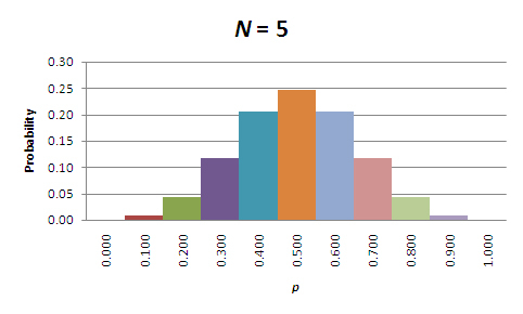
Figure 1: Probabilities of allele frequencies in the next generation, in a population of five organisms (N=5).
© 2008 Nature Education All rights reserved. 
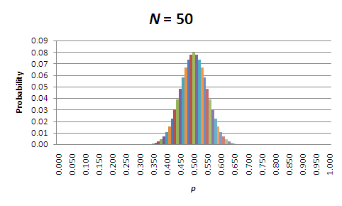
Figure 2: Probabilities of allele frequencies in the next generation, in a population of 50 organisms (N=50).
© 2008 Nature Education All rights reserved.
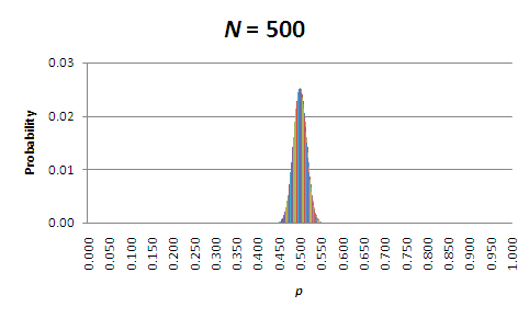
Figure 3: Probabilities of allele frequencies in the next generation, in a population of 500 organisms (N=500).
© 2008 Nature Education All rights reserved.
When looking at these figures, it should be evident that the breadth of the distribution narrows as population size increases. This is due to a decrease in sampling error. So, while allele frequencies are almost certain to change in each generation, the amount of change due to sampling error decreases as the population size increases. Perhaps the most important point is that the direction of the change is unpredictable; allele frequencies will randomly increase and decrease over time. Furthermore, when change does occur, sampling to produce the next generation will center on the new value of p. Thus, given enough time, in the absence of factors that maintain both alleles (e.g., balancing selection), p will drift to either 0.0 or 1.0; in other words, one allele will drift to fixation, and the other will drift to extinction. The time that it takes for this to occur depends on the starting frequencies of the alleles and, of course, the population size (see below under "The Population Genetic Consequences of Ne").
Effective Population Size
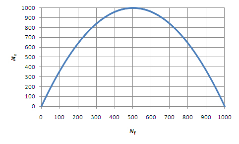
Figure 4: The relationship between Ne and Nf in a population of 1000 mating individuals.
© 2008 Nature Education All rights reserved.
- There are equal numbers of males and females, all of whom are able to reproduce.
- All individuals are equally likely to produce offspring, and the number of offspring that each produces varies no more than expected by chance.
- Mating is random.
- The number of breeding individuals is constant from one generation to the next.
Essentially, anything that increases the variance among individuals in reproductive success (above sampling variance) will reduce Ne (the size of an ideal population that experiences genetic drift at the rate of the population in question). For example, consider the effect of unequal numbers of mating males and females. In an ideal population, all males and all females would have an equal chance of mating. However, in situations in which one sex outnumbers the other, an individual's chance to mate is now affected by its sex, even if all individuals within each sex have an equal chance to mate. In this situation, effective population size can be predicted by the formula Ne = 4NmNf/(Nm + Nf), where Nm is the number of males and Nf is the number of females. Figure 4 shows the relationship between Ne and Nf in a population of 1,000 mating individuals. In an ideal population, all individuals have an equal opportunity to pass on their genes. In real life, however, this is rarely the case, and Ne is particularly sensitive to unequal numbers of males and females in the population.
The Population Genetic Consequences of Ne
One way to think about the relationship between Ne and genetic drift is to consider the time required for the fixation of one allele or the other if we assume selective neutrality. Motoo Kimura and Tomoka Ohta (1969) showed that this time—denoted E(T)—depends on two parameters, Ne and p. Specifically,
E(T) = -4Ne [p ln p + (1-p) ln (1-p)] generations
Therefore, fixation time scales with Ne. This time is maximized when p equals 0.5, and it falls off dramatically as one allele or the other becomes more rare at the generation we consider to be our starting point. Perhaps this is intuitive, but because intuition can sometimes be misleading, it's good that a formal mathematical treatment confirms our suspicions!
If we set p to 0.5, then one or the other allele should drift to fixation, on average, in 2.77 Ne generations. This would be 13,863 generations for a population with Ne equal to 5,000. However, if p is 0.25 (or 0.75), E(T) drops to 11,246 generations, and if p is 0.1 (or 0.9), E(T) drops considerably to only 6,502 generations. Moreover, if p is 0.01 (or 0.99), we can expect fixation to occur in just 1,120 generations.
Another way to think about drift is to consider the rate at which variation is lost. As in the previous example, this depends on Ne and the starting value of p. Here, we define "heterozygosity" (H) as the proportion of individuals who are heterozygous (2pq under Hardy-Weinberg assumptions). If H0 is the initial heterozygosity of the population, then the heterozygosity after t generations (Ht) can be calculated using the following equation:
Ht = (1-1/2Ne)tH0
According to this equation, H is expected to decline by a factor of 1/2Ne in each generation. Thus, the lower the effective population size, the faster heterozygosity will be lost.
Changing Population Size
Effective population size is also sensitive to changes in census population size over time. In a discrete generation model, Ne is calculated as the harmonic mean of the population sizes at each generation (i.e., the reciprocal of the mean of the reciprocals), as shown in the following equation:
Ne = [SNi-1/k]-1
In this equation, Ni is population size at generation i, and k is the number of generations. Note that the harmonic mean is always lower than the arithmetic mean (often considerably lower), and it is especially sensitive to the lowest values of Ni. This has special relevance to two related scenarios: a population bottleneck and a founder event. In the case of a population bottleneck, population size is substantially reduced for some period of time. In the case of a founder event, a small sample of a larger population becomes geographically isolated. In either case, the population size is dramatically reduced, at least temporarily. The effects of this reduction on genetic variation depend on both the size of the population during the reduction phase and the duration of the reduction phase.
Let's place this idea in context. Consider that, depending on the measure used, randomly chosen humans tend to differ at less than 1/1,000 of their DNA positions. Based on molecular population theory, the implication is that humans have an effective population size in the order of tens of thousands of individuals. However, we know that our census population size is currently well over 6 billion! Even though the human population has exploded, our standing genetic variation largely reflects a much smaller past population size. Remember, harmonic means are especially sensitive to the smallest values, so our Ne still mainly reflects the much lower past population size. In fact, it is almost certain to do so for as long as humans survive as a species. Barring the possibility of moving to another planet, the expected eventual destruction of Earth by the Sun does not allow enough time for us to recover a value of Ne close to our current census size.
This concept is relevant to conservation as well. A species that loses genetic variation to drift (e.g., because its census population has gone through a severe bottleneck) will have a very hard time recovering the lost variation, because Ne is most sensitive to the smallest population sizes over time. In fact, even if the census size of the population can be increased (perhaps through captive breeding efforts), the genetic variation may continue to decrease, because Ne still reflects the recent bottleneck.
References and Recommended Reading
Kimura, M. & Ohta, T. The average number of generations until fixation of a mutant gene in a population. Genetics 61, 763–771 (1969).