Modeling Sea Level Rise

Past climate changes in Earth's history have been accompanied by very large sea level changes. Just think of the Ice Ages that our planet has repeatedly gone through over the past two million years, as a result of slow, periodic changes in the Earth's axis of rotation and orbit around the sun. At the height of the last Ice Age, 20,000 years ago, global sea level was a full 120 meters lower than today, because so much of the ocean's water was locked up in the huge ice sheets covering large parts of the continents (IPCC 2007). Yet, global temperature was only about 4-7 ºC colder then (Schneider von Deimling et al. 2006).

Going back further in time, we find warmer climates. During the Pliocene, three million years ago, sea level was about 25-35 meters higher than today, while temperatures were just 2-3 ºC warmer (Dowsett and et al. 1994). And during the Eocene, 40 million years ago, the Earth was almost ice-free for the last time, due to elevated CO₂ levels related to plate tectonics. That meant that sea level was around 70 meters higher than today - that is also how much the ice on Earth today (mostly situated on Greenland and Antarctica) could raise sea level, should it all melt.

The Earth's history thus teaches us to expect large changes in sea level as we are warming up the climate with our emissions of greenhouse gases. But how much and how fast will sea level rise?

Physical models aim to describe quantitatively the different physical processes that contribute to sea level rise. Global sea level can be raised in three fundamentally different ways:

(i) By altering the volume of the existing ocean water mass by warming, a process called ‘thermal expansion'.

(ii) By adding water mass. Mass addition comes primarily from melting land ice, i.e. from mountain glaciers, small ice caps and the big ice sheets on Greenland and Antarctica. Melting sea ice hardly affects global sea level, since it already floats on the sea displacing water corresponding to its weight (Archimedes' principle). Mass addition (or removal) can to some extent also come from water stored on land in liquid form, e.g. from storage of water in human-built reservoirs, which corresponds to about 3 cm worth of sea level (Chao et al. 2008), or from pumping up water from deep aquifers for irrigation purposes which ends up in the ocean (Wada et al. 2010).

(iii) By changing the depths of the global ocean basins by movements of the Earth's crust. This is a very long-term process of lesser relevance on the century time scale, but it is currently estimated as causing a drop in sea level at a rate of 3 cm per century due to glacial isostatic adjustment (GIA), i.e. the ongoing adjustment process of the Earth's crust after the big ice sheets of the last Ice Age have disappeared.

We will discuss local sea level changes in a separate section below.

Of these key processes, thermal expansion can be modeled with 3-dimensional ocean circulation models, a standard component of coupled climate models. The crucial factor is how fast heat penetrates from the surface into the ocean, and where. The uncertainty comes, e.g., from the intensity of mixing of different ocean layers and from changes in ocean circulation. For a given emissions scenario, (IPCC 2007) estimates about a factor of two uncertainty in the thermal expansion; for moderate warming (A1B scenario) the best estimate is around 20 cm rise by 2100.

The melting of mountain glaciers is difficult to calculate from physical models because there is such a large number and variety of glaciers - the World Glacier Inventory contains ~123,000 glaciers (Radic and Hock 2010). It is impossible to model the dynamics of each glacier individually, so that semi-empirical scaling laws are used instead. Since satellite imagery reveals only the surface area, even the total volume of glacier ice is uncertain, with estimates ranging from 24 cm (Raper and Braithwaite 2005) to 60 cm (Radic and Hock 2010) sea level equivalent. Hence, the sea level contribution from glacier melt up to the year 2100 could be as little as 5 cm (Raper and Braithwaite 2006), around 10 cm (IPCC 2007), or more than 37 cm (Bahr et al. 2009) for moderate global warming.

Even more uncertain is the contribution of the two huge ice sheets on Greenland and Antarctica. Although they are modeled individually by ice sheet models, these do not yet properly capture the full flow dynamics, especially the small-scale, fast-flowing outlet glaciers that drain ice into the ocean. The part that is more easily modeled is the surface mass balance: the difference between snow accumulation and melting at the ice surface. For Antarctica this is expected to be positive as a result of warming, since snow fall increases more than melting. For Greenland this is moderately negative. Overall, the IPCC report (IPCC 2007) projected a sea level contribution from the ice sheets that is close to zero, due to Greenland losing some mass (roughly between 5 and 10 cm sea level equivalent) and Antarctica gaining a similar amount.

Semi-empirical models try to exploit the link between observed sea level rise and observed global temperature changes in the past in order to predict the future. Starting point is the simple physical idea that sea level rises faster as it gets warmer:

dH/dt = a (T(t) - T0), (Eq 1)

(Rahmstorf 2007) where H is sea level, T is global temperature and T0 is a baseline temperature at which sea level is stable. The central parameter is the "sea level sensitivity" a, which measures how much the rate of sea level rise accelerates for a unit change in global temperature. A similar approach is widely used in modeling the surface mass balance of ice sheets and glaciers: the warmer it gets, the faster the ice melts.

The empirical part then is to determine the unknown parameters a and T0 from observational data. Fig. 1 shows an empirical fit between a global sea level reconstruction (Church and White 2006) and the global temperature data of the NASA Goddard Institute for Space Studies (GISS), which illustrates that the time evolution of the rate of sea level rise matches the shape of the observed temperature increase.

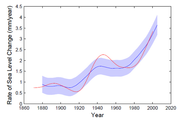
Figure 1: Rate of sea-level rise.

Rate of sea-level rise obtained from tide gauge observations (red line, smoothed with a filter half-width of 15 years) and computed from global mean temperature from Eq. 1 (dark blue line). The light blue band indicates the statistical error (one standard deviation) of the simple linear prediction. Note that the global temperature curve (blue) has a similar shape as the evolution of the rate of sea level rise.

© 2012 Nature Education Courtesy of Stefan Rahmstorf. All rights reserved.

Several refinements have been suggested for the semi-empirical method, like including a finite response time scale (Grinsted et al. 2009) and adding a second term for the short-term response of sea level (Vermeer and Rahmstorf 2009). It has been shown that a semi-empirical model also fits sea level proxy data for the past millennium: Medieval warmth explains a slow sea level rise from ~1000 to ~1400 AD at a rate of 0.6 mm/year. This is followed by a period of stable sea level from ~1400 to ~1900 AD, when anthropogenic warming leads to the rapid 20th Century rise (Kemp et al. 2011).

Semi-empirical models can be used to project future sea level rise from a scenario of future global temperature rise. This results in generally much higher projections than those of the IPCC, by a factor of two or even three (Rahmstorf 2010). For higher emissions scenarios, semi-empirical models typically predict more than one meter sea level rise by the year 2100. A comparison of IPCC and semi-empirical projections is shown in Fig. 2.

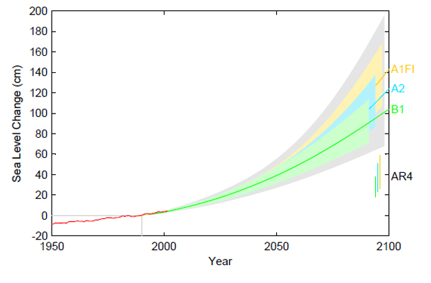
Figure 2: Projection of sea-level rise from 1990 to 2100.

Projection of sea-level rise from 1990 to 2100, based on IPCC temperature projections for three different emission scenarios (B1, A2 and A1FI). The sea-level range projected in the IPCC (IPCC 2007) for these scenarios is shown for
comparison in the bars on the bottom right. Also shown is the observations-based annual global sea-level data (Church and White 2006) (red) including artificial reservoir correction (Chao et al. 2008). The key difference between projections is that the IPCC projections would be realised if the rate of rise remains roughly constant at the 3.2 mm/year that is observed since satellite measurements of sea level began in 1993 (Church and White 2011), while the semi-empirical projections predict a future acceleration of sea level rise.

© 2012 Nature Education Reprinted with permission: IPCC, Church and White, Chao et al. All rights reserved.

An advantage of semi-empirical projections is that - by parameter fitting - they reproduce the observed past sea level rise. A fundamental limitation is that one cannot be sure that the simple empirical connection found for the past will continue to hold in future. Hence, they can only be a temporary tool until physical modeling has matured enough to provide more robust projections. Physical models also have the advantage of (in principle) allowing regional sea level projections.

To understand sea-level change at a particular coast, we must know the sum of global, regional and local trends related to changing ocean and land levels. Indeed, coastal managers are concerned about the interplay among global and local sea level rise, regional and local subsidence, and variations in sediment supply, as these determine the impacts at the coast and form the basis of management response plans.

Local sea level change can deviate from the global mean sea level change for a number of reasons.

- Ocean water moves around driven by winds and other factors, so that even if global water volume does not change (constant global-average sea level) there will be regional sea level changes. This can happen due to both natural oscillations in the climate system (such as El Niño / Southern Oscillation) and forced anthropogenic changes (e.g. a weakening of the Atlantic thermohaline circulation as found in most models in response to global warming (IPCC 2007)).

- The gravitational pull of land ice is reduced as the ice melts, which has a surprisingly large effect on the sea surface. For example, as ice on Greenland melts this will cause a global sea level rise, but a regional drop in sea level in a circular area around Greenland extending all the way to Fennoscandia (Mitrovica et al. 2001).

- There are vertical land movements that make the sea level change locally relative to the land - which is relevant for the impacts of sea level rise. This can have both natural reasons (i.e. tectonic processes as well as the still ongoing response to the massive ice loss at the end of the last ice age, called glacial isostatic adjustment), and anthropogenic reasons (like groundwater or oil extraction causing the coast to subside).

All these factors can in principle be modeled, but uncertainties are still large. Changes in ocean circulation are still difficult to predict. The problems in modeling ice melt were mentioned above in the context of global sea level - they are compounded by the fact that to compute the gravity effects, one also needs to know where the ice melts, not just the overall total. And while long-term local land motions (GIA) can be assumed to occur at a constant rate and thus extrapolated from past measurements, such measurements are not available everywhere, and local land motions can change due to recent effects (like local melting of glaciers, or changes in groundwater pumping).

Sea level change is a long-term response to climate change, due to the long characteristic time scales involved in heat penetrating into the ocean and in melting large amounts of ice. Hence the relatively small projected sea level rise by the year 2100, as compared to the changes measured in tens of meters that occurred in Earth's history (see Introduction). The rise by 2100 is only a small beginning of a much larger, multi-century response of ocean and ice sheets to elevated global temperatures.

For thermal expansion alone, IPCC has estimated a rise by between 60 and 200 cm over the next thousand years if global warming is stabilised between 2 and 4 ºC above present temperatures. However, the bulk of long-term sea level rise may be expected to come from ice melt.

Fig. 3 shows some estimates of possible sea level rise for the next 300 years. These should be treated as tentative given the uncertainties, but they indicate the likelihood of several meters of rise in the coming centuries. This would cause massive impacts along the world's coastlines.

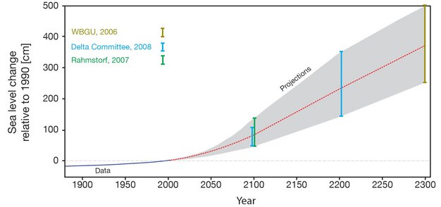
Figure 3: Sea level estimates out to the year 2300.

The light blue bars show the estimates for 2100 and 2200 by the Delta Commission (Vellinga et al. 2009), an expert panel appointed by the Dutch government. The olive bar for 2300 comes from the German Advisory Council on Global Change (WBGU - German Advisory Council on Global Change 2006). Both sources are expert assessments rather than model calculations. The green bar for 2100 comes from a semi-empirical model (Rahmstorf 2007).

© 2012 Nature Education Reprinted with permission: Vellinga et al., WBGU - German Advisory Council on Global Change, Rahmstorf All rights reserved.

The main impacts of sea level rise are increased coastal erosion and land loss (Fig. 4), increased risk of flooding during extreme events (storm surges) (Fig. 5), increasing groundwater levels up to 20-50 km inland, and salt water intrusion into freshwater resources. In addition, coral reefs and coastal ecosystems, like mangrove forests, turtle nesting beaches or coastal wetlands are threatened by sea level rise.

Figure 4: Coastal erosion on the Caribbean Island of Hispaniola.

© 2012 Nature Education Courtesy of Stefan Rahmstorf. All rights reserved.

Figure 5: Venice is suffering from increased frequency of flooding ("Acqua Alta") due to sea-level rise.

© 2012 Nature Education Courtesy of Stefan Rahmstorf. All rights reserved.

If sea level rise proceeds beyond one meter, coastal protection efforts (Fig. 6) will in many places not suffice and it is likely that some low-lying island states will have to be abandoned, such as the Maldives, Marshall Islands, Tuvalu, Kiribati and Tokelau, affecting half a million people. Many times more will be affected in large coastal cities. For New York, it has been estimated that a once-per-century storm surge event, which would cause major economic damage, must be expected once every three years if sea level were one meter higher (Rosenzweig and Solecki 2001).

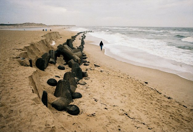
Figure 6: Coastal protection efforts on the German North Sea island of Sylt.

© 2012 Nature Education Courtesy of Stefan Rahmstorf. All rights reserved.