Abstract
The Texas power grid on the Gulf Coast of the United States is frequently hit by tropical cyclones (TCs) causing widespread power outages, a risk that is expected to substantially increase under global warming. Here we introduce a new approach that combines a probabilistic line failure model with a network model of the Texas grid to simulate the spatio-temporal co-evolution of wind-induced failures of high-voltage transmission lines and the resulting cascading power outages from seven major historical TCs. The approach allows reproducing observed supply failures. In addition, compared to existing static approaches, it provides a notable advantage in identifying critical lines whose failure can trigger large supply shortages. We show that hardening only 1% of total lines can reduce the likelihood of the most destructive type of outage by a factor of between 5 and 20. The proposed modelling approach could represent a so far missing tool for identifying effective options to strengthen power grids against future TC strikes, even under limited knowledge.
Main
Modern societies depend heavily on reliable access to electricity. Power outages have the potential to disrupt transportation and telecommunication networks, heating and health systems, the cooling chain underpinning food delivery and more1,2,3. Depending on the cause of power outages and the amount of physical damages to infrastructures, the recovery of the electric network and the social infrastructures dependent on it, often takes days or even months4. Such outages are often driven by extreme weather events. In Norway 90% of all overhead line failures are caused by extreme weather, which involves strong winds, icing and lightning strikes5. In February 2021, a winter storm in Texas led to outages that in turn caused a breakdown of the gas supply and thus the heating sector6,7,8. Further, tropical cyclone (TC) impacts can be particularly devastating. In the summer months, the Gulf Coast and the East Coast of the United States are frequently hit by TCs that entail widespread outages and costs of billions of dollars, as detailed in the State of Reliability reports of the North American Electric Reliability Corporation9,10. For example, Hurricane Ike hitting southeast Texas on 13 September 2008 destroyed around 100 towers of high-voltage transmission lines and cut off electric power for between 2.8 million and 4.5 million customers for weeks to months11,12. On 29 August 2021, Hurricane Ida made landfall in Louisiana and destroyed major transmission lines delivering power into New Orleans, causing power outages that affected more than a million customers13.
Reliability against line failures in high-voltage power grids is usually discussed in terms of the N-1 (rarely also N-2) security of the system, that is, the ability of the system to stay fully functional upon the failure of one or two elements14. When a line fails, the power flow automatically reroutes through the intact grid. To avoid damages from overloads caused by the rerouting, highly loaded lines are removed by automatic protection devices or, in some cases, manually from the network. These secondary failures of lines can trigger a cascade15,16,17,18,19,20,21 of additional failures. If N-1 security is given, single line failures do not trigger such cascades. However, multiple concurrent failures—as probably occurred in the US–Canadian blackout in 200322 and as are typical for TCs, which cause widespread primary damages—can trigger substantial secondary failures. These cascades play an important role in amplifying the resulting blackouts23.
The N-1 approach to system resilience cannot be scaled to such events. Even an exhaustive N-5 security assessment is infeasible, and major TCs often damage tens or even hundreds of lines. These damages cannot be fully mitigated by an electric network. N-1 security is typically studied by simulating the reaction of the system to every possible failure scenario. As the number of these scenarios scales exponentially with the number of failures, it is computationally infeasible to consider all possible scenarios for larger events.
Several earlier studies have analysed the spatial and temporal patterns of lines destroyed by TCs using statistical methods such as negative binomial regression models24,25 and non-stationary Poisson processes26. However, these studies did not consider the impact of these damages on the power grid. In an effort to address this gap, machine learning techniques were applied to predict power outages caused by various types of storm on a 2-km grid27, but this approach does not provide information on how these outages occur or how they can be prevented.
TC-induced failures affecting large numbers of lines have been recently studied from a detailed mechanistic perspective28,29,30,31. Aiming to capture the primary damages well, these works focus on the development of sophisticated line failure models. The TC impacts on the power grid are then described by removing all damaged elements at once or in large batches and using optimal dispatch models to estimate how much load such a damaged system can still provide. This requires the (rather strong) assumption of a perfect, omniscient system operator31,32,33. A further crucial limitation of this approach is that the optimization in these models ensures that operational bounds are never violated. Thus, these models do not capture failure cascades.
Here we go beyond the existing literature by introducing a co-evolution modelling approach. It combines a spatio-temporal stochastic line failure model with a stepwise modelling of the resulting power outages, accounting for automatic or manual line protection mechanisms and unavoidable overproduction. This approach allows us to (1) consider a large number of potential realizations of line failures along the TC’s tracks and (2) assess cascading secondary failures. Further, critical power lines in the high-voltage transmission system whose protection could most effectively prevent cascades and the associated widespread power outages can be identified. This is especially interesting from a climate change perspective because the proportion of very intense TCs in the North Atlantic is projected to increase under global warming34,35,36.
Modelling cascading losses in the Texas grid
Our co-evolution modelling approach explicitly captures the dynamical interplay of an extreme wind event with the power grid by temporally resolving both the primary wind damage and the resulting cascades of secondary failures. We will use this approach to study a selection of seven historical TCs that impacted the Texas power grid between 2003 and 2020. These cover different types of trajectory and intensity (Supplementary Note 1 and Supplementary Figs. 1 and 2). The selected storms include major hurricane-strength TCs, such as hurricanes Ike and Harvey that made landfall in Texas in September 2008 and August 2017, respectively, and destroyed numerous high-voltage (115–500 kV) transmission lines (about 106 (ref. 37) and 97 lines38 were reportedly destroyed by Harvey and Ike, respectively) (Fig. 1a). Further, we consider five TCs, that is, Hurricanes Claudette (2003), Hanna (2020) and Laura (2020) and Tropical Storms Erin (2007) and Hermine (2010) that caused less damage to the Texas grid39,40,41,42,43, either because they were substantially weaker (for example, Erin and Hermine) or because they primarily affected neighbouring states (for example, Hanna, which made landfall in Louisiana). The TCs considered here affected different parts of the Texas grid; Claudette, Erin and Hanna continued to move westward after landfall and affected the southern and western parts of the grid. The rest of the considered TCs were steered northward by the Coriolis effect after landfall and mainly affected the western parts of the grid34.
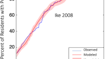
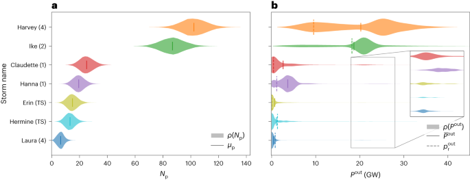
a, Probability distribution ρ of the total number of wind-induced line failures Np as generated by the probabilistic line failure model for each of the seven recent TCs hitting Texas. The storms are categorized according to the Saffir–Simpson scale (number in brackets behind the storms’ names), and tropical storms that did not reach hurricane strength at landfall are denoted by TS. TCs are sorted according to the means of the distributions μp, which are indicated as solid vertical lines. The mean numbers of damaged lines for Hurricane Harvey (105) and Hurricane Ike (90) are very close to the reported numbers in the high-voltage (115 kv to 500 kV) transmission grid (106 for Harvey and about 97 for Ike). b, Probability distribution of the associated total power outage Pout after TC passage. The dashed vertical lines prout indicate the reported power outages listed in Supplementary Table 1, and the solid vertical lines Pout represent the means. The inset highlights large cascading failures that can also occur for the less impactful TCs. Methods provides the model parameters used in the simulations. Each storm is presented with the same colour in a and b.
When a TC hits a power grid, lines do not collapse simultaneously but sequentially over the hours or days of the TC’s passage. Making use of the chronological order of the line destructions, we divide each considered TC landfall scenario into a sequence of 5-minute time steps. In most of these individual steps, only one additional line fails, that is, these situations can be addressed by power distribution models also used for N-1 or N-2 security assessments. At this resolution, it is also reasonable to assume that cascades of secondary failures have run their course before further lines are destroyed by the TC44,45 (further discussion regarding the temporal resolution is in Methods and Supplementary Note 9).
We solve individual scenarios by representing the Texas power grid in a direct current (d.c.) power flow approximation with conservative load balancing assumptions (Methods and Supplementary Notes 3 and 4). Our co-evolution approach allows us to account for the ‘path dependency’ of the solution: every time a line collapses, overload protection can cause more lines to fail. At the same time, control mechanisms are immediately activated to restore energy balance and limit the effect of the failures (Supplementary Note 4). If an islanded part of the grid cannot be rebalanced, this part and all lines in it are considered failed. Primary damages that occur later along the TC track then meet a partially destroyed, rebalanced grid. Thus, the effect of later failures can be more, or even less, intense. It is the resilience of these intermediate, partially destroyed states that ultimately decides whether the impact of the TC is amplified by secondary failures.
Unfortunately, neither detailed information about the topology of the exposed power grid, nor about the exact number and the location of power lines destroyed by the TCs, nor the type of consumers who lost power is publicly accessible. Here we use a synthetic model of the Texas power grid introduced by Birchfield et al., which includes four different high-voltage levels, 115, 161, 230 and 500 kV (ref. 46) (Methods and Supplementary Fig. 2).
The employed probabilistic line failure model is forced by the modelled historical wind fields of the studied TCs (Methods and Supplementary Note 2). The probability of line failure is described in terms of wind speeds and allows generating a large sample of temporally resolved realizations of line failure sequences, here 10,000 sequences per storm. These scenarios differ greatly with regard to the individual failed lines and thus cover a wide range of plausible scenarios (Fig. 1). In the default setting considered here, we assume a homogeneous base failure rate for all transmission lines. This is our main calibration parameter and is tuned to reproduce observed numbers of damaged lines and match power outages (Fig. 1a,b and Supplementary Note 5). By looking at five additional weaker storms, we found that our modelling results are aligned with the inclusive reports of power outages and rare damages in the transmission grid (Supplementary Note 5 and Supplementary Fig. 10).
The structure of outages
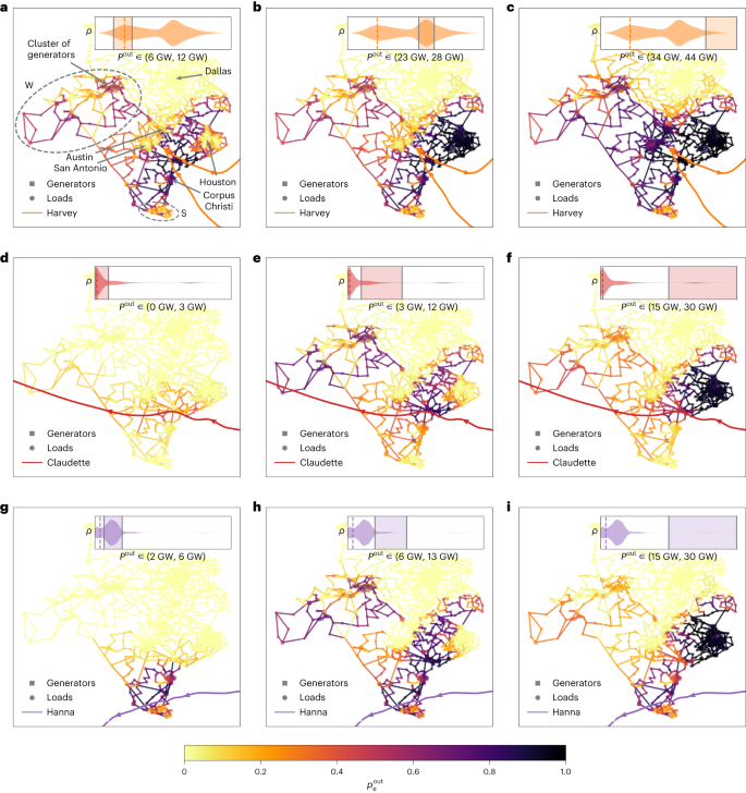
Caused by strong winds, primary damages are concentrated in areas close to the centre of the storm, and the number of primary line failures follows a Poisson binomial distribution. However, for all seven TCs, cascading secondary failures due to overload protection and unavoidable islanding substantially increase the total number of affected lines and can lead to large 20-GW to 30-GW power outages (Fig. 1b). As the most populous city in Texas and a major load centre, the disconnection of Houston from the electrical network causes the disconnection of a huge number of consumers. Many generators providing energy to the major load centres are clustered in the west of Texas. The largest events feature both of these regions going offline (Figs. 2d and 3, Supplementary Note 5 and Supplementary Fig. 9). Smaller events (Figs. 2c and 3a,d,g) tend to show damage patterns more localized to the storm tracks. The resulting distributions of total outages are heavily multimodal for all TCs (Fig. 1b).
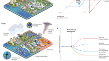
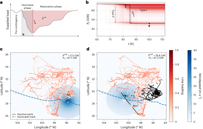
a, Schematic variation of power outage Pout and total energy not supplied Eout (red area) before (Pre-contingency), during (Hurricane phase) and after (Restoration phase) the TC passage (loosely based on ref. 38). b, Summary of all realizations of power outage trajectories simulated for Hurricane Claudette. Trajectories fall into two categories: those that aggregate damages gradually over time (Type I) and those that include a large cascade (Type II). c,d, States of the power grid at the beginning and the end of the TC passage for two exemplary Type I and Type II trajectories highlighted in panel b. Lines shown in black are destroyed (primary damages) or deactivated (secondary failures) during TC passage (Supplementary Video 1 shows the structure of failures during the simulation). The colour code of the remaining lines indicates relative line loading, with darker colours indicating higher relative loads. Blue dashed lines indicate the track of the storm centre and blue arrows denote the direction of the storm’s movement. Blue shaded circles indicate snapshots of the storm’s wind field, with darker colours indicating higher wind speeds. Methods and Supplementary Note 5 provide the specification of the model parameters and an animation of the cascading failures and load dynamics during the passage of Claudette.
a–i, Probability \({p}_\mathrm{e}\!^{\mathrm{out}}\) that the failure of a given power line is involved in three different modes of the power outage distribution for Harvey (a–c), Claudette (d–f) and Hanna (g–i). S represents the southern community and W the western region in Texas. Modes are indicated by the insets, and the exact ranges of considered power outages are shown below these insets. Probability \({p}_\mathrm{e}\!^{\mathrm{out}}\) is calculated as the number of realizations having a total outage within the specified ranges in which the considered line fails, divided by the total number of realizations in the specified range. The different elements of the Texas power grid are coloured according to their respective outage probability. The probability distributions shown in the insets are identical to those shown in Fig. 1b.
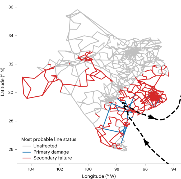
Large outages do not accumulate gradually over time. Instead the disconnections of the load centre of Houston and the production centre in the Northwest occur suddenly during one large cascade (Fig. 2b). Spatially, it is noteworthy that these cascading failures can lead to outages in areas not directly affected by the storm (Fig. 4 provides a comparison of the spatial distribution of primary damages and cascading, secondary failures caused by Hurricane Harvey). For instance, during Harvey, Hanna and Claudette, the northwestern section is not reached by strong winds (Fig. 3).
Transmission lines are coloured according to their most probable line status. Blue lines are most likely directly damaged by strong winds (primary damages), whereas red lines are most likely deactivated due to cascading secondary failures. Grey lines have a higher probability of remaining operational than failing due to primary damages or secondary failures (Supplementary Note 5 provides details on the model calibration).
To test the robustness of our results with regard to the details of the model calibration, we repeated the simulations for a wide range of failure rates and randomized the failure rates for each line (Supplementary Notes 5 and 6). Further, we used a large ensemble of 10,000 realizations for each storm to ensure that it represents a wide range of plausible grid states. We found the main characteristics of the cascading failure dynamics, such as the occurrence of sudden large cascades and multimodal outage distributions, to be robust (Supplementary Table 3). For instance, across all parameter settings, we find Harris County to be the most vulnerable part of the Texas grid to TC impacts, in line with a recent analysis of the National Centers for Environmental Information47. These findings suggest that our main results are independent of the details of the line failure model and its calibration.
Increasing resilience
We find that large cascades are triggered by the failure of individual lines. This suggests that hardening those lines that are likely to trigger cascades (for example, by replacing them with underground cables) could be an effective resilience-building strategy. To identify the critical lines that should be hardened, we define a priority index as the probability that the wind-induced damage of this specific line triggers a large cascade, that is, a cascade that increases the outage by more than 15 GW, averaged over all seven TCs (equations (2) and (4) in Methods). For most transmission lines, the priority index is zero, but 8% of them have a value above 10−4, and 20 lines (about 1% of the grid) have a priority index above 10−3.
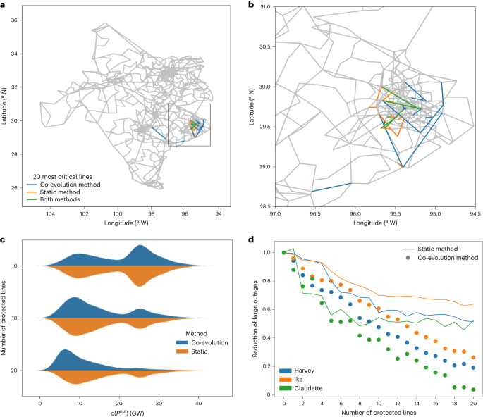
For comparison, we also calculate the priority index based on a conventional, static model in which all damages are applied at once. The static index of a line is then defined, analogously to the priority index, as the conditional probability of a large outage given that the line is in the set of lines damaged by a TC (Methods and Supplementary Note 7). According to both the co-evolution model and the static model, the critical lines are mostly located in and around Houston (Fig. 5a,b). However, the co-evolution model also identifies several critical lines not in the area that are not among those identified by the static model.
a, The 20 lines of the Texas power grid with the highest priority index (equation (4)) obtained from the static model (orange lines), the co-evolution model (blue lines) and both models (green lines). b, Detail enlargement (black rectangle in a) of Houston and Harris County, which contain most of the critical lines. c, Power outage distributions of Hurricane Harvey as a function of the number of protected critical lines, as obtained by the co-evolution model (blue) and the static (orange) model. d, Relative reduction of the probability of large power outages as a function of protected lines as obtained from the static model (lines) and the co-evolution model (dots) for the three hurricanes Harvey (blue), Ike (orange) and Claudette (green).
To estimate how well the models identify critical lines, we consider the relative reduction in the probability of large power outages that can be achieved by hardening the lines identified. We order the lines according to their priority index and evaluate the impact of the TC on the system after hardening the most critical one to 20 lines. The probability of large power outages is reduced smoothly when the number of hardened lines is increased. After hardening the 20 most critical lines identified by the co-evolution model, the probability of large-scale outages is reduced by a factor 5 to 20. Smaller storms rarely trigger large power outages and cascading failures anymore, and the probability is dramatically reduced for the most damaging storms Harvey and Ike (Fig. 5 and Supplementary Fig. 12). The power outage distributions resulting from Harvey and Ike are shifted from the second peak (around Pout ~25 GW) to the first peak with Pout ≤ 10 GW (Fig. 5c).
The level of outage reduction reached by hardening the lines according to the priority index derived from the co-evolution model is generally higher than the protection of the same number of lines selected according to the priority index derived by the static model (Fig. 5d). The static model allows identifying some of the most critical lines (Supplementary Note 7), but the marginal reduction in large outage probability saturates already after 6–10 lines. For the co-evolution model, additional hardening continues to be effective until at least 20 lines (Fig. 5c,d). This demonstrates that the latter, with its detailed picture of the partially destroyed states, reveals genuine and critical information for increasing the resilience of the system. These results are robust when assuming randomized failure rates (Supplementary Note 5).
Conclusion
A co-evolution model of the Texas power grid was introduced as an efficient approach to temporally resolve the line failures and secondary grid outages induced by TCs. The model can describe in considerable detail how cascading secondary failures amplify the impact of these storms by triggering large-scale power outages. It thus can be used to identify critical lines that should be protected to effectively increase the system’s resilience and prevent the most severe outages.
Our model goes well beyond the state of the art, as represented by statistical and economic models that can capture only a static picture of the event and the network24,25,26,27,28,29,30,31,32,33. We have shown that such static approaches do not allow the identification of all critical lines during extended events. Instead, we see that criticality is revealed by observing the system in a large ensemble of partially destroyed states, that is, by ‘tracking’ the destruction of the system and associated power outages and failed lines. We expect that this co-evolution approach will also be a promising tool to understand and protect other grids exposed to spatio-temporally extended extreme events. However, this study is subject to several limitations. First, TC damages do not occur due to wind alone and they do not exclusively damage transmission grid lines. Flooding plays a major part in storm damages, and damages at the distribution level to substations and to transformers are not directly accounted for. Further, power grid operators do anticipate and prepare the system for incoming storms and can react to conditions on the ground beyond the simple rebalancing we use here. To fully understand the societal impact of an outage, it is also crucial to understand how quickly the system can be restored afterward.
Second, we did not have access to the real topology and parameters of the Texas grid. In accordance with established research practice, we used a high-quality surrogate model that is expected to reflect the electrical and spatial characteristics of the Texas grid well46,48. Still, it is clear that when comparing TC impacts on the surrogate and on the real grid, we should expect differences. Further, given that only very few intense TCs have made landfall in Texas in the last decades and given the intrinsic stochasticity of the damages, a precise match with historic conditions is not an appropriate goal and would very probably lead to overfitting.
Third, to take these data limitations into account, the line failure model we introduce here is intentionally kept rather abstract. Mathematically, the only assumption is that the failure rate of a transmission line segment is proportional to the square of the average wind speed and its length. The proportionality factor is determined by calibration of the overall model and thus will reflect other kinds of failure that occur as well to some degree. The overall model should not be interpreted as a fully realistic mechanistic model of the storm event but a trade-off that successfully reveals structural aspects of the vulnerability of power grids in the presence of considerable modelling and data uncertainties.
Whereas the model based on wind speeds and historical TC tracks already identified crucial structures in the grid, the co-evolution approach could naturally be extended to more sophisticated models and broader settings. A crucial first step would be to apply this method on the real grid topology of Texas. Another important avenue of broadening the model is to account for TC-induced flooding (coastal flooding, pluvial or fluvial flooding) and associated destructions. These may follow a different temporal pattern, where the adequacy of the approach proposed here has to be newly tested. This would also provide a first step towards an assessment of genuine compound events in which several stresses for the grid coincide.
Further, combining the developed priority index to identify critical lines with additional information about the cost of a reinforcement of the considered lines could also enable the identification of the most cost-efficient way to reduce the probability of power outages above a critical limit to an intended value (Supplementary Note 6).
Finally, as the proportion of very intense hurricanes in the North Atlantic is projected to increase under global warming49, an important aim for future research is to (1) map out the associated changes in TC risk to the Texas power grid (and other vulnerable grids) and (2) assess the benefits and limitations of adaptation measures. This can be achieved by driving the co-evolution model with ensembles of synthetic tracks of future TCs at different levels of global warming35.
Methods
Power grid data of Texas
For the study we used the publicly available power grid test case ACTIVSg2000 (ref. 48) that covers the area of the so-called ERCOT Interconnection, which supplies 90% of the electricity demand in Texas48. The test case is synthetic but resembles fundamental properties of the real grid, such as the spatial distribution of power generation and demand50. It encompasses 2,000 buses with geographic locations, 3,116 branches (both transmission lines and transformers) and covers four different voltage levels. The test case comes with all required electrical parameters ranging from the power injections of buses to the power flow capacities of transmission lines and transformers. The flow capacities Cij play a particularly important role for the simulation of cascading failures as they determine the amount of power that can be transported by individual lines and transformers without potentially damaging the equipment.
Historical tropical cyclone data
TC storm tracks are extracted from the International Best Track Archive for Climate Stewardship (IBTrACS)47,51 as time series of cyclone centre coordinates along with meteorological variables such as maximum sustained wind speeds and minimum pressure on a 3–6 h snapshot basis. From the track records, we compute time series of wind fields within a radius of 300 km from the storm centre using the Holland model for surface winds, as implemented in the Python-package CLIMADA36,52, at a spatial resolution of 0.1° (approximately 11 km) and a temporal resolution of 5 minutes. The intensities of the considered storms are also shown along the respective tracks in Supplementary Fig. 1 whereas other properties of the storms are listed in Supplementary Table 1.
Transmission line failure model
To model wind-induced failures of transmission lines, we first differentiate between overhead transmission lines and underground cables in the power grid of Texas. Following Birchfield et al., we analyse lines that are shorter than 12.875 km (8 miles) and connect a total load of at least 200 MW as underground cables46. All other lines are assumed to be overhead transmission lines. The latter are then divided into segments of length l ≈ 161 m, which corresponds to the average distance between transmission towers in Texas53. We model failure of segments as a Poisson process with a time varying rate r(vt) depending on the average wind speed experienced by a segment. A similar mathematical setup is considered in ref. 27; however, instead of trying to model the spatial characteristics of the failure rates, they aggregate over space, arriving at a purely temporal model. To illustrate the implications of this mathematical form of the failure model, we quickly review some properties of the Poisson process for a constant rate r. For this process the time to failure is distributed as \(r{\rm{e}}^{-{r\tau}}\) and the mean time to failure is 1/r. The probability for the line to have failed by time τ is just \(1-{\rm{e}}^{r.\tau }\). If rτ is small the probability is well approximated by r.τ. To simulate this process, we discretize it in time steps τ. As the wind field is changing slowly relative to our time steps, we simply fix the rate during the time step to its initial value. Then the probability of failure of a line segment k experiencing winds of vt during a step of duration τ is given by:
According to equation (1), the probability of simultaneous failures of different line segments increases with time step size τ. A further discussion of the role of the time resolution can be found in Supplementary Note 9. To obtain a failure model we fix the functional dependence of r on v and then calibrate the overall rate on the real data. The line failure model established by Winkler et al. assumes that the failure probability is proportional to the ratio of the wind force and the breaking force54. According to the guidelines published by the American Society of Civil Engineers55, the wind force \({F}_{k}\!^{\mathrm{wind}}\left(v\right)\) is quadratic in v, and we adopt this dependence for our failure rate, arriving at the failure model \({p}_{k}\left({v}_\mathrm{t}\right)={c}_{\mathrm{cal}}{v}_\mathrm{t}\!^{2}\tau\). The ccal is calibrated to reproduce the number of transmission line outages for Harvey and Ike (Supplementary Note 5).
To make sure that our calibration arrives at plausible values, we insert the physical constants from Winkler et al. to arrive at the form of the failure model:
The parameter Fbrk represents the breaking force56. Then the calibration is done in terms of rbrk, the failure rate when the wind field equals the breaking force. The full wind force equation and the meaning and the values of all parameters can be found in Supplementary Note 2 and Supplementary Table 2. In all figures shown in the main text, rbrk = 0.002 h−1, which we consider plausible, because even during strong storms lasting hours, most transmission lines do not fail. Finally we observe that the calibrated model reproduces power outages in our simulations for all storms considered (Supplementary Note 5).
To rule out a strong dependence on details of this model, we also consider a model with a random local variation in failure probability of line segments \({p}_{k}\left({v}_\mathrm{t}\right)={c}_{\mathrm{cal},\mathrm{random}}{v}_\mathrm{t}\!^{2}\tau\), where ccal,random is drawn uniformly in a plausible range (Supplementary Note 5).
Cascading failure model
Wind-induced line failures can trigger cascades of overload failures in the branches of the power grid. As cascading failures typically evolve on smaller timescales than the temporal resolution τ of the wind field, we can assume a timescale separation. When the network topology is changed by a primary damage event, the power flows Pij on the branches are rerouted using the d.c. power flow model
Here Pi is the net active power injection at the buses, θi is the bus voltage angle and Bij is the element of the nodal susceptance matrix that comprises the network topology. More details on the assumptions of the d.c. power flow model and the software used can be found in Supplementary Note 3. If the new state of the network exhibits any overloaded branch (|Pij| > Cij), they are deactivated and the process is repeated. When the network reaches a state without overloads, the algorithm advances to the next primary damage event. When a load or generator gets disconnected or the grid is split into several parts, the global active power balance has to be restored in each network component. Motivated by a primary frequency control in real power grids, we adjust the outputs of generators uniformly, while respecting their output limits defined in the dataset. Whenever the generator limits do not allow us to fully restore the global active power balance, we either conduct a uniform minimal load shedding or consider the blackout of the whole network component in the case of an unavoidable overproduction. The details of the algorithm are explained in Supplementary Note 4, and the code is available from https://doi.org/10.5281/zenodo.10077864.
Quantification of power outages
We use the following three different quantities to track the power outages arising in our simulations: (1) \({P}_{L}\left(t\right)\) denotes the total supplied load (L) at the end of each time step (t), that is, after the cascading algorithm finished, respectively; PL is the power outage trajectory. It is calculated by adding up the demands of all connected loads across all islands that exist at the given time. Because our co-evolution model assumes that cascading failures happen instantaneously, \({P}_{L}\left(t\right)\) represents a step function for each individual TC scenario as shown in Fig. 2b. We have simulated 104 scenarios for each TC. (2) Any cascading failure that actually causes a loss of supplied load results in a vertical transition of size \({\Delta P}^{\mathrm{out}}\) in \({P}_{L}\left(t\right)\) (Fig. 2a,b). One such transition is annotated with \({\Delta P}^{\mathrm{out}}\) for the highlighted scenario in Fig. 2b. (3) All cascading failures that are triggered in a given TC scenario lead to a final power outage \({P}^{\,\mathrm{out}}={P}_{L}\!^{\mathrm{init}}-{P}_{L}\!^{\mathrm{final}}\in \left(0\,\mathrm{GW},\,67.1\,\mathrm{GW}\right)\). The interesting statistics of Pout are shown and discussed in Fig. 1b.
Identification of critical lines
We identify critical overhead transmission lines by means of a priority index defined for each line (i,j) as
where H denotes the set of considered TCs (seven TCs in this study) and \({p}_{{ij}}\!^{\left({II}\,\right)}\) is the probability of a large cascade being triggered by the wind-induced failure of line (i,j). More specifically, we call cascades large if their associated power outage \({\Delta P}^{\mathrm{out}}\) lies above an empirical threshold of 15 GW (indicated as Type II in Fig. 2b and Fig. 5d). Equation (4) includes an averaging over all considered TCs to discern lines that are critical for multiple TCs. This allows us to propose line reinforcements that increase the resilience not only for a particular TC. Some properties of the 20 most critical lines found in this study are listed in Supplementary Table 3. Figure 5a,b shows the location of these lines and demonstrates that reinforcing them indeed increases the resilience of the power grid substantially. More details of the critical lines and a possibility to incorporate economic considerations into our analysis are discussed in Supplementary Note 6.
Baseline method
Here we apply the static model as a baseline method. By static model (Supplementary Note 7), we mean that all primary damages occur simultaneously and then the d.c. power model along with global active power balance are activated once to bring back the energy balance in the system and to evaluate the total final power outages Pout. As discussed in Supplementary Note 9, the final power outage distributions are independent of the time resolution of the wind field, however the primary damages leading to large outages, that is, 20 GW to 30 GW, can be completely different ones. To indicate the critical lines obtained from the static model, first, we separate all scenarios in which \({P}^{\,\mathrm{out}} > 15\,\mathrm{GW}\). Then we use equation (4) to calculate the priority index of the primary damages leading to large cascades. The top 20 lines with the highest priority index have been listed in Supplementary Table 4. As seen in this table, except for the six lines highlighted in red, the other lines are completely different from lines obtained from the co-evolution model.
Data availability
The observed TCs from IBTrACS47,51 are distributed under the permissive World Meteorological Organization open data license through the IBTrACS website (https://www.ncei.noaa.gov/products/international-best-track-archive) and can be directly retrieved through the CLIMADA36,52 platform. The electrical network data are openly available from Texas A&M University’s power grid test case repository (https://electricgrids.engr.tamu.edu/electric-grid-test-cases/activsg2000/).
Code availability
All code necessary to reproduce the findings in this work is openly available. The time-dependent wind fields are computed using the open-source platform CLIMADA35,48. The implementations of the transmission line failure and the d.c. power model are available from https://doi.org/10.5281/zenodo.10077864 and https://gitlab.pik-potsdam.de/stuermer/itcpg.jl.
References
Bialek, J. What Does the Power Outage on 9 August 2019 Tell Us about GB Power System (Univ. Cambridge, Faculty of Economics, 2020).
Buldyrev, S. V., Parshani, R., Paul, G., Stanley, H. E. & Havlin, S. Catastrophic cascade of failures in interdependent networks. Nature 464, 1025–1028 (2010).
Extreme Winter Weather Causes U.S. Blackouts (NASA Earth Observatory, 2021).
Surviving a Catastrophic Power Outage (The President’s National Infrastructure Advisory Council (NIAC), 2018).
Solheim, Ø. R., Trötscher, T. & Kjølle, G. Wind dependent failure rates for overhead transmission lines using reanalysis data and a Bayesian updating scheme. In 2016 International Conference on Probabilistic Methods Applied to Power Systems (PMAPS) 1–7 (IEEE, 2016).
Timmer, John. New report suggests Texas’ grid was 5 minutes from catastrophic failure. Ars Technica (23 September 2021).
Busby, J. W. et al. Cascading risks: understanding the 2021 winter blackout in Texas. Energy Res. Social Sci. 77, 102106 (2021).
The February 2021 Cold Weather Outages in Texas and the South Central United States (FERC, NERC & Regional Entity, 2021).
2021 State of Reliability: An Assessment of 2020 Bulk Power System Performance (NERC, 2021).
2022 State of Reliability: An Assessment of 2021 Bulk Power System Performance (NERC, 2022).
Berg, R. Tropical Cyclone Report Hurricane Ike (National Hurricane Center, 2009).
Mckinley, J. C. Jr Crews from 31 states in Texas to restore power. New York Times (2008).
Aaro, D. & Musto, J. Ida: at least 1 dead, more than a million customers without power in Louisiana. FOX News (2021).
Wood, A. J., Wollenberg, B. F. & Sheblé, G. B. Power Generation, Operation, and Control (John Wiley & Sons, 2013).
Dobson, I., Carreras, B. A., Lynch, V. E. & Newman, D. E. Complex systems analysis of series of blackouts: cascading failure, critical points, and self-organization. Chaos Interdiscip. J. Nonlinear Sci. 17, 026103 (2007).
Hines, P., Cotilla-Sanchez, E. & Blumsack, S. Do topological models provide good information about electricity infrastructure vulnerability? Chaos Interdiscip. J. Nonlinear Sci. 20, 033122 (2010).
Witthaut, D. & Timme, M. Nonlocal effects and countermeasures in cascading failures. Phys. Rev. E 92, 032809 (2015).
Rohden, M., Jung, D., Tamrakar, S. & Kettemann, S. Cascading failures in ac electricity grids. Phys. Rev. E 94, 032209 (2016).
Plietzsch, A., Schultz, P., Heitzig, J. & Kurths, J. Local vs. global redundancy–trade-offs between resilience against cascading failures and frequency stability. Eur. Phys. J. Spec. Top. 225, 551–568 (2016).
Pahwa, S., Scoglio, C. & Scala, A. Abruptness of cascade failures in power grids. Sci. Rep. 4, 3694 (2014).
Simonsen, I., Buzna, L., Peters, K., Bornholdt, S. & Helbing, D. Transient dynamics increasing network vulnerability to cascading failures. Phys. Rev. Lett. 100, 218701 (2008).
Muir, A. & Lopatto, J. Final Report on the August 14, 2003 Blackout in the United States and Canada: Causes and Recommendations (United States–Canada Power System Outage Task Force, 2004).
Preston, B. L. et al. Resilience of the US Electricity System: A Multi-Hazard Perspective (US Dept. of Energy Office of Policy, 2016).
Liu, H., Davidson, R. A., Rosowsky, D. V. & Stedinger, J. R. Negative binomial regression of electric power outages in hurricanes. J. Infrastruct. Syst. 11, 258–267 (2005).
Cerrai, D. et al. Predicting storm outages through new representations of weather and vegetation. IEEE Access 7, 29639–29654 (2019).
Han, S.-R. et al. Estimating the spatial distribution of power outages during hurricanes in the Gulf Coast region. Reliab. Eng. Syst. Saf. 94, 199–210 (2009).
Wei, Y. et al. Non-stationary random process for large-scale failure and recovery of power distribution. Appl. Math. 7, 233–249 (2016).
Xue, J. et al. Impact of transmission tower-line interaction to the bulk power system during hurricane. Reliab. Eng. Syst. Saf. 203, 107079 (2020).
Ma, L., Khazaali, M. & Bocchini, P. Component-based fragility analysis of transmission towers subjected to hurricane wind load. Eng. Struct. 242, 112586 (2021).
Fu, X., Li, H.-N., Tian, L., Wang, J. & Cheng, H. Fragility analysis of transmission line subjected to wind loading. J. Perform. Constr. Facil. 33, 04019044 (2019).
Poudyal, A., Dubey, A., Iyengar, V. & Garcia-Camargo, D. Spatiotemporal impact assessment of hurricanes on electric power systems. In 2022 IEEE Power & Energy Society General Meeting (PESGM) 1–5 (IEEE, 2022).
Sang, Y., Xue, J., Sahraei-Ardakani, M. & Ou, G. An integrated preventive operation framework for power systems during hurricanes. IEEE Syst. J. 14, 3245–3255 (2019).
Brown, R. Cost–Benefit Analysis of the Deployment of Utility Infrastructure Upgrades and Storm Hardening Programs (Quanta Technology, 2009).
Keller, E. A. & DeVecchio, D. E. Natural Hazards: Earth’s Processes as Hazards, Disasters, and Catastrophes (Pearson Education Canada, 2016).
Geiger, T., Gütschow, J., Bresch, D. N., Emanuel, K. & Frieler, K. Double benefit of limiting global warming for tropical cyclone exposure. Nat. Clim. Change 11, 861–866 (2021).
Geiger, T., Frieler, K. & Bresch, D. N. A global historical data set of tropical cyclone exposure (TCE-DAT). Earth Syst. Sci. Data 10, 185–194 (2018).
Hartmann, J., Ballew, A. & Gaddy, J. Working Together to Ensure Reliability: Hurricane Harvey from an ERCOT Perspective (ERCOT, 2018).
Morris, S., Rocha, P., Donohoo, K., Blevins, B. & McIntyre, K. ERCOT Hurricane Ike Summary (ERCOT, 2008); https://www.ercot.com/files/docs/2009/01/30/ros_hurricane_ike_report___tac_adopted.pdf
Savidge, M. & Lavandera, E. Two dead in Claudette’s wake. CNN (16 July 2003).
Brown, D. P., Berg, R. & Reinhart, B. Tropical Cyclone Report: Hurricane Hanna (National Hurricane Center, 2021).
Raphelson, S. Hurricane Laura knocks out power for hundreds of thousands in Louisiana and Texas. NPR (27 August 2020).
Knabb, R. D. Tropical Cyclone Report: Tropical Storm Erin (National Hurricane Center, 2008).
Hermine’s rains cause mess in Texas, at least 2 deaths. NBC News (8 September 2010).
Schäfer, B., Witthaut, D., Timme, M. & Latora, V. Dynamically induced cascading failures in power grids. Nat. Commun. 9, 1975 (2018).
On the Disturbance in the German and European Power System on the 4th of November 2006 (Federal Network Agency for Electricity, Gas, Telecommunications, Post and Railways, 2007).
Birchfield, A. B., Xu, T., Gegner, K. M., Shetye, K. S. & Overbye, T. J. Grid structural characteristics as validation criteria for synthetic networks. IEEE Trans. Power Syst. 32, 3258–3265 (2016).
Knapp, K. R. et al. International Best Track Archive for Climate Stewardship (IBTrACS) Project Version 4 (NOAA National Centers for Environmental Information, 2018); https://www.ncei.noaa.gov/access/metadata/landing-page/bin/iso?id=gov.noaa.ncdc:C01552
Birchfield, A. ACTIVSg2000: 2000-bus Synthetic Grid on Footprint of Texas (Texas A&M University Engineering, 2020).
Knutson, T. et al. Tropical cyclones and climate change assessment: part II. Projected response to Anthropogenic warming. Bull. Am. Meteorol. Soc. https://doi.org/10.1175/BAMS-D-18-0194.1 (2020).
ERCOT Fact Sheet (ERCOT, 2021).
Knapp, K. R., Kruk, M. C., Levinson, D. H., Diamond, H. J. & Neumann, C. J. The international best track archive for climate stewardship (IBTrACS) unifying tropical cyclone data. Bull. Am. Meteorol. Soc. 91, 363–376 (2010).
Holland, G. A revised hurricane pressure–wind model. Mon. Weather Rev. 136, 3432–3445 (2008).
Watson, E. B. & Etemadi, A. H. Modeling electrical grid resilience under hurricane wind conditions with increased solar and wind power generation. IEEE Trans. Power Syst. 35, 929–937 (2020).
Winkler, J., Duenas-Osorio, L., Stein, R. & Subramanian, D. Performance assessment of topologically diverse power systems subjected to hurricane events. Reliab. Eng. Syst. Saf. 95, 323–336 (2010).
Wong, C. J. & Miller, M. D. Guidelines for Electrical Transmission Line Structural Loading (American Society of Civil Engineers, 2009).
Duncan, J., Mulukutla, G., Sarma, S. & Overbye, T. Power System Analysis and Design 5th edn (Cengage Learning Custom Publishing, 1994).
Acknowledgements
This project has received funding from the Deutsche Forschungsgemeinschft (DFG) through the projects ExSyCoGrid (DFG HE 6698/4-1, A.P., F.H.) and CoCoHype (DFG KU 837/39-2, J.S, M.A., F.H., J.K.), the German Academic Scholarship Foundation and the German Federal Ministry of Education and Research (BMBF) under the research projects QUIDIC (01LP1907A, C.O., T.V., K.F.) and CoNDyNet 2 (BMBF grant number 03EF3055F, M.A., A.P., F.H., J.K.).
Funding
Open access funding provided by Fraunhofer-Gesellschaft zur Förderung der angewandten Forschung e.V.
Author information
Authors and Affiliations
Contributions
M.A., F.H. and C.O. contributed to design and conceived the research. The co-evolution model is designed and developed by M.A., J.S., A.P. and F.H. All simulations and data analyses of this work have been done by J.S. and under supervision of M.A. All TC data have been provided by T.V. during this research. All authors contributed to discussing and interpreting the results and contributed to writing the paper.
Corresponding authors
Ethics declarations
Competing interests
The authors declare no competing interests.
Peer review
Peer review information
Nature Energy thanks Chuanyi Ji and the other, anonymous, reviewer(s) for their contribution to the peer review of this work.
Additional information
Publisher’s note Springer Nature remains neutral with regard to jurisdictional claims in published maps and institutional affiliations.
Supplementary information
Supplementary Information
Supplementary Figs. 1–17, Discussion and Tables 1–4.
Supplementary Video 1
This short video presents the simulated cascading failures in the context of Hurricane Claudette (2003).
Rights and permissions
Open Access This article is licensed under a Creative Commons Attribution 4.0 International License, which permits use, sharing, adaptation, distribution and reproduction in any medium or format, as long as you give appropriate credit to the original author(s) and the source, provide a link to the Creative Commons licence, and indicate if changes were made. The images or other third party material in this article are included in the article’s Creative Commons licence, unless indicated otherwise in a credit line to the material. If material is not included in the article’s Creative Commons licence and your intended use is not permitted by statutory regulation or exceeds the permitted use, you will need to obtain permission directly from the copyright holder. To view a copy of this licence, visit http://creativecommons.org/licenses/by/4.0/.
About this article
Cite this article
Stürmer, J., Plietzsch, A., Vogt, T. et al. Increasing the resilience of the Texas power grid against extreme storms by hardening critical lines. Nat Energy (2024). https://doi.org/10.1038/s41560-023-01434-1
Received:
Accepted:
Published:
DOI: https://doi.org/10.1038/s41560-023-01434-1

