
Abstract
In this protocol, we present a procedure to analyze and visualize models of neuronal input–output functions that have a quadratic, a linear and a constant term, to determine their overall behavior. The suggested interpretations are close to those given by physiological studies of neurons, making the proposed methods particularly suitable for the analysis of receptive fields resulting from physiological measurements or model simulations.
Introduction
Research in neuroscience has seen a recent trend toward the extension of receptive field (RF) estimation techniques and theoretical principles from linear to non-linear models. This development has led to the need for new tools to interpret and visualize non-linear functions. This protocol presents a number of methods that were developed, in the context of a computational model of the visual cortex1,2, to analyze quadratic forms as neuronal RFs.
Quadratic forms are used in experimental studies as quadratic approximations to the input–output function of neurons and can be derived from neural data as Volterra/Wiener approximations up to the second order3,4,5,6,7,8,9,10,11,12,13. In addition, several theoretical studies have defined quadratic models of neuronal RFs either explicitly2,14,15 or implicitly as neural networks16,17,18. This choice is justified by the fact that quadratic forms constitute a computationally rich function space that contains interesting elements (e.g., the standard energy model of complex cells19) while still having a reasonably small number of parameters. This protocol does not present a new technique to estimate neuronal RFs, but rather a procedure to analyze the estimation performed by studies such as those cited above. To illustrate the proposed methods, we make use of the results of the theoretical model presented in refs. 1 and 2 (see ANTICIPATED RESULTS).
We write quadratic forms, here also referred to as 'units', in vector notation as

where x is an N-dimensional input vector, H a symmetric N × N matrix, f an N-dimensional vector and c a constant. Such a quadratic form is called 'inhomogeneous' because it contains a linear and a constant term. We will also consider the simpler homogeneous case with f = 0. In the model system presented in this paper, the input x is, for example, an image patch reshaped as a vector.
After some introductory remarks in Step 1, the second step in the protocol provides a generic visualization of a quadratic form in terms of its eigenvector decomposition. This step is interesting as a reference because it has often been used in previous studies in combination with a statistical analysis of the significance of the eigenvalues (see Step 7). However, the outcome is, in general, difficult to interpret, and it ignores the contribution of the linear term.
In Step 3, we compute the 'optimal excitatory' and 'optimal inhibitory stimulus' of a unit. This is equivalent to the physiological characterization of a neuron in terms of the stimulus to which it responds the most or by which it is most inhibited, respectively. The optimal excitatory stimulus can be subsequently used to compute the preferred stimulus parameters. For instance, in experiments concerning the visual system, one could compute the position and size of the RF and its preferred orientation and frequency. This information could then be used in successive experiments with sine gratings.
In a linear model, the optimal excitatory stimulus would give a complete description of the RF. As a quadratic form is non-linear, the optimal stimuli give only partial information about the response properties. Additional information can be obtained by computing the invariances at the optimal stimulus, i.e., the transformations of the stimuli to which the function is most invariant (Step 4). Invariances are a common concept in physiology: neurons are thought to respond strongly to a given stimulus but to be insensitive to changes in some of its properties. For example, complex cells in the primary V1 are commonly described as being optimally responsive to a sine grating of a particular frequency and orientation while being insensitive to its phase. The following three steps (Steps 5–7) are used to visualize the invariances and to determine which of them are statistically significant.
The detailed mathematical derivation of the equations used in this protocol can be found in ref. 20, and the mathematical terms used in the procedure are defined in Table 1. This article focuses on the practical use of the algorithms and on their implementation.
Materials
-
A Matlab implementation of the algorithms described in this protocol (Boxes 1 and 2) is available at http://www.gatsby.ucl.ac.uk/~berkes/software/qforms-tk/. The algorithms are also part of the MDP Python library (Berkes, P. and Zito, T., Modular Toolkit for Data Processing (version 2.0), http://mdp-toolkit.sourceforge.net, 2006).
Procedure
-
1
Normalize the quadratic form. The analysis starts with a given quadratic form provided, for instance, by a model simulation or a physiological experiment. Without loss of generality, we assume that the quadratic form is normalized such that matrix H is symmetric, the neutral stimulus (usually an average or blank stimulus) is zero, and the response to the neutral stimulus is zero as well, so that positive responses are excitatory and negative ones are inhibitory. This can be easily achieved by shifting the coordinate systems and by making H symmetric. If x′0 indicates the actual, possibly non-zero, neutral stimulus and

is the original quadratic form with a possibly non-symmetric H′, then shifting the input coordinate system by −x′0 and the output coordinate system by −g′(x′0) yields the required normalized form

with


where H now has the required symmetry. Given a stimulus x or a response g(x) in the normalized coordinate system, the input or output in the original space is recovered simply by adding x′0 or g′(x′0), respectively. Although after normalization the constant term falls off, in the rest of the protocol we are going to provide results for general quadratic forms with c≠0, which might be useful in some particular situations.
-
2
Visualize the eigenvectors of H in descending order. This optional step is given for comparison with the conventional analysis of quadratic models of RFs, which comprises the visualization of the eigenvectors v1,...,vN of the quadratic term H, sorted by decreasing eigenvalues μ1 ≥ μ2 ≥ ⋯ ≥μN . If the input data have a 2D spatial arrangement (e.g., in case of image patches), the eigenvectors can be visualized as a series of patches by reshaping the vectors vi to match the structure of the input (see Fig. 1). Eigenvectors corresponding to positive or negative eigenvalues give excitatory and inhibitory contributions, respectively, as the quadratic term can be rewritten as
Figure 1: Eigenvectors of the quadratic term of two units learned in the simulation. 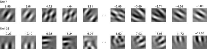
The corresponding eigenvalues are indicated above the eigenvectors.

Stimuli belonging to the space spanned by the eigenvectors with largest positive eigenvalues (i.e., all stimuli formed by a linear combination x = a1v1 + ⋯ aKvK of those eigenvectors) are thus going to elicit a strong response in the unit, and, conversely, points in the space spanned by those eigenvectors with largest negative eigenvalues are going to strongly inhibit the unit. This form of visualization has several problems. First, although the first and the last eigenvector typically have a very clear structure that is easy to interpret, the next ones very quickly look unstructured and do not lend themselves to an intuitive interpretation. Second, assume we are interested in the set of stimuli that yield a strong response of, say, more than 80% of the maximum response (given a certain stimulus energy). Some of the eigenvectors that would be discarded because they yield a response of less than 80% could still be necessary to generate stimuli that yield such a strong response (see Step 4 in the homogeneous case). Third, this method does not take into account the contribution of the linear term, which cannot generally be neglected5. The following steps describe an alternative method based on optimal stimuli and their invariances that does not suffer from these problems.
-
3
Compute the optimal stimuli x+ and x−. The optimal excitatory stimulus x+ (also called the 'preferred stimulus' in the literature) is defined as the input vector that maximizes the output of the model neuron given a fixed energy ‖x+‖ = r. The fixed energy constraint is necessary to make the problem well posed. Without such a constraint, arbitrarily high outputs can be generated if only the input is large enough in amplitude and points in a direction where the quadratic term is positive. This constraint is also the reason the quadratic form should be defined such that x = 0 is the neutral stimulus relative to which stimulus energy is measured. (As an alternative one could use the constraint ‖x − x′0‖ = r, with x′0 indicating the neutral stimulus, but this would clutter the analysis.) The optimal stimulus is thus defined by the following equations:
Maximize

under the constraint

It can be shown20 that the solution is unique in general and has the form x = (λ I − H)−1f, where λ is a scalar between μ1 and. ‖f‖/r+μ1 . The solution can therefore be found by searching over λ until Constraint 3.2 is satisfied.
The vector x and norm ‖x‖ can be efficiently computed for each λ using the expressions

and

The terms vi (viTf) and (viTf)2 are constant for a given quadratic form and can be computed in advance. As the norm of x is monotonically decreasing in the considered interval (Equation 3.4), the search can be performed efficiently using a simple bisection method. The pseudocode yielding the desired result is shown in Box 1. In the same way, it is possible to compute the optimal inhibitory stimulus x− by minimizing Equation (3.1), which is equivalent to maximizing −g(x). x− is the stimulus that most effectively inhibits the response of the unit.
Figure 2 shows optimal stimuli for units from the model simulation. If the quadratic form is homogeneous, the optimal excitatory stimulus points in the direction of the first eigenvector and is given by
Figure 2: Optimal excitatory and inhibitory stimuli for some of the units in the simulation. 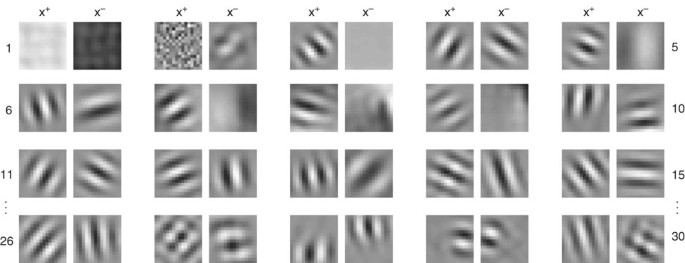
x+ looks similar to a Gabor wavelet in almost all cases, in agreement with physiological data. x− is usually structured and similar to a Gabor wavelet as well, which suggests that inhibition plays an important role. Units are numbered consecutively from 1 to 15 in the top four rows and from 26 to 30 in the last row.

In the same way, the optimal inhibitory stimulus is given by x− = ±r vN. This is one of the cases where the optimal stimuli are not unique but determined only up to the sign. If in addition the first eigenvalues were equal, any normalized linear combination of the corresponding eigenvectors would be an optimal stimulus.
-
4
Compute the invariances at x+ and x−. The optimal excitatory and inhibitory stimuli give us a first impression of the response properties of a unit and two anchor points at which we can refine the analysis. In this step we compute the invariances at the optimal stimuli, i.e., the transformations of x+ and x− to which the unit is most invariant. As in Step 3, we consider inputs of constant energy r, because otherwise a change in the response as we vary the direction of x around x+ could always be compensated by a change of length (i.e., energy) of x. Notice that around x+ the response can only drop and around x− it can only rise, because the optimal stimuli are extremal points. Mathematically we have to derive the quadratic form of g(x) constrained to the tangent space of the constant-energy sphere at x+ or x− and find the directions of smallest second derivative. In the following, we give the procedure for x+; x− can be treated analogously:
-
A
Apply the Gram–Schmidt orthogonalization algorithm to the vectors x+, e2, e3,...,eN, where ei is an element of the canonical basis; i.e., the i-th element of ei is one and the rest is zero (a simple implementation of this algorithm is included in the Matlab library, see MATERIALS). As a result, we obtain a basis b1,...,bN, where b1 = 1/rx+ and b2,...,bN are vectors orthogonal to it, which therefore form a basis of the space tangential to the sphere of radius r in x+. By restricting our computations to that space we locally enforce the constant energy constraint ‖x‖ = r. Define B: = (b2,...,bN)T.
-
B
Compute the directions of the invariances, which are given by the eigenvectors Ṽ of H̃ : = BT HB, ordered by decreasing eigenvalues ν1 ≥⋯≥νN−1. Project the eigenvectors back to the input space with

The second derivative in the direction of wi corresponds to the rate of change in the output caused by an infinitesimal movement from x+ in the wi direction. A small second derivative thus corresponds to a strong invariance. It is given by

which is non-positive, since x+ is a local maximum. The first term corresponds to the second derivative within the tangent space; the second term is a correction term, equal for all invariances, resulting from the fact that the movement is constrained to the surface of the sphere of constant energy (see ref. 20).
In the next step, we describe how to visualize the invariances, and in Steps 6 and 7 we discuss how to check which invariances are significant.
If the quadratic form is homogeneous, the invariances at x+ are given by the eigenvectors v2,...,vN in this order, and the second derivative on the sphere in the direction of vi is μi − μ1. The invariances at x− are given by vN−1,...,v2, with second derivatives μi − μN .
-
A
-
5
Visualize the significant invariances. To visualize invariance i in an animation, move the stimulus x around the optimal stimulus x+ (or x−) on the sphere of constant energy in the direction of wi along the path defined as

We recommend animating x(α) only within the range of α where the response maintains at least 80% of the maximal response (Fig. 3). Figure 4 shows three frames of such animations for six different invariances. The value of α at the extrema provides an indication of how robust the unit is to changes in that direction.
Figure 3: Illustration of the method used to visualize the invariances. 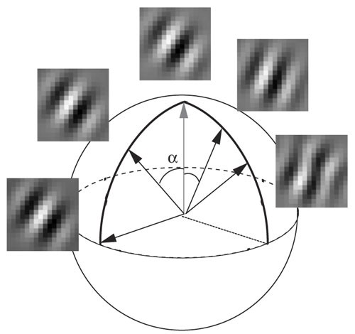
Starting from the optimal stimulus (top) we move on the sphere in the direction of an invariance until the response of the unit drops below 80% of the maximal output or reaches 90°. In the figure two invariances of Unit 4 are visualized. The one on the left represents a phase-shift invariance and preserves more than 80% of the maximal output until 90° (the output at 90° is 99.6% of the maximum). The one on the right represents an invariance to orientation change. The output drops below 80% at 55°.
Figure 4: Example invariances at the optimal stimuli for some of the units. 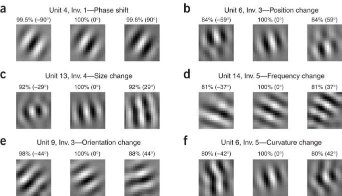
The central patch of each plot represents the optimal stimulus for a unit, and the ones on the sides are produced by moving it in one (left path) or the other (right patch) direction of the eigenvector corresponding to the invariance. To produce this plot, we stopped before the output dropped below 80% of the maximum to make the interpretation of the invariances easier. The relative output of the function as a percentage and the angle of displacement α (eqn. 5.1) are given above the patches. The animations corresponding to these invariances are available at the authors' homepages.
-
6
Collect random quadratic forms. To assess which of the invariances computed in the preceding step are statistically significant, we compare them to those of random quadratic forms with similar output statistics, which are generated in this step. Perform Option (A) for theoretical simulations and Option (B) for physiological experiments.
-
A
In theoretical simulations
In many theoretical studies, one enforces a fixed mean and variance on the output of the units. Without loss of generality, we assume here zero mean and unit variance, which can be achieved as follows:
-
i
Expand the input data in the space of polynomials of degree two using the mapping

-
ii
Compute the mean of the expanded data

and the eigenvalue diagonal matrix Λ and eigenvector matrix E of the covariance matrix

-
iii
Compute the whitening matrix S = Λ−1/2ET.
-
iv
Generate random vectors qi′ of length 1 in the whitened, expanded space and derive the corresponding quadratic forms in the original input space using the relation

with qi:=STqi′ and c := qTjφ̇. The output of the resulting random quadratic forms has zero mean and unit variance by construction.
Critical Step
The random vectors of length 1 must be uniformly distributed on the unit sphere. This can be easily achieved by repeatedly drawing random numbers from a zero-mean Gaussian distribution, arranging them in a vector and then normalizing the vector to norm 1. It is important not to use random numbers from a uniform distribution, because that would introduce a strong bias toward the corners of the unit cube.
-
i
-
B
In physiological experiments
-
i
In physiological experiments, random quadratic forms can be generated by bootstrapping. The spikes can be shuffled6,10 or the entire spike train can be shifted relative to the stimulus sequence9,12 (this second possibility is to be preferred if the input stimuli have a temporal structure, i.e., a non-zero autocorrelation) and the same RF estimation procedure used to generate the units under consideration can be applied to the resulting data. The new randomly generated quadratic forms are compatible with the distribution of the input data and with the total number of spikes elicited in the neuron under consideration.
-
i
-
A
-
7
Compute confidence interval. Estimating a confidence interval for the invariances is difficult because of their interdependencies (we have an ordered set of invariances and not independent invariances) and because it is not clear what a good model of the background distribution is against which significance can be judged. We have, therefore, adopted a rather heuristic approach, as follows20. Compute the optimal stimuli and second derivatives of the invariances of the random quadratic forms as in Steps 3 and 4. Keep one randomly chosen second derivative per quadratic form to ensure the measurements are independent. This allows us to determine a distribution over the random second derivatives and a corresponding 95% confidence interval, which yields a significance threshold for the second derivatives of the learned units. Figure 5 shows that, in the model simulation, this threshold coincides with the value at which the distribution of the learned second derivatives changes from a rather Gaussian distribution on the left to a more structured distribution on the right, which we take as an additional hint that the threshold is reasonable.
Figure 5: Significant invariances. 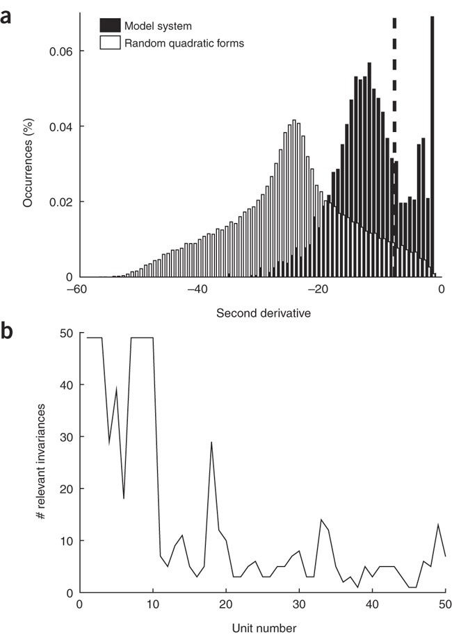
(a) Distribution of 50,000 independently drawn second derivatives of the invariances of random quadratic forms and distribution of the second derivatives of all invariances of the first 50 units in the simulation. The dashed line indicates the 95% confidence limit. Of all invariances, 28% were classified as significant. (b) Number of significant invariances for each of the first 50 units learned in the simulation (the units are sorted by decreasing slowness).


Anticipated results
In the following, we present the outcome of the analysis procedure described above when applied to the results of the model simulation reported in ref. 1. In that study, we applied a computational model of V1 based on the temporal slowness principle21 to natural-image-patch sequences, which yielded a set of quadratic forms representing non-linear RFs of visual neurons. The resulting units had the primary characteristics of complex cells in V1, namely, Gabor-like optimal stimuli and phase-shift invariance, as well as a number of secondary behaviors, such as end and side inhibition, direction selectivity and non-orthogonal inhibition. The results of another, more detailed simulation have been reported elsewhere2.

Step 2
The eigenvectors of Units 4 and 28 are shown in Figure 1, ordered by decreasing eigenvalues. In Unit 4, the first two eigenvectors look similar to Gabor wavelets with a 90° phase difference. As the two eigenvalues have almost the same magnitude, the response of the quadratic term is similar for the two eigenvectors and also for linear combinations thereof with constant norm 1. For this reason, this unit responds strongly to edges or gratings but is invariant to changes in the phase or exact position of the stimulus and thus has the defining characteristics of complex cells in V1. The last two eigenvectors, which correspond to stimuli that minimize the quadratic term, are Gabor wavelets with an orientation orthogonal to that of the first two. As a consequence, the output of the quadratic term is inhibited by stimuli with an orientation orthogonal to the preferred one. In the case of Unit 28, the first and the last two eigenvalues have the same orientation but occupy two different halves of the RF. This means that Unit 28 is end inhibited; i.e., an extension of the length of an optimally oriented sine grating beyond the excitatory half of the RF into the inhibitory half leads to a decrease in response as opposed to a saturation as in conventional cells.
A direct interpretation of the remaining eigenvectors in the two units is difficult, although the magnitude of the eigenvalues shows that some of them elicit a strong response. Moreover, the interaction of the linear and quadratic terms to form the overall output of the quadratic form is not considered but cannot be neglected in general5 (even though it is small for the two units considered here). We show below that the optimal stimuli and the respective invariances can be more easily visualized and interpreted when the linear term is taken into account.
Step 3
Figure 2 shows the optimal excitatory and inhibitory stimuli of some of the units in the simulation. In almost all cases, x+ looks similar to a Gabor wavelet, in agreement with physiological data for neurons in V1 (ref. 22). x− is usually structured as well, which suggests that inhibition also plays an important role in shaping the response of the unit. As in these two cases the linear term is negligible20, the optimal stimuli of Units 4 and 28 are almost identical to the eigenvectors of largest magnitude (compare Fig. 1, first and last eigenvectors, with Fig. 2, Units 4 and 28). However, for quadratic forms with a significant linear term this does not need to be the case.
Steps 4–7
Figure 4 shows animations corresponding to some representative invariances. The animations show that the behavior of the units is more complex than suggested by the eigenvectors alone. They have active mechanisms to shape their orientation and frequency bandwidths and some have a limited invariance to changes in curvature (this characteristic is often associated with end or side inhibition). Figure 5a shows the distribution of 50,000 independent second derivatives of the invariances of random quadratic forms and that of the first 50 units learned in the simulation. The latter is clearly skewed toward zero (i.e., toward more invariant directions) and has a peak near zero. Of all invariances, 28% were classified as significant according to the 95% confidence interval for the random quadratic forms (dashed line). Figure 5b shows the number of significant invariances for the individual units (each unit has 49 invariances in total). Of 50 units, 46 have three or more significant invariances. The first invariance corresponds in all cases to a phase-shift invariance and was always classified as highly significant (P < 0.0005), which confirms that the units behave in a similar way to complex cells.
References
Berkes, P. & Wiskott, L. Applying slow feature analysis to image sequences yields a rich repertoire of complex cell properties. In Artificial Neural Networks-ICANN 2002 Proceedings, Lecture Notes in Computer Science (ed. Dorronsoro, J.R.) 81–86 (Springer, Berlin, 2002).
Berkes, P. & Wiskott, L. Slow feature analysis yields a rich repertoire of complex cell properties. J. Vis. 5, 579–602 (2005).
Marmarelis, P. & Marmarelis, V. Analysis of physiological systems: the white-noise approach (Plenum Press, New York, 1978).
de Ruyter van Steveninck, R. & Bialek, W. Real-time performance of a movement-sensitive neuron in the blowfly visual system: coding and information transfer in short spike sequences. Proc. R. Soc. Lond. B Biol. Sci. 234, 379–414 (1988).
Lewis, E.R., Henry, K.R. & Yamada, W.M. Tuning and timing in the gerbil ear: Wiener-kernel analysis. Hear. Res. 174, 206–221 (2002).
Touryan, J., Lau, B. & Dan, Y. Isolation of relevant visual features from random stimuli for cortical complex cells. J. Neurosci. 22, 10811–10818 (2002).
Rust, N.C., Schwartz, O., Movshon, J.A. & Simoncelli, E.P. Spike-triggered characterization of excitatory and suppressive stimulus dimensions in monkey V1. Neurocomp. 58–60, 793–799 (2004).
Simoncelli, E.P., Paninski, L., Pillow, J.W. & Schwartz, O. Characterization of neural responses with stochastic stimuli. In The Cognitive Neurosciences 3rd edn. (ed. Gazzaniga, M.S.) 327–338 (MIT Press, Cambridge, Massachusetts, 2004).
Rust, N.C., Schwartz, O., Movshon, J.A. & Simoncelli, E.P. Spatiotemporal elements of macaque V1 receptive fields. Neuron 46, 945–956 (2005).
Touryan, J., Felsen, G. & Dan, Y. Spatial structure of complex cell receptive fields measured with natural images. Neuron 45, 781–791 (2005).
Rapela, J., Mendel, J.M. & Grzywacz, N.M. Estimating nonlinear receptive fields from natural images. J. Vis. 4, 441–474 (2006).
Schwartz, O., Pillow, J.W., Rust, N.C. & Simoncelli, E.P. Spike-triggered neural characterization. J. Vis. 6, 484–507 (2006).
Franz, M.O. & Schölkopf, B. A unifying view of Wiener and Volterra theory and polynomial kernel regression. Neural Comput. 18, 3097–3118 (2006).
Hashimoto, W. Quadratic forms in natural images. Netw. Comput. Neural Syst. 14, 765–788 (2003).
Bartsch, H. & Obermayer, K. Second-order statistics of natural images. Neurocomp. 52–54, 467–472 (2003).
Hyvärinen, A. & Hoyer, P. Emergence of phase- and shift-invariant features by decomposition of natural images into independent feature subspaces. Neural Comput. 12, 1705–1720 (2000).
Hyvärinen, A. & Hoyer, P. A two-layer sparse coding model learns simple and complex cell receptive fields and topography from natural images. Vision Res. 41, 2413–2423 (2001).
Körding, K.P., Kayser, C., Einhäuser, W. & König, P. How are complex cell properties adapted to the statistics of natural stimuli? J. Neurophysiol. 91, 206–212 (2004).
Adelson, E.H. & Bergen, J.R. Spatiotemporal energy models for the perception of motion. J. Opt. Soc. Am. A 2, 284–299 (1985).
Berkes, P. & Wiskott, L. On the analysis and interpretation of inhomogeneous quadratic forms as receptive fields. Neural Comput. 18, 1868–1895 (2006).
Wiskott, L. & Sejnowski, T.J. Slow feature analysis: unsupervised learning of invariances. Neural Comput. 14, 715–770 (2002).
Jones, J.P. & Palmer, L.A. An evaluation of the two-dimensional Gabor filter model of simple receptive fields in cat striate cortex. J. Neurophysiol. 58, 1233–1257 (1987).
Acknowledgements
The figures have been reproduced with permission from ref. 20. This work has been supported by a grant to L.W. from the Volkswagen Foundation and by the Gatsby Charitable Foundation.
Author information
Authors and Affiliations
Corresponding author
Ethics declarations
Competing interests
The authors declare no competing financial interests.
Rights and permissions
About this article
Cite this article
Berkes, P., Wiskott, L. Analysis and interpretation of quadratic models of receptive fields. Nat Protoc 2, 400–407 (2007). https://doi.org/10.1038/nprot.2007.27
Published:
Issue Date:
DOI: https://doi.org/10.1038/nprot.2007.27
This article is cited by
-
On solving trust-region and other regularised subproblems in optimization
Mathematical Programming Computation (2010)
Comments
By submitting a comment you agree to abide by our Terms and Community Guidelines. If you find something abusive or that does not comply with our terms or guidelines please flag it as inappropriate.
