The methodology of design of satellite working mechanism of positive displacement machine

Abstract

In this paper is described a methodology of design of satellite mechanism consisting of two non-circular gears (externally toothed rotor and internally toothed curvature) and circular gears (satellites). In the presented methodology is assumed that the rotor pitch line is known, and the curvature pitch line is necessary to designate. The presented methodology applies to mechanisms for which the number of the curvature humps is at least one greater than the number of rotor humps. The selection of the number of gears and the number of teeth in gear and rotor and curvature is also presented. The methodology of calculating the position of the satellite center and the angle of its rotation in order to shape the teeth on the rotor and curvature is presented. The article is also showed different types of satellite mechanisms—satellite mechanisms with the different numbers of humps on the rotor and curvature. The technical parameters of the mechanism for the rotor pitch line described by the cosine function are also presented.

Introduction

In hydrostatic drive systems, positive displacement machines are pumps and hydraulic motors. Due to high operating pressures, piston pumps and piston motors dominate in hydrostatic systems^1,2,3,4,5. Other constructions of positive displacement machines, such as gear^6,7,8,9,10, gerotor¹¹ or vane machines¹², are also used. Recent years have been a period of intensive development of positive displacement machines, especially hydraulic motors, in which the working mechanism is a special set of non-circular gears. This article is devoted to these machines.

The idea of non-circular gears is not new. Non-circular gears were used in many devices to provide irregular motion, which is the transfer (generally) stable input velocity into various output velocities. An example of such devices are clockworks, astronomical devices, electromechanical systems to control and drive non-linear potentiometers, textile machines¹³, mechanical presses^14,15,16 and mechanical toys also. Furthermore, from the eighteenth century, the non-circular gears were commonly used in positive displacement machines like in pumps and in flowmeters (Fig. 1)¹⁷. Both gear transmissions and hydraulic positive displacement machines (Fig. 1) are built with non-circular gears with a constant distance between the axles of these wheels. The methods of designing such gear transmissions are widely described in the literature^{13,14,15,16,17,18,19,20,21,22,23}.

Figure 1

Non-circular gears in positive displacement machine¹⁷.

While at the end of the nineteenth century the first hydraulic motor with non-circular gears was built^24,25,26. This motor was called satellite motor (Fig. 2).

Figure 2

The working mechanism of the first satellite motor (type 3 × 4): 1—rotor, 2—curvature, 3—satellite^24,25,26.

The conception of satellite motor working mechanism is based on mutual cooperation of the external toothed non-circular wheel (called rotor) with the internal toothed non-circular wheel (called curvature) through the round gears (called satellites) between them. The satellites play the role of movable, inter-chamber partitions. Simultaneously, the satellite functions as inflow and outflow dividers when the working chamber passes from the filling phase to the extrusion phase²⁶.

By the type of the satellite mechanism should be understood its characteristic feature, which is the number n_R of humps on the rotor and the number n_E of humps on the curvature. Thus, the type of mechanism will be marked as “n_R x n_E”.

Currently, hydraulic motors with four types of satellite mechanisms are manufactured (Figs. 2, 3i, 4).

Figure 3

Satellite mechanisms: type 4 × 6 (left) and type 6 × 8 (right): 1—rotor, 2—curvature, 3—satellite^{26,28,29,30,31,32,33,34}.

Figure 4

The hydraulic motor with satellite mechanism type 4 × 5. The number of teeth: curvature z_E = 130, rotor z_R = 104 and satellite z_S = 12, tooth module m = 0,5 mm^35,36.

Satellite mechanisms are used not only to build a hydraulic motor, but also to build a pressure intensifier and a pump^36,37,38,39.

According to patents^30,31,34, the shape of the rotor consists of arcs of circles with different radii and tangents to each other. Similarly, the shape of the curvature is the sum of arcs with different radii. These constructions resulted mainly from the available technologies of their production. Both the teeth of the rotor and the curvature were made by diagonal hobbing with a Fellows tool with the use of special tooling of a slotting machine^40,41,42. While the satellites were made using the milling method. Therefore, when designing a satellite mechanism, the available tools (number of chisel teeth, its diameter etc.) should also be taken into account. Moreover, the phenomenon of tooth interference in the mechanism had to be avoided⁴³. Therefore, Kujawski in⁴³ formed the rotor of the type 4 × 6 mechanism by the arcs of circles connected by straight sections and the construction of curvature consists of only arcs of circles. Kujawski was the first to present the guidelines and basics of designing the satellite mechanisms⁴³.

In work²⁶ a four-humped rotor is composed of arcs tangent to each other are presented (Fig. 5). Dowel Li et al. also developed a methodology of designing the satellite mechanism type 4 × 6 based on circular arc curves of the rotor and curvature⁴⁴.

Figure 5

Rotor (four-humped) as a sum of arcs²⁶.

In mechanisms type 3 × 4, 4 × 6 and 6 × 8 the shape of the rotor consists of arcs of circles with different radii and tangents to each other. It was shown in²⁶ that in these mechanisms are unfavourably large changes in the satellite’s acceleration at the moment of transition from the convex part of rotor to the concave part, i.e. in point where arcs of circles meet (Fig. 6). The immediate cause of this is a jump change in the radius value at the point of tangency of the circle’s arcs. Thus, in an operating mechanism, especially at high rotational speed, there will be a large mechanical loss which contributes to accelerated wear of the teeth. Figure 7 shows that the wear occurs not only at the points of contact of the arcs but also on the convexity (on the hump) of the rotor. The reason for this is the small radius of this hump⁴⁵.

Figure 6

The characteristic of the angular acceleration of satellite in mechanism type 4 × 6 (at the angular speed of rotor ω = 10 rad/s)²⁶.

Figure 7

Specific wear of the teeth on the humps of the rotor. Working liquid—emulsion HFA-E. Unknown mechanism operation time^26,45.

Currently is possible to manufacture the toothed elements using the wire electrical discharge machining (the so-called WEDM method). This method is already used to manufacture well-known satellite mechanisms, especially the 4 × 6 type, the structures of which were designed to be made by chiseling^44,47,48. Thus, the WEDM makes it possible to manufacture satellite mechanisms with different rotors and curvature shapes. For example, the rotor of the mechanism type 4 × 5 (Fig. 4) has a circular-sinusoidal shape³⁵. The radius r_R of the rotor pitch line was described by equation³⁵:

$${\mathrm{r}}_{\mathrm{R}}={\mathrm{r}}_{\mathrm{Rmin}}+\frac{{\mathrm{r}}_{\mathrm{Rmax}}-{\mathrm{r}}_{\mathrm{Rmin}}}{2}\cdot \left(1+\mathrm{cos}\left({\mathrm{n}}_{\mathrm{R}}\cdot {\mathrm{\alpha }}_{\mathrm{R}}+\uppi \right)\right)$$

(1)

where r_Rmin and r_Rmax—respectively: minimum and maximum rotor radius, n_R—the number of the rotor humps, α_R—angle (Fig. 13).

For the mechanism shown in Fig. 4 is: r_Rmin = 22,552 mm and r_Rmax = 27.524 mm³⁵.

Nowadays are proposed the next concepts of satellite mechanism. Osiecki proposes a satellite mechanism type 2 × 4 with the elliptical shape of the rotor (two humps) and with four humps curvature^45,46. However, Osiecki did not disclose the methodology of designing curvature and methodology of selection the number of teeth in the mechanism elements (rotor, curvature and satellite). In literature the satellite mechanisms type 2 × 2 and 2 × 3 are also known (Fig. 8)^{49,50,51,52,53,54,55,56}.

Figure 8

Satellite mechanisms: type 2 × 2 (left), type 2 × 3 (middle) and type 2 × 4 (right), 1—rotor, 2—satellite, 3—curvature^{49,50,51,52,53,54,55,56}.

Volkov at all propose to design satellite mechanisms, like shown in Fig. 8, by specifying, first, the trajectory of the satellite’s center associated with the rotor and with the curvature. In polar coordinates the distance L_SR of the satellite center associated with the rotor from the origin of the coordinate system is^49,50,51,52:

$${\mathrm{L}}_{\mathrm{SR}}={\mathrm{L}}_{\mathrm{c}}\cdot \left(1+{\mathrm{k}}_{t}\cdot \mathrm{f}\left({\mathrm{n}}_{\mathrm{R}}\cdot {\mathrm{\alpha }}_{\mathrm{SR}}\right)\right)$$

(2)

and the distance L_SE of the satellite center associated with the curvature from the origin of the coordinate system is^49,50,51,52:

$${\mathrm{L}}_{\mathrm{SE}}={\mathrm{L}}_{\mathrm{c}}\cdot \left(1+{\mathrm{k}}_{t}\cdot \mathrm{f}\left({\mathrm{n}}_{\mathrm{E}}\cdot {\mathrm{\alpha }}_{\mathrm{SE}}\right)\right)$$

(3)

where f(…)—cyclic function, k_t—the coefficient that characterizes the non-circularity of the trajectories, L_C—the radius of the circle to which both trajectories degenerate when k = 0, α_SR and α_SE—polar angles associated with the rotor and curvature respectively.

Next, the rotor and curvature curves are calculated as equidistance’s of the above-mentioned trajectories (2) and (3), assuming the satellite diameter and the number of teeth on the satellite, rotor and curvature^49,50,51,52.

Zhang et al.⁵⁷ and Wang et al.³⁹ propose the new satellite mechanism type 4 × 6 with the high-order ellipse shape of the rotor. The pitch curve of the rotor is described in polar coordinates as:

$${\mathrm{r}}_{\mathrm{R}}=\frac{A\cdot \left(1-{k}^{2}\right)}{1+{\mathrm{k}}_{e}\cdot \mathrm{cos}\left({n}_{R}\cdot {\mathrm{\alpha }}_{\mathrm{R}}-\pi \right)}$$

(4)

where r_R—the distance between the origin of the coordinate system and a point on the rotor pitch curve, k_e—the eccentricity of the ellipse, A—the long-axis radius of the ellipse, α_R—the polar angle of the rotor pitch curve.

Zhang at all are also propose to describe the rotor pitch line as⁵⁷:

$${\mathrm{r}}_{\mathrm{R}}={\mathrm{A}}_{h}\cdot \mathrm{cos}\left({n}_{R}\cdot {\mathrm{\alpha }}_{\mathrm{R}}\right)+B\cdot \mathrm{cos}\left(2\cdot {n}_{R}\cdot {\mathrm{\alpha }}_{\mathrm{R}}\right)+{\mathrm{r}}_{\mathrm{c}}$$

(5)

where r_c—the radius of basic circle, A_h—the amplitude of the cousine function, B—coefficient.

According to Zhang, Wang at all the equation describing the curvature pitch curve in polar coordinates is^39,57:

$${\mathrm{r}}_{\mathrm{E}}={\mathrm{r}}_{\mathrm{R}}+2\cdot \frac{{\mathrm{r}}_{\mathrm{R}}\cdot {\mathrm{r}}_{\mathrm{S}}}{{\left[{{\mathrm{r}}_{\mathrm{R}}}^{2}+{\left(\frac{d{\mathrm{r}}_{\mathrm{R}}}{d{\mathrm{\alpha }}_{\mathrm{R}}}\right)}^{2}\right]}^{\mathrm{0,5}}}$$

(6)

$${\mathrm{\alpha }}_{\mathrm{E}}={\int }_{0}^{{\mathrm{\alpha }}_{\mathrm{R}}}\left[{\mathrm{r}}_{\mathrm{R}}+2\cdot \frac{{\mathrm{r}}_{\mathrm{R}}\cdot {\mathrm{r}}_{\mathrm{S}}}{{\mathrm{r}}_{\mathrm{E}}}\cdot \frac{{\left(\frac{d{\mathrm{r}}_{\mathrm{R}}}{d{\mathrm{\alpha }}_{\mathrm{R}}}\right)}^{2}-{\mathrm{r}}_{\mathrm{R}}\cdot \frac{{d}^{2}{\mathrm{r}}_{\mathrm{R}}}{d{{\mathrm{\alpha }}_{\mathrm{R}}}^{2}}}{{\left[{{\mathrm{r}}_{\mathrm{R}}}^{2}+{\left(\frac{d{\mathrm{r}}_{\mathrm{R}}}{d{\mathrm{\alpha }}_{\mathrm{R}}}\right)}^{2}\right]}^{\mathrm{1,5}}}\right]d{\mathrm{\alpha }}_{\mathrm{R}}$$

(7)

where r_E—the distance between the origin of the coordinate system and a point on the curvature pitch curve, r_S—radius of the satellite pitch curve, α_E—the polar angle of the curvature pitch curve.

Zhang at all indicate that with an inapproprioprate selection of parameters, the curvature is characterized by self-interlacing of the pitch line (Fig. 9) or by undercutting the teeth (Fig. 10).

Figure 9

The phenomenon of self-interlacing of the curvature pitch line⁵⁷.

Figure 10

The phenomenon of undercutting the curvature teeth⁵⁷.

Furthermore, Zhang at all indicate, when selecting the pitch curve parameters, it is necessary to draw the tooth profile of each gear at the same time to judge its feasibility⁵⁷. It is a certain inconvenience. The next problem to solve is determining how to select the coefficients A_h and B in Eq. (5) in solving the undercutting problem of the curvature so that the number of satellite teeth z_S is small enough⁵⁷.

In the above-characterized known methods of designing a satellite mechanism, some disadvantages related to the selection of the parameters of the rotor and curvature pitch lines as well as the selection of the number of teeth and their module can also be seen. Therefore, new two methods for designing any type of satellite mechanism for n_E > n_R are proposed below. The first method allows determining parameters of satellite mechanism for the perfect solution and the second method allows for the correction of the teeth.

Proposed method of designing a satellite mechanism

In the method of designing a satellite mechanism it is assumed that the satellite plays the role of a chisel. That is in a computer program the satellite chisels the gears of the rotor and curvature. Therefore, the mathematical relationships describing the position of the satellite center in the X–Y coordinate system and the corresponding angle of satellite rotation are also presented below.

Basic conditions

It is assumed that for each radius r_s of the satellite’s pitch circle and for each rotor pitch line exists a corresponding to them a pitch line of curvature, which fulfils the conditions of perfect cooperation. These conditions are as follows⁴³:

• (a) in each mutual position of rotor and curvature, obtained as a result of the rotation of one of them around the other, the pitch circles of all satellites must be tangent to the pitch lines of the rotor and the curvature;

• (b) the pitch circles of all satellites must pitch without slipping on the pitch lines of the rotor and the curvature;

• (c) on all length of rotor’s pitch line and on all length of the curvature’s pitch line must exist such humps that make the possible pitch of the satellite’s pitch circle on the external side of the rotor’s pitch line and on the internal side of the curvature’s pitch line;

• (d) the rotors and curvature’s pitch lines should be cyclically changing curves and must not overlap with mutual rotational displacement;

• (e) the centers S of the satellites should be located at the intersection point of the equidistant e_R of the pitch line of the rotor with the equidistant e_E of the pitch line of the curvature (equidistance are the tracks of the satellite centers, which arise as a result of the pitch the satellite on the pitch lines of the rotor and the curvature) (Fig. 11);

  Figure 11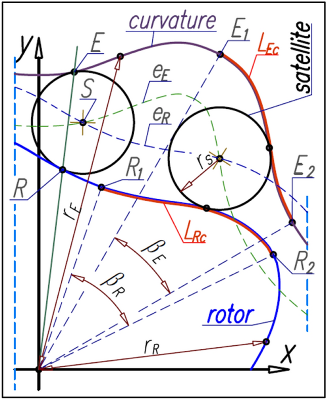

  

  The basic geometrical relationships in satellite mechanism.

• (f) the point R of contact of the satellite with the rotor and the point E of contact of the satellite with the curvature lie on a straight line that passes through the center of rotation of the rotor and curvature (Fig. 11);

• (g) if the curves of the rotor are between points R₁ and R₂ and the curves of curvature are between points E₁ and E₂ (Fig. 11) and also the tangents to these curves are perpendicular to the leading radii r_R (rotor) and r_E (curvature) then the length L_Rc of the basic curve of the rotor is equal to the length L_Ec of the basic curve of curvature:

  $${\mathrm{L}}_{\mathrm{Rc}}={\mathrm{L}}_{\mathrm{Ec}}$$

  (8)

• (h) the central angle β_R that covers one half of the cycle of the rotor pitch curve (corresponding to length L_Rc) is:

  $${\upbeta }_{\mathrm{R}}=\frac{\uppi }{{\mathrm{n}}_{\mathrm{R}}}$$

  (9)

  where n_R is the number of the rotor humps;

• (i) the central angle β_E that covers one half of the cycle of the curvature’s pitch curve (corresponding to length L_Ec) is:

  $${\upbeta }_{\mathrm{E}}=\frac{\uppi }{{\mathrm{n}}_{\mathrm{E}}}$$

  (10)

  where n_E is the number of the curvature humps;

• (j) the number of humps of the curvature is greater than the number of humps of the rotor (n_E > n_R).

Proposed sequence of proceeding during the design

When starting the design of the satellite mechanism, the first step is to take the number of humps n_R on the rotor and the number of humps n_E on the curvature. Next the radius r_c of the rotor basic circle must be chosen.

When designing a satellite mechanism it should be remembered that:

• (a) the number of teeth z_Rc in the range of rotor angle β_R (Fig. 16) is:

  $${\mathrm{z}}_{\mathrm{Rc}}=\frac{{\mathrm{L}}_{\mathrm{Rc}}}{\uppi \cdot \mathrm{m}}$$

  (11)

• (b) because the condition (8) must be met, then:

  $${\mathrm{z}}_{\mathrm{Ec}}={\mathrm{z}}_{\mathrm{Rc}}$$

  (12)

• (c) the number of teeth z_R on the rotor is:

  $${\mathrm{z}}_{\mathrm{R}}=2\cdot {\mathrm{n}}_{\mathrm{R}}\cdot {\mathrm{z}}_{\mathrm{Rc}}$$

  (13)

• (d) the number of teeth z_E on the curvature is:

  $${\mathrm{z}}_{\mathrm{E}}=2\cdot {\mathrm{n}}_{\mathrm{E}}\cdot {\mathrm{z}}_{\mathrm{Rc}}$$

  (14)

• (e) numbers of teeth z_R and z_E must be integer;

• (f) the number of teeth 2z_Rc on the rotor hump (and the same on the curvature hump) must be an integer. Otherwise, despite the fulfilment of the condition (8) and the total number of rotor teeth z_R and curvature teeth z_E, the satellite mechanism cannot be assembled correctly. An example of such mechanism is presented in Fig. 12.

Figure 12

Satellite mechanism type 4 × 6 with incorrectly selected parameters: z_S = 9, z_Rc = 4.75, z_R = 38, z_E = 57. Every second satellite cannot be inserted into the mechanism.

The first method: searching for the perfect solution

Having the number of humps n_R and n_E should be sequentially:

• 1. to adopt radius r_c of rotor basic circle;

• 2. using the iteration method should be searched the amplitude A_h and the satellite radius r_S until the condition (8) is met with simultaneous fulfilment of the condition (54);

• 3. using the iteration method should be searched the number of satellite teeth z_S so that the numbers of teeth z_R and z_E are integer;

• 4. to calculate teeth module m according to the following formula:

  $$\mathrm{m}=2\cdot \frac{{\mathrm{r}}_{\mathrm{S}}}{{\mathrm{z}}_{\mathrm{S}}}$$

  (15)

  The calculated value of module m does have to correspond to the normalized value;

• 5. to adopt the desired normalized value of module m_st;

• 6. all the parameters of the satellite mechanism should be scaled by a value:

  $$\mathrm{i}=\frac{\mathrm{m}}{{\mathrm{m}}_{\mathrm{St}}}$$

  (16)

The search for the parameters of satellite mechanism, ie A_h, r_S and z_S so that the condition (54) was met may prove impossible. Then it is worth to allowing a certain difference δ of the lengths L_Rc and L_Ec, but not greater than the limit value δ_b, that is:

$$\left|{\mathrm{L}}_{\mathrm{Rc}}-{\mathrm{L}}_{\mathrm{Ec}}\right|=\updelta \le {\updelta }_{\mathrm{b}}$$

(17)

The value δ_b is justified, for example, by the fact that depending on the processing technology, different accuracy of the manufacturing of satellite mechanism elements is obtained.

The second method

Having the number of humps n_R and n_E should be sequentially:

• 1. to adopt the basic circle radius r_c of the rotor;

• 2. to adopt the amplitude A_h;

• 3. by iteration method to search the satellite radius r_S until the condition (8) is met while meeting the condition (54) (presented in “Method 2”);

• 4. to adopt the number of teeth z_Rc (keeping in mind that the number of teeth 2z_Rc on the rotor hump should be integer);

• 5. to calculate module m by transforming the formula (11);

• 6. to calculate the number of teeth z_S by transforming the formula (15). The obtained value z_S need not be an integer;

• 7. if the calculated value of z_S is not integer then the total number of the satellite teeth z_Sst should be adopted. It is recommended that:

  $$\left|{\mathrm{z}}_{\mathrm{S}}-{\mathrm{z}}_{\mathrm{Sst}}\right|=\mathrm{min}$$

  (18)
  $${\mathrm{z}}_{\mathrm{Sst}}<{\mathrm{z}}_{\mathrm{S}}$$

  (19)

• 8. to apply the P-O correction of the teeth. The minimum value of the correction coefficient is:

  $${\mathrm{x}}_{\mathrm{smin}}=\frac{{\mathrm{z}}_{\mathrm{S}}-{\mathrm{z}}_{\mathrm{Sst}}}{2}$$

  (20)

• 9. in order to generate corrected teeth of the rotor and the curvature, the angle γ_Sst of satellite rotation relative to its center S should be calculated according to the following formula:

  $${\upgamma }_{\mathrm{Sst}}=\frac{{\mathrm{L}}_{\mathrm{R}}}{{\mathrm{r}}_{\mathrm{Sst}}}+\mathrm{arctan}\left(\frac{{\mathrm{x}}_{\mathrm{R}}-{\mathrm{x}}_{\mathrm{S}}}{{\mathrm{y}}_{\mathrm{R}}-{\mathrm{y}}_{\mathrm{S}}}\right)$$

  (21)

  where:

  $${\mathrm{r}}_{\mathrm{Sst}}=\mathrm{m}\cdot \frac{{\mathrm{z}}_{\mathrm{Sst}}}{2}$$

  (22)

Rotor designing: the coordinates of the rotor pitch line

According to the basic conditions shown in “Basic conditions” the rotor’s pitch lines should be a cyclically changing curve. Furthermore, the rotor should have a total number of humps n_R evenly distributed over the entire circumference of the rotor. Therefore, the radius r_R of the rotor pitch line can be defined by any cyclical function type r_R = f(α_R), for example functions (1), (4), (5) and any others. A schematic sketch of a quarter rotor with the basic geometrical dimensions is shown in Fig. 13.

Figure 13

The basic parameters of the rotor.

The coordinates (x_R,y_R) of the point R on the rotor pitch line are:

$${\mathrm{x}}_{\mathrm{R}}={\mathrm{r}}_{\mathrm{R}}\cdot \mathrm{sin}{\mathrm{\alpha }}_{\mathrm{R}}$$

(23)

$${\mathrm{y}}_{\mathrm{R}}={\mathrm{r}}_{\mathrm{R}}\cdot \mathrm{cos}{\mathrm{\alpha }}_{\mathrm{R}}$$

(24)

The most distant point of the rotor pitch line from the center of rotation of this rotor (i.e. from the origin of the coordinate system) designates the straight-line k which is the axis of symmetry of the rotor hump (Fig. 13). If α_S = α_R = β_R then the satellite center S and the tangent point R of the satellite with the rotor lie on the straight-line k (Fig. 16b). The angle β_R can be calculated from the formula (10).

The coordinates of the satellite center

The satellite pitch circle with radius r_s must be tangent in the point R to the rotor pitch line (Fig. 14).

Figure 14

The coordinates of the satellite center.

The coordinates (x_S,y_S) of the satellite center S can be calculated according to the following formulas:

$${\mathrm{x}}_{\mathrm{S}}={\mathrm{x}}_{\mathrm{R}}\pm {\mathrm{r}}_{\mathrm{S}}\cdot \frac{1}{\sqrt{{1+{\mathrm{a}}_{\left(\mathrm{R}\right)\mathrm{p}}}^{2}}}$$

(25)

$${\mathrm{y}}_{\mathrm{S}}={\mathrm{y}}_{\mathrm{R}}\pm {\mathrm{r}}_{\mathrm{S}}\cdot \frac{{\mathrm{a}}_{\left(\mathrm{R}\right)\mathrm{p}}}{\sqrt{{1+{\mathrm{a}}_{\left(\mathrm{R}\right)\mathrm{p}}}^{2}}}$$

(26)

where a_(R)p is the slope of the straight-line y_(R)p perpendicular to the tangent line y_(R)t in the point R (Fig. 14). If a_(R)p < 0 then in formulas (25) and (26) is a “−” sign instead of the “±” sign. But for a_(R)p ≥ 0 is sign “+”.

The angular position of the satellite center S (angle α_S in Fig. 14) about the axis OY can be calculated from the following formula:

$${\mathrm{\alpha }}_{\mathrm{S}}=\mathrm{arctan}\left(\frac{{\mathrm{x}}_{\mathrm{S}}}{{\mathrm{y}}_{\mathrm{S}}}\right)$$

(27)

whereas the distance L_S of satellite center S from the origin of the coordinate system is:

$${\mathrm{L}}_{\mathrm{S}}=\sqrt{{\mathrm{x}}_{\mathrm{S}}^{2}+{\mathrm{y}}_{\mathrm{S}}^{2}}$$

(28)

The angle of satellite rotation

Each position of satellite center S described by formulas (25) and (26) is assigned the angle γ_S of the satellite rotation around the center S (Fig. 15).

Figure 15

Angles of the satellite.

The angle γ_S of satellite rotation around its center S can be calculated according to the following formula:

$${\upgamma }_{\mathrm{S}}=\frac{{\mathrm{L}}_{\mathrm{R}}}{{\mathrm{r}}_{\mathrm{S}}}+\mathrm{arctan}\left(\frac{{\mathrm{x}}_{\mathrm{R}}-{\mathrm{x}}_{\mathrm{S}}}{{\mathrm{y}}_{\mathrm{R}}-{\mathrm{y}}_{\mathrm{S}}}\right)$$

(29)

Curvature designing

The number n_E of the curvature humps must be greater than the number n_R of the rotor humps (n_E > n_R). If the satellite center S and the tangency point R of the satellite with the rotor lie on the straight-line k then this line is the symmetry axis of the curvature humps. The tangency point E of the satellite with the curvature lies on the line k also (Fig. 16). Furthermore for r_R = r_Rmin is r_E = r_Emin and for r_R = r_Rmax is r_E = r_Emax.

Figure 16

Characteristics angles of the rotor and the curvature and the tangency points of the satellite with the rotor and curvature.

The number n_E of curvature humps corresponds to the angle β_E, which can be calculated from the formula (10). Formulas (9) and (10) follow that:

$${\upbeta }_{\mathrm{R}}\cdot {\mathrm{n}}_{\mathrm{R}}={\upbeta }_{\mathrm{E}}\cdot {\mathrm{n}}_{\mathrm{E}}$$

(30)

and hence:

$${\upbeta }_{\mathrm{E}}=\frac{{\mathrm{n}}_{\mathrm{R}}}{{\mathrm{n}}_{\mathrm{E}}}\cdot {\upbeta }_{\mathrm{R}}$$

(31)

Furthermore, if the satellite moves in relation to the rotor by the angle β_R then the curvature will rotate by the angle β_Ec (Fig. 16):

$${\upbeta }_{\mathrm{Ec}}={\upbeta }_{\mathrm{R}}+{\upbeta }_{\mathrm{E}}={\upbeta }_{\mathrm{R}}\cdot \left(1+\frac{{\mathrm{n}}_{\mathrm{R}}}{{\mathrm{n}}_{\mathrm{E}}}\right)=\uppi \cdot \left(\frac{1}{{\mathrm{n}}_{\mathrm{R}}}+\frac{1}{{\mathrm{n}}_{\mathrm{E}}}\right)$$

(32)

If the relations (31) and (32) exist between the angles β_R, β_E and β_Ec then the following relations between the angles α_S, α_SE and θ_E are also true (Fig. 17):

Figure 17

Relations between angular position α_S of satellite and the angle θ_E of curvature rotate.

$${\mathrm{\alpha }}_{\mathrm{SE}}=\frac{{\mathrm{n}}_{\mathrm{R}}}{{\mathrm{n}}_{\mathrm{E}}}\cdot {\mathrm{\alpha }}_{\mathrm{S}}$$

(33)

$${\uptheta }_{\mathrm{E}}={\mathrm{\alpha }}_{\mathrm{S}}+{\mathrm{\alpha }}_{\mathrm{SE}}={\mathrm{\alpha }}_{\mathrm{S}}\cdot \left(1+\frac{{\mathrm{n}}_{\mathrm{R}}}{{\mathrm{n}}_{\mathrm{E}}}\right)$$

(34)

In order to determine the curvature pitch line, the set of coordinates (x_E,y_E) of the point E should be calculated. These coordinates can be calculated by two methods.

Method 1: according to three temporaries centers of rotation

For any position of the satellite the tangency point E of the satellite with the curvature lies on the straight line that passes through the center of rotation of the rotor and the tangency point R of the satellite with the rotor (Fig. 18).

Figure 18

Tangency point E of the satellite with the curvature.

The coordinates of the point E are as follows:

$${\mathrm{x}}_{\mathrm{E}}={\mathrm{r}}_{\mathrm{E}}\cdot \mathrm{sin}\left({\mathrm{\alpha }}_{\mathrm{R}}\right)$$

(35)

$${\mathrm{y}}_{\mathrm{E}}={\mathrm{r}}_{\mathrm{E}}\cdot \mathrm{cos}\left({\mathrm{\alpha }}_{\mathrm{R}}\right)$$

(36)

where:

$${\mathrm{r}}_{\mathrm{E}}={\mathrm{r}}_{\mathrm{R}}+\Delta {r}_{E}$$

(37)

$$\Delta {r}_{E}={\mathrm{r}}_{S}\cdot \sqrt{2\cdot \left(\mathrm{cos}\left(\pi -2\cdot {\upchi }_{1}\right)\right)}$$

(38)

$${\upchi }_{1}=arcsin\left(\frac{{L}_{S}}{{r}_{S}}\cdot \mathrm{sin}\left({\mathrm{\alpha }}_{\mathrm{R}}-{\mathrm{\alpha }}_{\mathrm{S}}\right)\right)$$

(39)

For any location of the satellite center S relative to the rotor corresponds the location of the center S_E of this satellite relative to the curvature (Fig. 19). The satellite pitch circle with center in point S_E is tangent the pitch line of the curvature. The angle ρ between points S and S_E can be calculated from the following formula:

Figure 19

Determining of the curvature pitch line—angular relations.

$$\uprho ={\upbeta }_{\mathrm{R}}+{\upbeta }_{\mathrm{E}}-{\mathrm{\alpha }}_{\mathrm{S}}-{\mathrm{\alpha }}_{\mathrm{SE}}=\left(\frac{{\mathrm{n}}_{\mathrm{R}}}{{\mathrm{n}}_{\mathrm{E}}}+1\right)\cdot \left(\frac{\uppi }{{\mathrm{n}}_{\mathrm{R}}}-{\mathrm{\alpha }}_{\mathrm{S}}\right)$$

(40)

whereas the coordinates (x_SE,y_SE) of the point S_E are:

$${\mathrm{x}}_{\mathrm{SE}}={\mathrm{L}}_{\mathrm{S}}\cdot \mathrm{sin}\left(\uprho +{\mathrm{\alpha }}_{\mathrm{S}}\right)$$

(41)

$${\mathrm{y}}_{\mathrm{SE}}={\mathrm{L}}_{\mathrm{S}}\cdot \mathrm{cos}\left(\uprho +{\mathrm{\alpha }}_{\mathrm{S}}\right)$$

(42)

where L_S is expressed by the formula (28).

The coordinates (x_E,y_E) of the point E (Fig. 19) can be calculated from formulas:

$${\mathrm{x}}_{\mathrm{E}}={\mathrm{r}}_{\mathrm{E}}\cdot \mathrm{sin}\left({\uprho }_{E}\right)$$

(43)

$${\mathrm{y}}_{\mathrm{E}}={\mathrm{r}}_{\mathrm{E}}\cdot \mathrm{cos}\left({\uprho }_{E}\right)$$

(44)

where:

$$ {\text{r}}_{{\text{E}}} = \sqrt {{\text{x}}_{{{{{\text{E}}^{\prime}}}}}^{2} + {\text{y}}_{{{{{\text{E}}^{\prime}}}}}^{2} } $$

(45)

$${\uprho }_{\mathrm{E}}={\uprho }_{S}+{\mathrm{\alpha }}_{\mathrm{R}}$$

(46)

$${\mathrm{\alpha }}_{\mathrm{R}}=\mathrm{arccos}\left(\frac{{\mathrm{x}}_{\mathrm{R}}}{{\mathrm{r}}_{\mathrm{R}}}\right)$$

(47)

Method 2

Graphical interpretation of determining the curvature pitch line

If the satellite is rolled along the rotor pitch line with the elementary angle ∆α_S⁽¹⁾ then the initial tangency point E’⁽¹⁾ of the satellite with the curvature rotate with the angle ∆α_E⁽¹⁾ and is in a new position E⁽¹⁾ (Fig. 20). The satellite pitch circle in a new position (point S⁽²⁾ according to Fig. 20) is tangent to the curvature pitch line. The satellite center is common for satellite position relative to the rotor and satellite position relative to the curvature, that is S⁽²⁾ = S_E⁽²⁾. The next displacement of the satellite with the angle ∆α_S⁽²⁾ (Fig. 21) forces the rotation of both the satellite center S⁽²⁾ and the point E⁽¹⁾ with the angle ∆α_E⁽²⁾. Therefore the new position of satellites relative to the curvature are S_E⁽¹⁾, S_E⁽²⁾ and S_E⁽³⁾. Wherein, the satellite center position S_E⁽³⁾ is the same as the position S⁽²⁾ relative to the rotor, that is S⁽³⁾ = S_E⁽³⁾. In the next steps the same is done until α_S = α_R = β_R.

Figure 20

The tangency points E of satellite with the curvature.

Figure 21

The next positions of the satellite relative to the rotor and the positions of the satellite relative to the curvature—the determination of the shape of the curvature pitch line.

The displacement of the satellite with the angle ∆α_S⁽¹⁾ causes the tangency point R will travel the distance ∆L_R⁽¹⁾ (Fig. 20). The same distance must travel the tangency point E, that is:

$${\Delta {\mathrm{L}}_{\mathrm{E}}}^{(1)}={\Delta {\mathrm{L}}_{\mathrm{R}}}^{(1)}$$

(48)

After the displacement of the satellite with the angle ∆α_S⁽¹⁾ the point E⁽²⁾ is the new tangency point of this satellite with the curvature (Fig. 16). The next displacement of the satellite with the angle ∆α_S⁽²⁾ forces the rotation of the points E⁽¹⁾ and E⁽²⁾ (i.e. the current point and the previous points) with the angle ∆α_E⁽²⁾. In the next steps, the same is done until α_S = α_R = β_R.

It is more advantageous to determine the curvature pitch line only after determining the entire set of satellite centers S_E, i.e. after determining all centers S_E with the step of ∆α_E). This method is illustrated in Fig. 22. The circles with the radius r^E and with the center C_E are tangent to the three next satellites. That is, the circle with the radius r_E⁽²⁾ is tangent to satellites 1, 2 and 3. The point E⁽²⁾ is the tangency point of the circle with the radius r_E⁽²⁾ with the satellite 2. Similarly, the circle with the radius r_E⁽³⁾ is tangent to the satellites 2, 3 and 4 and also the point E⁽³⁾ is the tangency point of the circle with the radius r_E⁽³⁾ with the satellite 3.

Figure 22

The satellites positions relative to the curvature—the determination of the curvature pitch line.

Analytical method of determinig curvature pitch line

The coordinates (x_E⁽¹⁾,y_E⁽¹⁾) of the first point E⁽¹⁾ of the curvature (Fig. 22) should be calculated from formulas (43) and (44). But coordinates (x_E⁽ⁱ⁾,y_E⁽ⁱ⁾) of the next points E⁽ⁱ⁾ of the curvature should be calculated according to the method shown in Fig. 22. That is, the coordinates (x_CE⁽ⁱ⁾,y_CE⁽ⁱ⁾) of the center of the circle with the radius r_E⁽ⁱ⁾ (with the number (i)) can be calculated from formulas:

$${\mathrm{x}}_{\mathrm{CE}}^{(\mathrm{i})}=\frac{1}{2}\cdot \frac{{\mathrm{y}}_{\mathrm{SE}}^{(\mathrm{i}-1)}-{\mathrm{y}}_{\mathrm{SE}}^{(\mathrm{i}+1)}+\frac{{\left({\mathrm{x}}_{\mathrm{SE}}^{(\mathrm{i})}\right)}^{2}-{\left({\mathrm{x}}_{\mathrm{SE}}^{(\mathrm{i}-1)}\right)}^{2}}{{\mathrm{y}}_{\mathrm{SE}}^{(\mathrm{i})}-{\mathrm{y}}_{\mathrm{SE}}^{(\mathrm{i}-1)}}-\frac{{\left({\mathrm{x}}_{\mathrm{SE}}^{(\mathrm{i}+1)}\right)}^{2}-{\left({\mathrm{x}}_{\mathrm{SE}}^{(\mathrm{i})}\right)}^{2}}{{\mathrm{y}}_{\mathrm{SE}}^{(\mathrm{i}+1)}-{\mathrm{y}}_{\mathrm{SE}}^{(\mathrm{i})}}}{\frac{{\mathrm{x}}_{\mathrm{SE}}^{(\mathrm{i})}-{\mathrm{x}}_{\mathrm{SE}}^{(\mathrm{i}+1)}}{{\mathrm{y}}_{\mathrm{SE}}^{(\mathrm{i}+1)}-{\mathrm{y}}_{\mathrm{SE}}^{(\mathrm{i})}}+\frac{{\mathrm{x}}_{\mathrm{SE}}^{(\mathrm{i})}-{\mathrm{x}}_{\mathrm{SE}}^{(\mathrm{i}-1)}}{{\mathrm{y}}_{\mathrm{SE}}^{(\mathrm{i})}-{\mathrm{y}}_{\mathrm{SE}}^{(\mathrm{i}-1)}}}$$

(49)

$${\mathrm{y}}_{\mathrm{CE}}^{(\mathrm{i})}=\frac{{\mathrm{x}}_{\mathrm{SE}}^{(\mathrm{i})}-{\mathrm{x}}_{\mathrm{SE}}^{(\mathrm{i}+1)}}{{\mathrm{y}}_{\mathrm{SE}}^{(\mathrm{i}+1)}-{\mathrm{y}}_{\mathrm{SE}}^{(\mathrm{i})}}\cdot {\mathrm{x}}_{\mathrm{CE}}^{(\mathrm{i})}+\frac{1}{2}\cdot \left({\mathrm{y}}_{\mathrm{SE}}^{(\mathrm{i})}+{\mathrm{y}}_{\mathrm{SE}}^{(\mathrm{i}+1)}+\frac{{\left({\mathrm{x}}_{\mathrm{SE}}^{(\mathrm{i}+1)}\right)}^{2}-{\left({\mathrm{x}}_{\mathrm{SE}}^{(\mathrm{i})}\right)}^{2}}{{\mathrm{y}}_{\mathrm{SE}}^{(\mathrm{i}+1)}-{\mathrm{y}}_{\mathrm{SE}}^{(\mathrm{i})}}\right)$$

(50)

But the coordinates (x_E⁽ⁱ⁾,y_E⁽ⁱ⁾) of the curvature point E⁽ⁱ⁾ are:

$${\mathrm{x}}_{\mathrm{E}}^{(\mathrm{i})}=\frac{{\mathrm{r}}_{\mathrm{S}}}{{\mathrm{R}}_{\mathrm{CE}}^{(\mathrm{i})}}\cdot \left({\mathrm{x}}_{\mathrm{CE}}^{(\mathrm{i})}-{\mathrm{x}}_{\mathrm{SE}}^{(\mathrm{i})}\right)+{\mathrm{x}}_{\mathrm{SE}}^{(\mathrm{i})}$$

(51)

$${\mathrm{y}}_{\mathrm{E}}^{(\mathrm{i})}=\frac{{\mathrm{r}}_{\mathrm{S}}}{{\mathrm{R}}_{\mathrm{CE}}^{(\mathrm{i})}}\cdot \left({\mathrm{y}}_{\mathrm{CE}}^{(\mathrm{i})}-{\mathrm{y}}_{\mathrm{SE}}^{(\mathrm{i})}\right)+{\mathrm{y}}_{\mathrm{SE}}^{(\mathrm{i})}$$

(52)

where:

$${\mathrm{R}}_{\mathrm{CE}}^{(\mathrm{i})}=\sqrt{{\left({\mathrm{x}}_{\mathrm{CE}}^{(\mathrm{i})}-{\mathrm{x}}_{\mathrm{SE}}^{(\mathrm{i})}\right)}^{2}+{\left({\mathrm{y}}_{\mathrm{CE}}^{(\mathrm{i})}-{\mathrm{y}}_{\mathrm{SE}}^{(\mathrm{i})}\right)}^{2}}$$

(53)

And must be met the following condition:

$${\mathrm{y}}_{\mathrm{E}}^{(\mathrm{i}+1)}-{\mathrm{y}}_{\mathrm{E}}^{(\mathrm{i})}>0$$

(54)

Then there is no self-interlacing of the curvature pitch line like in Fig. 9.

The mathematical formulas presented above allow calculating the coordinates of the point E on the curvature pitch line only in the range of the angle β_E. The points in the second half of the curvature hump are a mirror image of the points E with respect to the straight-line k. But the total pitch line of the curvature is the circular array of the hump pitch line with respect to the origin of the coordinate system.

The length of the rotor pitch line and the curvature pitch line

The length L_R of the rotor pitch line in terms of the angle α_R is the sum of the elementary lengths ∆L_R⁽ⁱ⁾ defined by two adjacent points (R⁽ⁱ⁾ and R⁽ⁱ⁺¹⁾) of the rotor pitch line (Fig. 23), that is:

Figure 23

The elementary lengths of the rotor and curvature (∆L_R⁽ⁱ⁾ and ∆L_E⁽ⁱ⁾).

$${\mathrm{L}}_{\mathrm{R}}={\sum }_{i=1}^{n}\sqrt{{\left({\mathrm{x}}_{\mathrm{R}}^{(\mathrm{i}+1)}-{\mathrm{x}}_{\mathrm{R}}^{(\mathrm{i})}\right)}^{2}+{\left({\mathrm{y}}_{\mathrm{R}}^{(\mathrm{i}+1)}-{\mathrm{y}}_{\mathrm{R}}^{(\mathrm{i})}\right)}^{2}}$$

(55)

Similarly, the length L_E of the curvature pitch line in the range of angle α_E is the sum of the elementary lengths ∆L_E⁽ⁱ⁾ defined by two adjacent points (E⁽ⁱ⁾ and E⁽ⁱ⁺¹⁾) of the curvature pitch line (Figs. 19, 22, 23), that is:

$${\mathrm{L}}_{\mathrm{E}}={\sum }_{i=1}^{n}\sqrt{{\left({\mathrm{x}}_{\mathrm{E}}^{(\mathrm{i}+1)}-{\mathrm{x}}_{\mathrm{E}}^{(\mathrm{i})}\right)}^{2}+{\left({\mathrm{y}}_{\mathrm{E}}^{(\mathrm{i}+1)}-{\mathrm{y}}_{\mathrm{E}}^{(\mathrm{i})}\right)}^{2}}$$

(56)

If α_R = β_R then L_R = L_Rc and if α_E = β_E then L_E = L_Ec.

The angle between satellites and the number of satellites

If the angle β_E corresponds to curvature hump then the rotate of the curvature by the angle

$${\uptheta }_{\mathrm{E}}=2\cdot {\upbeta }_{\mathrm{E}}$$

(57)

will enable the placement of the next satellite in the same place (point S⁽¹⁾—Fig. 24). The formulas (10) and (34) indicate that the angle φ_S between satellites is:

Figure 24

The angle φ_S between satellites.

$${\mathrm{\varphi }}_{\mathrm{S}}=\frac{2\cdot \uppi }{{\mathrm{n}}_{\mathrm{R}}+{\mathrm{n}}_{\mathrm{E}}}$$

(58)

The number n_S of satellite in mechanism is:

$${\mathrm{n}}_{\mathrm{S}}=\frac{2\cdot \uppi }{{\mathrm{\varphi }}_{\mathrm{S}}}={\mathrm{n}}_{\mathrm{R}}+{\mathrm{n}}_{\mathrm{E}}$$

(59)

Types of satellite mechanisms

By the type of satellite mechanism should be understood its characteristic future, i.e. the number n_R of the rotor humps and the number n_E of the curvature humps. Therefore the type of mechanism is marked as “n_R x n_E”. If the number n_E of the curvature humps increases in relation to the number n_R of the rotor humps then increases the satellite diameter and decreases the distance between axes of two adjacent satellites. Thus, in a satellite mechanism of any type, each pair of adjacent satellites must satisfy the following condition:

$$\sqrt{{\left({\mathrm{x}}_{\mathrm{S}}^{(\mathrm{i}+1)}-{\mathrm{x}}_{\mathrm{S}}^{(\mathrm{i})}\right)}^{2}+{\left({\mathrm{y}}_{\mathrm{S}}^{(\mathrm{i}+1)}-{\mathrm{y}}_{\mathrm{S}}^{(\mathrm{i})}\right)}^{2}}>2\cdot \left({\mathrm{r}}_{\mathrm{S}}+{\mathrm{h}}_{\mathrm{hS}}\right)$$

(60)

where $\left({\mathrm{x}}_{\mathrm{S}}^{(\mathrm{i})},{\mathrm{y}}_{\mathrm{S}}^{(\mathrm{i})}\right)$ and $\left({\mathrm{x}}_{\mathrm{S}}^{(\mathrm{i}+1)},{\mathrm{y}}_{\mathrm{S}}^{(\mathrm{i}+1)}\right)$—coordinates of two adjacent satellites, h_hs—the tooth head height.

The Types of satellite mechanisms that meet the condition (60) are shown in Fig. 25. It should be noted that, regardless of the type of mechanism, the distance between the satellite’s pitch diameters decreases if the difference in the number of rotor and curvature humps increases. Therefore these mechanisms are characterized by a large number of teeth and large dimensions.

Figure 25

Various types of satellite mechanisms.

Is not possible to build a satellite mechanism if:

$${\mathrm{n}}_{\mathrm{E}}-{\mathrm{n}}_{\mathrm{R}}>3$$

(61)

The parameters of satellite mechanism for the cosinusoidal shape of the rotor pitch line

Below were determined the satellite mechanism parameters for the radius r_R of the rotor pitch curve expressed as (Fig. 13):

$${\mathrm{r}}_{\mathrm{R}}={\mathrm{r}}_{\mathrm{c}}-{\mathrm{L}}_{\mathrm{h}}$$

(62)

where:

$${\mathrm{L}}_{\mathrm{h}}={\mathrm{A}}_{\mathrm{h}}\cdot \mathrm{cos}\left({\mathrm{n}}_{\mathrm{R}}\cdot {\mathrm{\alpha }}_{\mathrm{R}}\right)$$

(63)

That is a cosine curve with an amplitude A_h is “wound” on the circle with a radius r_c. The coordinates (x_R,y_R) of the point R on the rotor pitch line are:

$${\mathrm{x}}_{\mathrm{R}}=\left({\mathrm{r}}_{\mathrm{c}}-{\mathrm{A}}_{\mathrm{h}}\cdot \mathrm{cos}\left({\mathrm{n}}_{\mathrm{R}}\cdot {\mathrm{\alpha }}_{\mathrm{R}}\right)\right)\cdot \mathrm{sin}{\mathrm{\alpha }}_{\mathrm{R}}$$

(64)

$${\mathrm{y}}_{\mathrm{R}}=\left({\mathrm{r}}_{\mathrm{c}}-{\mathrm{A}}_{\mathrm{h}}\cdot \mathrm{cos}\left({\mathrm{n}}_{\mathrm{R}}\cdot {\mathrm{\alpha }}_{\mathrm{R}}\right)\right)\cdot \mathrm{cos}{\mathrm{\alpha }}_{\mathrm{R}}$$

(65)

The slope a_(R)p f the straight-line y_(R)p perpendicular to the tangent line y_(R)t in the point R is:

$${\mathrm{a}}_{\left(\mathrm{R}\right)\mathrm{p}}=\frac{{\mathrm{r}}_{\mathrm{c}}\cdot \mathrm{sin}{\mathrm{\alpha }}_{\mathrm{R}}-{\mathrm{A}}_{\mathrm{h}}\cdot \left(\mathrm{cos}\left({\mathrm{n}}_{\mathrm{R}}\cdot {\mathrm{\alpha }}_{\mathrm{R}}\right)\cdot \mathrm{cos}{\mathrm{\alpha }}_{\mathrm{R}}+\mathrm{sin}\left({\mathrm{n}}_{\mathrm{R}}\cdot {\mathrm{\alpha }}_{\mathrm{R}}\right)\cdot \mathrm{sin}{\mathrm{\alpha }}_{\mathrm{R}}\right)}{{\mathrm{r}}_{\mathrm{c}}\cdot \mathrm{sin}{\mathrm{\alpha }}_{\mathrm{R}}-{\mathrm{A}}_{\mathrm{h}}\cdot \left(\mathrm{cos}\left({\mathrm{n}}_{\mathrm{R}}\cdot {\mathrm{\alpha }}_{\mathrm{R}}\right)\cdot \mathrm{sin}{\mathrm{\alpha }}_{\mathrm{R}}+\mathrm{sin}\left({\mathrm{n}}_{\mathrm{R}}\cdot {\mathrm{\alpha }}_{\mathrm{R}}\right)\cdot \mathrm{cos}{\mathrm{\alpha }}_{\mathrm{R}}\right)}$$

(66)

Table 1 summarizes the parameters of selected satellite mechanisms calculated using the first method (see “The first method: searching for the perfect solution”). Whereas Table 2 summarizes parameters of selected satellite mechanisms calculated using the second method (see “The second method”), assuming:

• a. different number of teeth z_Rc corresponding to the length L_Rc of the rotor pitch line,

• b. ${\mathrm{y}}_{\mathrm{E}}^{(\mathrm{i}+1)}-{\mathrm{y}}_{\mathrm{E}}^{\left(\mathrm{i}\right)}\approx 0$ that is for A_h/r_c = max.

Table 1 Parameters of satellite mechanisms from Fig. 25 calculated according to the first method for tooth module m = 1 mm.

Table 2 Parameters of selected satellite mechanisms from Fig. 25 calculated according to the second method for A_h/r_c = max (for tooth module m = 1 mm).

In both cases the parameters were determined for tooth module m = 1 mm.

Development of satellite mechanisms with n_R > 8 is possible but these mechanisms are unlikely to find technical application.

Verification of satellite mechanism designing method

The parameters of satellite mechanism type 4 × 5, shown in Table 1, after scaling to the module m = 0,5 mm correspond to the parameters of the mechanism shown in Fig. 4. Thus, it confirms the correctness of the design methodology and the performed calculations.

In order to verify the presented procedure of designing, a sample satellite mechanism was designed, manufactured and examined. The projects of rotor and curvature, created according to the above-described methodology are presented in Figs. 26 and 27. But Fig. 28 shows satellite mechanism type 4 × 6 made of metal by WEDM.

Figure 26

Rotor, curvature and complete satellite mechanism type 4 × 6 (pressure angle 20°, z_S = 10, z_Rc = 5.5, z_R = 44, z_E = 66).

Figure 27

Rotor, curvature and complete satellite mechanism type 4 × 6 (pressure angle 30°, z_S = 8, z_Rc = 4.5, z_R = 36, z_E = 54).

Figure 28

Satellite mechanism type 4 × 6: made of metal by WEDM (z_S = 10, z_Rc = 5.5, z_R = 44, z_E = 66).

The satellite mechanism was checked for smooth rotation.

Summary

This article presents the method of designing a satellite mechanism based on the adopted function of the rotor pitch line. The sequence of the proceedings for selecting the parameters of the satellite mechanism is described. All technically possible types of satellite mechanisms are also presented. These mechanisms were calculated assuming the sinusoidal function to determine the shape of the rotor pitch line. From the point of view of the construction of hydraulic displacement machines, the use of a rotor with a circular-sinusoidal shape is justified.

Both the shape of the rotor teeth and the curvature teeth are determined by the shape of the satellite teeth. The satellite is a gear-shaper cutter. In this way the teeth interference was eliminated. This is an undoubted advantage of the presented method. Furthermore, the presented method of design allows to avoid the self-intersection of curvature pitch line and undercutting the curvature teeth. Is possible to apply a teeth correction and to create a satellite mechanism even with a very small number of satellite teeth (for example z_S = 8).

The practical verification shown that using the presented method of design has good results. In the manufactured mechanism, no problems with gears meshing were observed—the mechanism worked smoothly, without jamming.

The results presented in this paper can constitute fundamentals for further investigations of other particular properties of different types of satellite mechanisms, such as:

• the volume of the working chamber as a function of the angle of rotation of the rotor or curvature. The working chamber should be understood as a volume formed by two adjacent satellites, rotor and curvature;

• geometrical displacement of a hydraulic machine with different types of satellite mechanisms;

• theoretical characteristics of torque and flow rate in a mechanism and thus an irregularity of flow rate and torque also;

• satellite kinematics and dynamics;

• mechanical losses.

Undoubtedly, an important issue will be the analysis of the impact of tooth structure (e.g. involute teeth, circular-arc teeth, etc.) on their strength.

Nevertheless, the methodology of designing the curvature is universal for different shapes of the rotor. The methodology of designing the satellite mechanism, presented below, enables their manufacturing using the wire electrical discharge machining method.

References

Banaszek, A. Methodology of flow rate assessment of submerged hydraulic ballast pumps on modern product and chemical tankers with use of neural network methods. Proc. Comp. Sci. 192, 1894. https://doi.org/10.1016/j.procs.2021.08.195 (2021).
Banaszek, A. & Petrovic, R.: Problem of non-proportional flow of hydraulic pumps working with Constant pressure regulators in big power multipump power pack unit in open system. Tech. Vjes. 26. https://doi.org/10.17559/TV-20161119215558 (2019).
Bak, M. Torque capacity of multidisc wet clutch with reference to friction occurrence on its spline connections. Sci. Rep. 11, 21305. https://doi.org/10.1038/s41598-021-00786-6 (2021).
Patrosz, P. Influence of properties of hydraulic fluid on pressure peaks in axial piston pumps’ chambers. Energies 14, 3764. https://doi.org/10.3390/en14133764 (2021).
Zaluski, P.: Influence of fluid compressibility and movements of the swash plate axis of rotation on the volumetric efficiency of axial piston pumps. Energies 15. https://doi.org/10.3390/en15010298 (2022).
Antoniak, P., Stosiak, M. & Towarnicki, K. Preliminary testing of the internal gear pump with modifications of the sickle insert. Acta Innov. 32. https://doi.org/10.32933/ActaInnovations.32.9 (2019)
Borghi, M., Zardin, B. & Specchia, E. External gear pump volumetric efficiency: Numerical and experimental analysis. SAE Tech. Paper. https://doi.org/10.4271/2009-01-2844 (2009).
Kollek, W. & Radziwanowska, U. Energetic efficiency of gear micropumps. Arch. Civ. Mech. Eng. 15. https://doi.org/10.1016/j.acme.2014.05.005 (2015).
Osinski, P., Warzynska, U. & Kollek, W. The influence of gear micropump body asymmetry on stress distribution. Pol. Mar. Res. 24. https://doi.org/10.1515/pomr-2017-0007 (2017).
Stawinski, L., Kosucki, A., Cebulak, M., Gorniak vel Gorski, A. & Grala, M. Investigation of the influence of hydraulic oil temperature on the variable-speed pump performance. Eksp. Niez. Maint. Rel. 24, 1. https://doi.org/10.17531/ein.2022.2.10 (2022).
Stryczek, S. & Stryczek, P. Synthetic approach to the design, manufacturing and examination of gerotor and orbital hydraulic machines. Energies 14, 1. https://doi.org/10.3390/en14030624 (2021).
Petrovic, R., Banaszek, A., Vasiliev, A. & Batocanin, S. Mathematical modeling and simulation of slide contacts vane/profiled stator of vane pump. In Proceedings of the Bath/ASME Symposium on Fluid Power and Motion Control FPMC 2010. Centre for Power Transmission and Motion Control Department of Mechanical Engineering, University of Bath, United Kingdom (2010).
Kowalczyk, L. & Urbanek, S. The geometry and kinematics of a toothed gear of variable motion. Fibres Text. East. Eur. 11. http://www.fibtex.lodz.pl/42_17_60.pdf (2003).
Doege, E. & Hindersmann, M. Optimized kinematics of mechanical presses with non-circular gears. CIRP Ann. Manuf. Technol. 46, 1. https://doi.org/10.1016/S0007-8506(07)60811-7 (1997).
Doege, E., Meinen, J., Neumaier, T. & Schaprian, M. Numerical design of a new forging press drive incorporating non-circular gears. Proc. Inst. Mech. Eng. Part B: J. Eng. Manuf. 4. https://doi.org/10.1243/0954405011518430 (2001).
Mundo, D. & Danieli, G. Use of non-circular gears in pressing machine driving systems. Mechanical Department University of Calabria, Italy, http://www.wseas.us/e-library/conferences/udine2004/papers/483-172.pdf.
Sałaciński, T., Przesmycki, A. & Chmielewski, T. Technological aspects in manufacturing of non-circular gears. Appl. Sci. 10, 3420. https://doi.org/10.3390/app10103420 (2020).
Zarębski, I. & Sałaciński, T. Designing of non-circular gears. Arch. Mech. Eng. 3, 1. https://doi.org/10.24425/ame.2008.131628 (2008).
Laczik, B. Design of profile of the non-circular gears. G-2008-A-08, https://repozitorium.omikk.bme.hu/bitstream/handle/10890/3515/71883.pdf?sequence=1.
Laczik, B. Involute profile of non-circular gears. Institute of Mechanical Engineering, College of Duna´ujv´aros, http://manuals.chudov.com/Non-Circular-Gears.pdf.
Litvin, F., & Fuentes, A. Gear geometry and applied theory. https://www.academia.edu/36781112/Gear_Geometry_and_Applied_Theory_pdf (Cambridge University Press, Prentice Hall, London, 2004).
Malakova, S., Urbansky, M., Fedorko, G., Molnar, V. & Sivak, S. Design of geometrical parameters and kinematical characteristics of a non-circular gear transmission for given parameters. Appl. Sci. 11, 1. https://doi.org/10.3390/app1103100 (2021).
García-Hernández, C., Gella-Marín, R. M., Huertas-Talón, J. L., Efkolidis, N. & Kyratsis, P. WEDM manufacturing method for noncircular gears using CAD/CAM software. J. Mech. Eng. 2, 137. https://doi.org/10.5545/sv-jme.2015.2994 (2016).
Brzeski, J., Sieniawski, B. & Ostrowski, J. Silnik hydrauliczny obiegowo-krzywkowy (eng. Rotary-cam hydraulic motor). Patent PL 105317 (1980).
Sieniawski, B. Silnik hydrauliczny obiegowo-krzywkowy. (eng. Rotary-cam hydraulic motor). Patent PL 71329 (1974).
Jasinski, R. Analysis of the heating process of hydraulic motors during start-up in thermal shock conditions. Energies 15, 55. https://doi.org/10.3390/en15010055 (2022).
Sliwinski, P. Satelitowe maszyny wyporowe. Podstawy projektowania i Analiza strat energetycznych (eng. Satellite displacement machines. Basic of design and analysis of power loss). (Gdansk University of Technology Publishers, Gdansk, Poland, 2016).
Sieniawski, B. Maszyna wyporowa typu obiegowo-krzywkowego z kompensacją luzów, zwłaszcza jako silnik hydrauliczny o dużej chłonności (eng. Planetary cam type displacement machine with axial play taking up feature, in particular that used as a hydraulic motor of high specific absorbing capacity). Patent PL 185724 (1997).
Sieniawski, B. Maszyna wyporowa typu obiegowo-krzywkowego, zwłaszcza przystosowana do pracy na ciecz roboczą o niskiej lepkości (eng. Displacement machine of planetary cam type having improved volumetric efficiency and resistance to working fluid impurities). Patent PL 171305 (1993).
Sieniawski, B., Potulski, H. & Sieniawski, D. Silnik obiegowo-krzywkowy, zwłaszcza jako silnik hydrauliczny (eng. Rotary-cam motor, especially as a hydraulic motor). Patent PL 146450 (1989).
Sieniawski, B. & Potulski, H. Silnik hydrauliczny satelitowy (eng. Hydraulic satellite motor). Patent PL 137642 (1984).
Szwajca, T. Silnik hydrauliczny obiegowy (eng. Epicyclic hydraulic motor). Patent PL 200588 (2009).
Sliwinski, P. & Patrosz, P. Hydraulic positive displacement machine. European patent application 15003680.4/EP15003680 (2015).
Sliwinski, P. & Patrosz, P. Satelitowy mechanizm roboczy hydraulicznej maszyny wyporowej (eng. Satellite operating mechanism of the hydraulic displacement machine). Patent PL 218888 (2015).
Oshima, S, Hirano, T., Miyakawa, S. & Ohbayashi, Y. Study on the output torque of a water hydraulic planetary gear motor. In Proceeding of The Twelfth Scandinawian International Conference on Fluid Power SICFP’11, Tampere, Finland (2011).
Oshima, S., Hirano, T., Miyakawa, S. & Ohbayashi, Y. Development of a rotary type water hydraulic pressure intensifier. Int. J. Fluid Power Sys. 2, 21. https://doi.org/10.5739/jfpsij.2.21 (2009).
Luan, Z. & Ding, M. Research on non-circular planetary gear pump. Adv. Mat. Res. 339, 140. https://doi.org/10.4028/www.scientific.net/AMR.339.140 (2011).
Ding, H. Application of non-circular planetary gear mechanism in the gear pump. Adv. Mat. Res. 591–593, 2139. https://doi.org/10.4028/www.scientific.net/AMR.591-593.2139 (2012).
Wang, C., Luan, Z. & Gao, W. Design of pitch curve of internal-curved planet gear pump strain in type N-G-W based on three order ellipse. Adv. Mat. Res. 787, 567. https://doi.org/10.4028/www.scientific.net/AMR.787.567 (2013).
Brzeski, J. & Sieniawski, B. Sposób dłutowania uzębień w nieokrągłych kołach zębatych i przyrząd do stosowania tego sposobu (eng. A method of slotting toothing in non-circular gears and an apparatus for applying the method). Patent PL 76236 (1975).
Litke, K., Misiarczyk, Z. & Jaekel, G. Sposób wykonywania uzębień nieokrągłych kół zębatych i urządzenie do wykonywania uzębienia nieokrągłych kół zębatych (eng. A method of making toothing of non-circular toothed wheels and a device for making toothing of non-circular toothed wheels). Patent PL 135253 (1986).
JianGang, L., XuTang, W. & ShiMin, M. Numerical computing method of noncircular gear tooth profiles generated by shaper cutters. Int. J. Adv. Man. Tech. 33, 1. https://doi.org/10.1007/s00170-006-0560-0 (2007).
Kujawski, M. Mechanizmy obiegowe z nieokrągłymi kołami zębatymi, podstawy projektowania i wykonania (eng. Circulation mechanisms with non-circular gears: the basics of design and manufacturing). (Poznan University of Technology Publishing House, 1992).
Li, D., Liu, Y., Gong, J. & Wang, T. Design of a noncircular planetary gear mechanism for hydraulic motor. Mat. Prob. Eng. 2021, 5510521. https://doi.org/10.1155/2021/5510521 (2021).
Osiecki, L. New generation of the satellite hydraulic pumps. J. Mech. En. Eng. 4, 1. https://doi.org/10.30464/jmee.2019.3.4.309 (2019).
Osiecki, L. Rozwój konstrukcji pomp satelitowych (eng. Development of satellite pump structures). Nap. i Ster. 12. http://nis.com.pl/userfiles/editor/nauka/122018_n/Osiecki.pdf (2018).
Catalog of satellite motors of SM-Hydro company, https://smhydro.com.pl.
Catalog of satellite motors of PONAR company, https://www.ponar-wadowice.pl/en/n/new-product-satellite-motors.
Kurasov, D. Geometric calculation of planetary rotor hydraulic machines. IOP Conf. Ser. Mat. Sci. Eng. 862, 3210. https://doi.org/10.1088/1757-899X/862/3/032108 (2020).
Volkov, G. & Fadyushin, D. Improvement of the method of geometric design of gear segments of a planetary rotary hydraulic machine. IOP Conf. Series: J. Phys. 1889, 4205. https://doi.org/10.1088/1742-6596/1889/4/042052 (2021).
Volkov, G., Kurasov, D. & Gorbunov, M. Geometric synthesis of the planetary mechanism for a rotary hydraulic machine. Russ. Eng. Res. 38, 1. https://doi.org/10.3103/S1068798X18010161 (2018).
Kurasov, D. Selecting the shape of centroids of round and non-round gears. IOP Conf. Series: Mat. Sci. Eng. 919, 3208. https://doi.org/10.1088/1757-899X/919/3/032028 (2020).
Volkov, G. & Kurasov, D. Planetary rotor hydraulic machine with two central gearwheels having similar tooth number. In Advanced Gear Engineering. Mechanisms and Machine Science 51. https://doi.org/10.1007/978-3-319-60399-5_21 (Springer, Cham. 2018).
Volkov, G. & Smirnov, V. Systematization and comparative scheme analysis of mechanisms of planetary rotary hydraulic machines. In Proceedings of International Conference on Modern Trends in Manufacturing Technologies and Equipment, 02083. https://doi.org/10.1051/matecconf/201822402083 (2018).
Smirnov, V. & Volkov, G. Computation and structural methods to expand feed channels in planetary hydraulic machines. IOP Conf. Ser. J. Phys. 1210, 1213. https://doi.org/10.1088/1742-6596/1210/1/012131 (2019).
Volkov, G., Smirnov, V. & Mirchuk, M. Estimation and ways of mechanical efficiency upgrading of planetary rotary hydraulic machines. IOP Conf. Series: Mat. Sci. Eng. 709, 2205. https://doi.org/10.1088/1757-899X/709/2/022055 (2020).
Zhang, B., Song, S., Jing, C. & Xiang, D. Displacement prediction and optimization of a non-circular planetary gear hydraulic motor. Adv. Mech. Eng. 13, 1687. https://doi.org/10.1177/16878140211062690 (2021).
Author information
Authors and Affiliations
Contributions
P.S. prepared the entire manuscript.
Corresponding author
Ethics declarations
Competing interests
The author declares no competing interests.
Additional information
Publisher's note
Springer Nature remains neutral with regard to jurisdictional claims in published maps and institutional affiliations.
Rights and permissions
Open Access This article is licensed under a Creative Commons Attribution 4.0 International License, which permits use, sharing, adaptation, distribution and reproduction in any medium or format, as long as you give appropriate credit to the original author(s) and the source, provide a link to the Creative Commons licence, and indicate if changes were made. The images or other third party material in this article are included in the article's Creative Commons licence, unless indicated otherwise in a credit line to the material. If material is not included in the article's Creative Commons licence and your intended use is not permitted by statutory regulation or exceeds the permitted use, you will need to obtain permission directly from the copyright holder. To view a copy of this licence, visit http://creativecommons.org/licenses/by/4.0/.
About this article
Cite this article
Sliwinski, P. The methodology of design of satellite working mechanism of positive displacement machine. Sci Rep 12, 13685 (2022). https://doi.org/10.1038/s41598-022-18093-z
Received:
Accepted:
Published:
DOI: https://doi.org/10.1038/s41598-022-18093-z
This article is cited by
Comments
By submitting a comment you agree to abide by our Terms and Community Guidelines. If you find something abusive or that does not comply with our terms or guidelines please flag it as inappropriate.