
Abstract
The Ocean microbiome has a crucial role in Earth’s biogeochemical cycles. During the last decade, global cruises such as Tara Oceans and the Malaspina Expedition have expanded our understanding of the diversity and genetic repertoire of marine microbes. Nevertheless, there are still knowledge gaps regarding their diversity patterns throughout depth gradients ranging from the surface to the deep ocean. Here we present a dataset of 76 microbial metagenomes (MProfile) of the picoplankton size fraction (0.2–3.0 µm) collected in 11 vertical profiles covering contrasting ocean regions sampled during the Malaspina Expedition circumnavigation (7 depths, from surface to 4,000 m deep). The MProfile dataset produced 1.66 Tbp of raw DNA sequences from which we derived: 17.4 million genes clustered at 95% sequence similarity (M-GeneDB-VP), 2,672 metagenome-assembled genomes (MAGs) of Archaea and Bacteria (Malaspina-VP-MAGs), and over 100,000 viral genomic sequences. This dataset will be a valuable resource for exploring the functional and taxonomic connectivity between the photic and bathypelagic tropical and sub-tropical ocean, while increasing our general knowledge of the Ocean microbiome.
Background & Summary
The ocean is the largest biome on Earth. Microorganisms, mainly bacteria and archaea1 make up the majority of marine biomass and biodiversity and play a crucial role in biogeochemical cycles2. After pioneering work in the GOS expedition3, the main worldwide exploration of the marine microbiome through the analyses of microbial metagenomes have been those of the Tara Oceans Expedition (2009–2013)4, the Malaspina 2010 Expedition5, and more recently the Bio-GEOTRACES6 and Bio-GO-SHIP programs7.
Specifically, the Malaspina 2010 Circumnavigation Expedition5 sampled the marine microbiome in tropical and sub-tropical oceans, from the surface down to bathypelagic waters (~4,000 m depth) between 2010 and 2011. This emphasis on the vertical dimension by providing data that can be used to address geographical variation, is complementary to initiatives such as the Hawaii Ocean Time-Series8 which provides datasets that can be used to address temporal variation, both of which are fundamental for elucidating diversity variation patterns across the sunlit and dark oceans. In the photic ocean, the analyses of prokaryotic 16S rRNA gene tags, hereafter 16S TAGs metabarcoding datasets pointed to shifts towards communities enriched in rare taxa reflecting environmental transitions9 and both 16S and 18 S TAGs metabarcoding highlighted the role of dispersion on planktonic and micro-nektonic organisms10. In the dark ocean, the Malaspina Expedition contributed with an assessment of the diversity and biogeography of deep-sea pelagic prokaryotes11 as well as that of heterotrophic protists, unveiling the special relevance of fungal taxa12.
It also shed light on the ecological processes driving the diversity of free-living and also particle-attached bathypelagic prokaryotes, of which the latter had been historically overlooked, showing that particle-association lifestyle is a phylogenetically conserved trait in the deep ocean13.
Additionally, the first 58 microbial metagenomes of the bathypelagic ocean allowed us to reconstruct 317 high-quality metagenome-assembled genomes to metabolically characterize the deep ocean microbiome14, and also revealed that viruses reconstructed from particle-attached and free-living microbial cellular metagenomes exhibited contrasted diversity and auxiliary metabolic gene content15. Here, we present: 1) a new metagenomic resource of the ocean picoplankton (0.22 to 3.0 µm size fraction), formed by eleven detailed vertical profiles, from surface photic layers down to 4,000 m deep, covering the DCM, the mesopelagic and the bathypelagic realm with 3–4 sampling depths. Therefore, the Malaspina Microbial Vertical Profiles metagenomes dataset (MProfile) complements previous metagenomic data sets derived from the Tara Oceans expedition that sampled from surface waters through the mesopelagic ocean and our previous Malaspina bathypelagic deep ocean metagenomes dataset14, and 2) the new Malaspina Vertical Profiles metagenome-assembled genomes (MAGs) dataset with a total of 2,672 medium and high-quality MAGs of Archaea and Bacteria (Malaspina-VP-MAGs), and over 100,000 viral genomic sequences.
This resource consists on:
-
(i)
primary data in the form of 1.66 Tbp of environmental whole genome shotgun sequencing data (Illumina 2 × 101 pair-end reads), distributed over 76 samples (Fig. 1) corresponding to 7 depths in 11 vertical profiles (108.1 ± 2.8 million read pairs, mean ± sd, and 21.8 ± 0.6 Gbp per sample), collected along the track of R/V Hespérides across tropical and sub-tropical regions of the global ocean during the Malaspina Expedition in 2010–2011.
Fig. 1 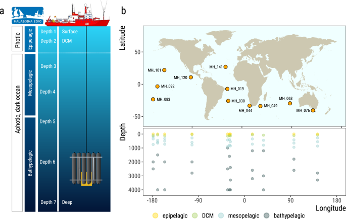
The Malaspina expedition microbial picoplankton vertical profiles. (a) Schematics of a typical vertical profile sampling event. Water samples were collected at seven depths from the surface to the ocean bottom or 4,000 m deep, targeting 3 layers from the photic and dark ocean: epipelagic, including surface and DCM, mesopelagic and bathypelagic. (b) Map showing the sampling stations of the Malaspina Expedition presented in this data set, along the tropical and sub-tropical global Ocean, and the depths from where water was collected for metagenomic sequencing of the 0.2–3 µm plankton size fraction.
-
(ii)
a total of 25.3 Gbp of assembled contigs (332.9 Mbp ± 50.3 per sample, mean ± standard deviation obtained following the bioinformatics workflow depicted in Fig. 2; Supplementary Table 4). A fraction of 67.1% ± 1.8 of the predicted coding DNA sequences (CDS) in the assembled contigs (446,287 ± 63,375) could be assigned to at least one functional category (Fig. 3): 32.7% ± 1.5 to clusters of orthologous groups (COG)16, 63.7% ± 1.6 to protein families (PFAM)17, 28.3% ± 1.8 to Kyoto Encyclopedia of Genes and Genomes (KEGG)18 orthologs (KO), and 1.1% ± 0.1 to carbohydrate-active enzymes (CAZy)19. A fraction of 34.7% ± 1.6 of CDS could not be assigned to a function with the used databases (Supplementary Table 4). Similarly, 41.7% ± 10.7 CDS (187,334 ± 42,691) per sample could not be taxonomically classified further than “root” or were “unclassified” after aligning them to UniRef9020 using the lowest common ancestor approach (LCA).
-
(iii)
a 17.43 million non-redundant CDS database (M-GeneDB-VP). In total 9,967,787 (57.2%) genes in this gene catalog were annotated with PFAM, 3,717,395 (21.3%) with KOs, 5,097,211 (29.3%) with COGs and 169,855 (0.97%) with CAZy, whereas 8,889,665 genes (43.1%) could not be annotated and correspond to the gene novelty of this database.
-
(iv)
functional profiles of each gene grouped by annotation, consisting of the abundance of each CDS/annotation per sample, based on the number of reads of each metagenome mapping back to the M-GeneDB-VP, corrected by gene length and by single-copy universal marker gene abundance (see below).
-
(v)
A 2,672 medium and high-quality Metagenome-Assembled Genomes (MAGs) of bacteria and archaea (Malaspina-VP-MAGs) with their functional and taxonomic annotations, corresponding to microorganisms from 22 bacterial and 5 archaeal phyla.
-
(vi)
taxonomic profiles of picoplankton, based on the 16S mTAG21 analysis of the metagenomes, including 15,046 OTUs (Fig. 4).
-
(vii)
A total of 101,219 viral genomic sequences of at least one kbp identified in the assembled contigs and 3,105 unique viral sequences identified as prophages within the MAGs sequences.

This Malaspina Microbial Vertical Profiles metagenomes dataset (MProfile) resource will be of great interest to the community to tackle ecologically relevant questions on marine microbial ecology –recently it has been used to identify a universal scaling relationship between prokaryotic genome size and ocean temperature22– such as inferring differential functional traits of photic and aphotic bacterial and archaeal genomes through the reconstruction of metagenome assembled genomes (MAGs), as well as serve as a valuable dataset for gene discovery, with interest in biotechnology and other research areas.
Primary sequencing data and Megahit assemblies have been submitted to the European Nucleotide Archive. Derived data such as M-GeneDB-VP, annotations and files for functional and taxonomic profiles, MAG sequences, MAGs descriptive information, MAGs annotation, MAGs coding DNA and protein encoding gene sequences, viral genomic sequences, viral genomic sequences descriptive information and annotation of virus-derived coding DNA sequences have been submitted to the European Bioinformatics Institute BioStudies repository (accession S-BSST105923) to allow further exploration of the functional and taxonomic composition and vertical connectivity of the ocean microbiome.
Methods
Sample collection
A total of 76 water samples were taken during the Malaspina 2010 expedition (http://www.expedicionmalaspina.es) on board the R/V Hespérides from January 4 to July 5, 2011 (Supplementary Table 2), corresponding to 11 different sampling stations (Fig. 1b). Each station was profiled by collecting water from 7 discrete depths (except station MH_120, with 6 depths) from surface (3 m) to the bathypelagic layer, down to 4,000 m (mean maximum depth of each profile 3,491 ± 626 m), including the deep chlorophyll maximum (DCM; Fig. 1b; Supplementary Table 2). Water samples were collected either with a rosette of Niskin bottles (12 L each) on a frame with a CTD sensor or with a large Niskin bottle (30 L) for the surface samples. For every sample, two 6-L replicates were pre-filtered sequentially through 200 µm and 20 µm nylon meshes to remove large plankton, and then through a 47 mm diameter polycarbonate (PC) membrane with a 3 µm pore size (Whatman filter ref: 10418312), and a 47 mm diameter PC membrane with a 0.22 µm pore size (Whatman filter ref: GTTP04700) using a peristaltic pump (Masterflex, EW-7741010) with a flow rate of 50–100 ml min−1. When the filtration rate decreased considerably, filters were replaced. The 0.22 µm filters, including the free-living (FL) prokaryotic community24,25 as well as picoeukaryotes, were packaged in 2-mL cryotubes, flash frozen in liquid nitrogen and stored in a freezer at −80 °C. All collection equipment was decontaminated between samples using ethanol and 0.1% bleach. The time span from bottle closing of the deep sample to filter freezing was approximately 4 h, and except for the time needed to empty the rosette bottles, the water was kept at 4 °C.
DNA extraction
DNA was extracted with the standard phenol-chloroform protocol with slight modifications21,26. Detailed description of the DNA extraction protocol used in our lab have been previously published27. Briefly, the filters were cut in small pieces with sterile razor blades and resuspended in 3 mL of lysis buffer (40 mM EDTA, 50 mM Tris-HCl, 0.75 M sucrose). Samples were incubated at 37 °C for 45 min in lysis buffer (Lysozyme; 1 mg mL−1 final concentration) with gentle agitation. Then, the buffer was supplemented with sodium dodecyl sulfate (SDS, 1% final concentration) and proteinase K (0.2 mg mL−1 final concentration) and the samples were incubated at 55 °C for 60 min under gentle agitation. The lysate was collected and processed with the standard phenol-chloroform extraction procedure: an equal volume of Phenol:CHCl3:IAA (25:24:1, vol:vol:vol) was added to the lysate, mixed and centrifuged 10 min at 3,000 rpm. Then the aqueous phase was recovered and the procedure was repeated. Finally, residual phenol was removed by adding an equal volume of CHCl3:IAA (24:1, vol:vol) to the recovered aqueous phase. The mixture was centrifuged and the aqueous phase was recovered for further purification. The aqueous phase was then concentrated by centrifugation with a Centricon concentrator (Millipore, Amicon Ultra-4 Centrifugal Filter Unit with Ultracel-100 membrane). This step was repeated three times by adding 2 mL of sterile Milli-Q water each time to wash away any impurities that could interfere with the library preparation. The genomic DNA extract was concentrated down to 100 to 200 μL of volume.
Sequencing
An average of 0.6 µg (minimum of 0.25 µg) of extracted DNA was sent and sequenced on the Illumina HiSeq 2000 platform at the Centre Nacional d’Anàlisi Genòmica (CNAG) in Barcelona, Spain. The libraries were sequenced using TruSeq SBS Kit v3-HS (Illumina, Inc), in paired-end mode with a read length of 2 × 101 bp following the manufacturer’s protocol. Images analysis, base calling and quality scoring of the run were processed using the manufacturer’s software Real Time Analysis (RTA 1.13.48, HCS 1.5.15.1) and followed by generation of FASTQ sequence files by CASAVA, yielding a total of 1.66 Tbp (108.1 ± 2.8 million read pairs and 21.8 ± 0.6 Gbp per sample; mean ± standard deviation). Fastq files with the clean reads for all 76 samples are available at ENA under the BioProject accession number PRJEB5245228 (Supplementary Table 1).
Bioinformatics workflow
The bioinformatics workflow applied to this data set is summarized in Fig. 2 and consisted in the following steps:

Bioinformatics workflow for processing metagenomes. Summary of the bioinformatics workflow used to process 76 metagenomes from 11 vertical profiles from the Malaspina Expedition, including seven depths from the surface to the ocean bottom or 4,000 m deep per sample. Processes or analyses are highlighted in green, the tools used in each process are highlighted in purple and selected results of each analysis are shaded in pink.
The quality of raw read pairs was checked with FastQC v0.11.7 (https://www.bioinformatics.babraham.ac.uk/projects/fastqc/), and Illumina TruSeq adapter contamination was removed in Trimmomatic v0.3829 keeping adapter-free read pairs with contiguous quality over 20 and a minimum length of 45 bp with options “ILLUMINACLIP:2:30:10 LEADING:3 SLIDINGWINDOW:4:20 MINLEN:45”. Unpaired reads were discarded for further steps. After trimming, the dataset consisted of a total of 1.15 Tbp, with 81.5 ± 4.6 million clean read pairs and 15.1 ± 1.1 Gbp per sample (Supplementary Table 3).
Clean reads of each sample were assembled in Megahit v1.1.330 with options “--presets meta-large --min-contig-len 500” to produce a total of 25.3 Gbp of metagenomic assemblies (332.9 Mbp ± 50.3, n = 76). The minimum contig size was set to 500 bp following Tara Ocean’s assembly protocol31 to make both datasets more homogeneous. In order to work only with the prokaryotic fraction of the assemblies, contigs were screened with Tiara v1.0.232 with options “--min_len 500 --pr” and those marked as “eukarya” or “organelle” were not taken into account for further analyses. Eukaryotic contigs accounted for 11% of the total assembled basepairs (59.5 Mbp ± 28.3). Prokaryotic contigs were annotated in Prokka v1.14.633 for gene prediction based in Prodigal34 (options -c -m -g 11 -p meta; considering only complete genes), clusters of orthologous groups (COGs)16, Enzyme Commission numbers (EC) and gene product name. Additionally, predicted genes amino acid sequences were annotated for protein families’ domains (PFAM v34)17 using HMMER v3.33 (hmmsearch)35 with option “-E 0.1”, the Kyoto Encyclopedia of Genes and Genomes Orthologs (KEGG KO)18 release v98.0 using KofamScan v1.3.036 and options “–format detail -E 0.01”, and carbohydrate active enzymes (CAZy) using HMMER v3.33 (hmmsearch) against dbCAN v1019.
PFAM hmmsearch results were obtained with very low stringency (E = 0.1). The best hit was awarded for each model that aligned with no overlap to the predicted genes. This means that a single gene might have more than one protein domain annotation. When two or more hits were aligning in the same region, if the overlap was longer than half the length of the smaller alignment, the hit with larger bitscore was kept as the best one for that region.
Similarly, KofamScan (E = 0.01) results were filtered by keeping all hits with scores above the predefined thresholds for individual KOs (marked with an ‘*’), potentially assigning more than one KO to a single predicted gene.
Predicted coding sequences were taxonomically assigned by mapping them to UniRef9020, release 2021_03 from 9 of June 2021, with MMseqs237 development version, commit 13-45111, with the taxonomy workflow options “--max-accept 100 --tax-lineage 1 -e 1E-5 -v 3 -a” and converted to table with mmseqs createtsv. All ranks out of domain, phylum, class, order, family, genus or species were removed from classification and missing fields were marked as “unclassified”. The lowest common ancestor for each sequence was also recorded. Genes from prokaryotic contigs classified as domain Eukarya were further removed from the dataset.
Gene catalog
In order to reduce the redundancy of the predicted gene dataset, we clustered all coding DNA sequences longer than 100 bp to 95% nucleotide sequence similarity and 90% alignment coverage of the shorter sequence in CD-HIT v4.6.138 with cd-hit-est and options “-c 0.95 -G 0 -aS 0.9 -g 1 -r 1 -d 0 -s 0.8”. We used the longest sequence of each cluster as the representative sequence, obtaining a catalog of 17,425,759 non-redundant genes. We refer to this set of coding sequences as the Malaspina Vertical Profiles Gene Database (M-GeneDB-VP)23. Functional and taxonomic annotation of the M-GeneDB-VP genes was inherited from the annotation of representative sequence of each cluster, as described above23.
Functional profiling
Clean reads were back-mapped to the catalog with Bowtie2 v2.4.339 and alignments were filtered with Samtools v1.1540 with option “-F 4” to keep only primary alignments. Reads mapping to catalog genes were counted in htseq-count from HTSeq v2.0.441 with options “--nonunique all --minaqual 0” to build gene profiles per sample. As genes in a catalog are stripped from their genomic context, a read mapping to 2 contiguous genes in a genome would be randomly assigned to just one in the catalog. This option allows counting one read to more than one gene and to get a more inclusive representation of the abundance of each gene of the catalog by mapping it to all features it was assigned to, instead of randomly imputing it to only one. Counts were normalized by gene length in bp and then normalized by the geometric median abundance of 10 universal single-copy phylogenetic marker genes either for COGs (COG0012, COG0016, COG0018, COG0172, COG0215, COG0495, COG0525, COG0533, COG0541, and COG0552) or KOs (K01409, K01869, K01873, K01875, K01883, K01887, K01889, K03106, K03110, K06942) respectively. Normalizing coverage-corrected read counts by the abundance of these marker genes acts as a proxy to the number of gene copies per cell42. Functional profiles for COGs, PFAMs, KOs and CAZymes were calculated by adding up abundance values corresponding to genes annotated as a particular function, both from the gene length normalized table and the single-copy marker gene normalized table23. Functional richness was calculated by converting gene length normalized tables to pseudo-counts (multiplying abundance values by 10,000 and rounding to the next integer) and rarefying to 0.95 times the minimal sample sum with function rtk in R package rtk v0.2.6.143 (Fig. 3).

Prokaryotic functional richness (KO, PFAM, COG, CAZy) of 76 metagenomes grouped by depth layer. Functional richness of the prokaryotic fraction of 76 metagenomes from 11 vertical profiles from the Malaspina Expedition showed by ocean layer: epipelagic excluding the deep chlorophyll maximum (DCM) (from 0 to 200 m deep), DCM, mesopelagic (200 to 1,000 m deep) and bathypelagic (1,000 to 4,000 m deep), for KEGG orthologs (KO), protein families (PFAM), clusters of orthologous groups (COG) and carbohydrate-active enzymes (CAZy). Richness is calculated by converting gene abundances in the gene length normalized abundance tables for each feature to pseudo-counts and rarefying to 0.95 times the minimal sample sum with function rtk in R package rtk v0.2.6.1. Significant differences in richness values between ocean layers are depicted with different letters (Kruskal-Wallis, p < 0.05; Dunn’s post-hoc test with Holm correction for multiple comparisons).

Sample prokaryotic taxonomic composition (richness and sample ordination) based in the analysis of mTAGS (16S rRNA SSU metagenomic fragments). (a) OTU richness based on 16S mTAGs analysis, showed by ocean layer: epipelagic excluding the deep chlorophyll maximum (DCM) (from 0 to 200 m deep), DCM, mesopelagic (200 to 1,000 m deep) and bathypelagic (1,000 to 4,000 m deep). Significant differences in richness values between ocean layers are depicted with different letters (Kruskal-Wallis, p < 0.05; Dunn’s post-hoc test with Holm correction for multiple comparisons). (b) Ordination plot (non-metric multidimensional scaling; Bray-Curtis distance) of 76 metagenomes from 11 vertical profiles based on their community composition (16S mTAG OTUs) colored by ocean layer as described above.
Metagenome assembled genomes
Aiming to obtain high-quality Metagenome Assembled Genomes (MAGs), metagenomes were assembled individually using MetaSPAdes v3.13.044. A Bowtie2 v2.3.4.139 database was built using contigs longer than 2.5 kbp from all metagenomes. Next, post-QC metagenomic reads were queried against the aforementioned database using Bowtie2 in sensitive local mode. Output SAM files were converted to BAM and sorted using Samtools v1.1540. Sorted bam files were then used to calculate the contig abundance summary table using the jgi_summarize_bam_contig_depths script available through the Metabat repository (https://bitbucket.org/berkeleylab/metabat/src/master/). Finally, genome binning was performed for each individual metagenome using Metabat v2.12.145. Completeness and contamination of the generated genome bins was estimated through CheckM v1.1.646. Only bins with at least 50% completeness were kept for subsequent analysis. Among those, bins for which the contamination was estimated to be 5% or higher were subjected to a custom bin decontamination step as follows: first, each contig was assigned taxonomic annotation using CAT v5.2.347, with option “--fraction 0.05”. Next, each contaminated bin was split into multiple sub-bins according to the class level taxonomic classification of each contig within it. The sub-bins were assessed for completeness and contamination as above. Finally, only bins with at least 50% completeness and less than 5% contamination were kept for subsequent analysis. These represent 2,672 medium and high-quality draft genomes according to MIMAG standards48 (Supplementary Table 5, BioStudies accession S-BSST105923). Phylogenomic reconstruction and taxonomic classification of MAGs was carried out through GTDB-tk v1.749 (Supplementary Table 5), and the resulting tree (Fig. 5) was decorated in iTOL50. MAGs were clustered using DRep v3.2.251 into 1,228 non-redundant species clusters. Notably, 94 cluster representatives were obtained through our automated bin refinement method, meaning that without this step these 94 genome representatives would have yielded lower quality MAGs or not be identified in our dataset at all. This draws attention to the potential of automated bin refinement strategies as an efficient way to produce more MAGs and of higher quality, allowing for better characterization of genomic diversity within metagenomes. Taxonomic classification through phylogenomic reconstruction assigned MAGs to 22 bacterial and 5 archaeal phyla, which represented both ubiquitous and abundant taxa from marine ecosystems, such as Alphaproteobacteria, Cyanobacteria, and Thermoproteota, as well as low abundance taxa, such as Eremiobacterota, Margulisbacteria, Myxococcota, and UBP7. Overall, 509 out of 1,228 non-redundant MAGs were assigned to new species, one of which represented a new order within the class Planctomycetes.

Diversity of prokaryotic MAGs from 76 metagenomes from 11 vertical profiles from the Malaspina Expedition based on GTDB-tk phylogenomic reconstruction and taxonomic classification. (a) Phylogenomic tree of Bacterial diversity. (b) Phylogenomic tree of Archaeal diversity. Stacked bar plots display the total number of MAGs obtained from each depth layer. All clades were collapsed at the level of Phylum and branch lengths were omitted to better display the tree topology.
MAG relative abundances and community composition
Relative abundances of MAGs and taxa were calculated as follows. A second Bowtie2 database was built, this time containing only the contigs associated with the set of 1,228 de-replicated medium and high-quality MAGs. Next, post-QC reads from the metagenomes were queried against the MDB using Bowtie2 in sensitive local mode. Output SAM files were converted to BAM and sorted using Samtools. Contig relative abundances were calculated as Reads Per Kilobase per Million total sequences (RPKM). MAG relative abundances, at each metagenome sample, were calculated as the sum of the RPKM values of the contigs according to the MAG to which they belonged. Finally, taxon relative abundances, at each metagenome sample, were calculated as the sum of the RPKM values of the MAGs according to the Phylum (or class for Proteobacteria) to which they were assigned (Fig. 6).

Taxonomic composition across communities from different depth zones, estimated by MAG relative abundances. Bar plots depict the mean relative abundances of MAGs grouped according to phyla (or class for Proteobacteria), across metagenomes grouped according to the depth zone from which metagenomes were obtained. Error bars represent standard deviations.
Taxonomic profiling
Additional taxonomic profiling of the prokaryotic composition was added to the previous MAG community description. MAGs alone don’t use all the available sequencing information and rarer organisms may remain undetected. In order to capture as much taxonomic information of each metagenome and to be able to explore the community composition relationships between depth layers we identified and classified mTAGs, 16S ribosomal RNA gene small subunit (SSU) fragments, directly from the Illumina-sequenced metagenomes21 with mTAGs v1.0.452, profile workflow with options “-ma 1000 -mr 1000”. This protocol is particularly suitable for metagenomes with short reads, as it takes advantage of a degenerated consensus reference database and an exhaustive search strategy, reducing the number of ambiguously mapped sequences that could not be used for classification. Briefly, the mTAGs pipeline extracts reads from the metagenome, which are identified as SSU-rRNA gene sequences by using hidden Markov models, and then maps them to a reference sequence database based on SILVA 13853, pre-clustered at 97% of sequence similarity and with degenerated consensus sequences within each OTU. It then classifies mTAGs conservatively to a taxonomic rank by considering its lowest common ancestor. Finally, it builds taxonomic profiles at different ranks, including the OTU level23. OTUs classified as “class Cyanobacteriia; order Chloroplast” or “family Mitochondria” were removed from the OTU counts table. The OTU count table was rarefied (5,861 reads/sample) using the rrarefy function in the R package vegan v2.5.754 to correct for uneven sequencing depths among samples.
Identification of viral sequences among assembled contigs
VIBRANT v1.2.155 was used to identify viral genomic sequences derived from dsDNA viruses of archaea and bacteria among the assembled contigs. VirSorter255 was applied to identify sequences derived from Nucleo-Cytoplasmic Large DNA Viruses (NCLDV), virophages (Lavidaviridae), and ssDNA viruses. Next, CheckV v0.8.156 was applied to assess the quality (i.e., completeness and host contamination) of the obtained viral genomic sequences. A total of 123,976 viral genomic sequences were identified, among which 302 were considered high-quality (Completeness > = 90%, and contamination = 0%) according to MIUVIG standards57. Computational host predictions were performed using PHIST version ed2a1e658. For the PHIST analysis, only predictions with a maximum e-value of 2.384e-14 were considered, which yields approximately 85% class level prediction accuracy. The collection of 2,672 MAGs was used as a set of putative hosts. Putative hosts were assigned to 9,543 viral genomic sequences23, the most frequent host assignments were to Alphaproteobacteria (3,244 contigs), Gammaproteobacteria (1,826), Marinisomatota (894), Bacteroidota (881) and Actinobacteriota (734).
Annotation of MAGs and viral genomic sequences
Coding DNA Sequences (CDS) derived from MAGs and viral genomic sequences23 were queried against three databases for annotation: (1) UniRef10020 using DIAMOND v2.0.759, (2) KOFam36 using hmmscan in HMMER v3.335, (3) PFAM17 using HMMER’s hmmscan as well. For all searches, only hits that displayed a bitscore ≥50 and e-value ≤ 10−5 were considered as valid hits and included in the annotation tables23.
Data Records
All sequencing products described here, as well as the primary metagenome assemblies, can be found under BioProject accession number PRJEB52452 hosted by the European Nucleotide Archive28. ENA accession numbers for each metagenome sequencing run and for each megahit assembly are provided in Supplementary Tables 1, 4 respectively.
File 1: 17,425,759 non-redundant coding DNA sequences (gene catalog) can be found in MP-GeneDB-VP.fasta.gz23.
File 2: Prokka annotation for each CDS from the gene catalog, plus annotations for PFAM, KEGG-KO, CAZy and lowest common ancestor taxonomy can be found in file MP-GeneDB-VP-annotation-enhanced.tsv.gz23.
File 3: 16S rRNA mTAG-based OTU table of the 76 metagenomes can be found in file mp-mtags.otu.tsv23.
File 4: Counts of reads from each metagenome mapping to the gene catalog can be found in file MP-GeneDB-VP-raw-counts.tbl.gz23.
File 5: Counts of reads from each metagenome mapping to the gene catalog normalized by gene length can be found in file MP-GeneDB-VP-length-norm-counts.tbl.gz23.
File 6: Counts of reads from each metagenome mapping to the gene catalog annotated to COGs, normalized by gene length and 10 universal single copy COGs can be found in file MP-GeneDB-VP-length-norm-scgNorm-counts-cog.tbl.gz23.
File 7: Counts of reads from each metagenome mapping to the gene catalog annotated to KEGG KOs, normalized by gene length and 10 universal single copy KOs can be found in file MP-GeneDB-VP-length-norm-scgNorm-counts-ko.tbl.gz23.
File 8. Counts of reads from each metagenome mapping to the gene catalog normalized by gene length and aggregated per COG can be found in file MP-GeneDB-VP-length-norm-cog.tbl.gz23.
File 9. Counts of reads from each metagenome mapping to the gene catalog normalized by gene length and aggregated per KO can be found in file MP-GeneDB-VP-length-norm-ko.tbl.gz23.
File 10. Counts of reads from each metagenome mapping to the gene catalog normalized by gene length and aggregated per PFAM can be found in file MP-GeneDB-VP-length-norm-pfam.tbl.gz23.
File 11. Counts of reads from each metagenome mapping to the gene catalog normalized by gene length and aggregated per CAZy can be found in file MP-GeneDB-VP-length-norm-cazy.tbl.gz23.
File 12: fasta sequences for the 2,672 MAGs with estimated genome completeness above 50% and contamination below 5% can be found at file Malaspina-VP-MAGs.tar.gz23.
File 13. Functional annotation of each MAG can be found in file Malaspina-VP-MAGs_CDS-annotation.tsv.gz23.
File 14. Amino acid sequences of predicted genes in the MAGs sequences can be found in file Malaspina-VP-MAGs_CDS.faa.gz23.
File 15: Nucleotide sequences of predicted genes in the MAGs sequences can be found in file Malaspina-VP-MAGs_CDS.fna.gz23.
File 16: Viral genomic sequences can be found in file Malaspina_Profiles_Viruses_Genomic_Sequences.fasta.gz23.
File 17: Descriptive information on the viral genomic sequences can be found in file Malaspina_Profiles_Viruses_Genomic_Info.tsv23.
File 18: Virus-derived coding DNA sequences can be found in file Malaspina_Profiles_Viruses_CDS_Sequences.fna.gz23.
File 19: Information of the annotation of the protein encoding genes predicted in the viral genomic sequences can be found in file Malaspina_Profiles_Viruses_PEG_Annotation_Info.tsv23.
Underway and meteorological data measured on board R/V Hesperides for all 7 legs of the Malaspina Expedition 2010 on board R/V Hespérides are available from the Marine Technology Unit (UTM, CSIC)60,61,62,63,64,65,66.
Technical Validation
Extracted DNA was quantified using a Nanodrop ND-1000 spectrophotometer (NanoDrop Technologies Inc, Wilmington, DE, USA) and the Quant_iT dsDNA HS Assay Kit with a Qubit fluorometer (Life Technologies, Paisley, UK).
The sequencing error rate was calculated by the sequencing center using PhiX147 phage DNA spikes (0.4% ± 0.1).
Usage Notes
The metagenomic sequence files deposited at the ENA described here are raw sequences and have not been pre-processed in any way. Before using this data set for re-analysis it is advised to screen sequencing files with current quality-control tools such as the ones used here.
Code availability
All the software used to process the data set presented here is publicly available and distributed by their developers. All versions have been specified in the main text, along with the options used when departing from defaults. Custom scripts used in intermediate or summarizing steps are available at https://gitlab.com/malaspina-public/picoplankton-vertical-profiles.
Code for bin decontamination step can be found at https://github.com/felipehcoutinho/QueroBins.
References
Bar-On, Y. M., Phillips, R. & Milo, R. The biomass distribution on Earth. Proc. Natl. Acad. Sci. 115, 6506–6511 (2018).
Cho, B. C. & Azam, F. Major role of bacteria in biogeochemical fluxes in the ocean’s interior. Nature 332, 441–443 (1988).
Yooseph, S. et al. The Sorcerer II global ocean sampling expedition: Expanding the universe of protein families. PLoS Biol. 5, e16 (2007).
Karsenti, E. et al. A holistic approach to marine Eco-systems biology. PLoS Biol. 9, e1001177 (2011).
Duarte, C. M. Seafaring in the 21St Century: The Malaspina 2010 Circumnavigation Expedition. Limnol. Oceanogr. Bull. 24, 11–14 (2015).
Biller, S. J. et al. Marine microbial metagenomes sampled across space and time. Sci. Data 5, 180176 (2018).
Larkin, A. A. et al. High spatial resolution global ocean metagenomes from Bio-GO-SHIP repeat hydrography transects. Sci Data 8, 107 (2021).
Karl, D. M. & Church, M. J. Microbial oceanography and the Hawaii Ocean Time-series programme. Nat. Rev. Microbiol. 12, 699–713 (2014).
Ruiz‐González, C. et al. Higher contribution of globally rare bacterial taxa reflects environmental transitions across the surface ocean. Mol. Ecol. 28, 1930–1945 (2019).
Villarino, E. et al. Large-scale ocean connectivity and planktonic body size. Nat. Commun. 9, 142 (2018).
Salazar, G. et al. Global diversity and biogeography of deep-sea pelagic prokaryotes. ISME J. 10, 596–608 (2016).
Pernice, M. C. et al. Global abundance of planktonic heterotrophic protists in the deep ocean. ISME J. 9, 782–792 (2015).
Salazar, G. et al. Particle-association lifestyle is a phylogenetically conserved trait in bathypelagic prokaryotes. Mol. Ecol. 24, 5692–5706 (2015).
Acinas, S. G. et al. Deep ocean metagenomes provide insight into the metabolic architecture of bathypelagic microbial communities. Commun. Biol. 4, 1–15 (2021).
Coutinho, F. H. et al. Water mass age structures the auxiliary metabolic gene content of free-living and particle-attached deep ocean viral communities. Microbiome 11, 118 (2023).
Galperin, M. Y., Makarova, K. S., Wolf, Y. I. & Koonin, E. V. Expanded Microbial genome coverage and improved protein family annotation in the COG database. Nucleic Acids Res. 43, D261–D269 (2015).
El-Gebali, S. et al. The Pfam protein families database in 2019. Nucleic Acids Res. 47, D427–D432 (2019).
Kanehisa, M. & Goto, S. KEGG: Kyoto Encyclopedia of Genes and Genomes. Nucleic Acids Res. 28, 27–30 (2000).
Yin, Y. et al. dbCAN: a web resource for automated carbohydrate-active enzyme annotation. Nucleic Acids Res. 40, W445–51 (2012).
Suzek, B. E., Wang, Y., Huang, H., McGarvey, P. B. & Wu, C. H. UniRef clusters: A comprehensive and scalable alternative for improving sequence similarity searches. Bioinformatics 31, 926–932 (2015).
Logares, R. et al. Metagenomic 16S rDNA Illumina tags are a powerful alternative to amplicon sequencing to explore diversity and structure of microbial communities. Environ. Microbiol. 16, 2659–2671 (2013).
Ngugi, D. K. et al. Abiotic selection of microbial genome size in the global ocean. Nat. Commun. 14, 1384 (2023).
Sánchez, P., Acinas, S. G. & Gasol, J. M. Supplemental data for 76 marine picoplankton metagenomes from eleven vertical profiles obtained by the Malaspina Expedition in the tropical and sub-tropical oceans. BioStudies database https://identifiers.org/biostudies:S-BSST1059 (2023).
Crump, B. C., Armbrust, E. V. & Baross, J. A. Phylogenetic Analysis of Particle-Attached and Free-Living Bacterial Communities in the Columbia River, Its Estuary, and the Adjacent Coastal Ocean. Appl. Environ. Microbiol. 65, 3192–3204 (1999).
Ghiglione, J. F., Conan, P. & Pujo-Pay, M. Diversity of total and active free-living vs. particle-attached bacteria in the euphotic zone of the NW Mediterranean Sea. FEMS Microbiol. Lett. 299, 9–21 (2009).
Mestre, M. et al. Sinking particles promote vertical connectivity in the ocean microbiome. Proc. Natl. Acad. Sci. 115, E6799–E6807 (2018).
Salazar, G. et al. Global diversity and biogeography of deep-sea pelagic prokaryotes. ISME J. 10, 1–13 (2015).
ENA European Nucleotide Archive. https://identifiers.org/ena.embl:PRJEB52452 (2023).
Bolger, A. M., Lohse, M. & Usadel, B. Trimmomatic: a flexible trimmer for Illumina sequence data. Bioinforma. Oxf. Engl. 30, 2114–2120 (2014).
Li, D. et al. MEGAHIT v1.0: A fast and scalable metagenome assembler driven by advanced methodologies and community practices. Methods 102, 3–11 (2016).
Sunagawa, S. et al. Structure and function of the global ocean microbiome. Science 348, 1261359 (2015).
Karlicki, M., Antonowicz, S. & Karnkowska, A. Tiara: deep learning-based classification system for eukaryotic sequences. Bioinformatics 38, 344–350 (2021).
Seemann, T. Prokka: Rapid prokaryotic genome annotation. Bioinformatics 30, 2068–2069 (2014).
Hyatt, D. et al. Prodigal: prokaryotic gene recognition and translation initiation site identification. BMC Bioinformatics 11, 119 (2010).
Eddy, S. R. Accelerated profile HMM searches. PLoS Comput. Biol. 7(e1002195), 1–16 (2011).
Aramaki, T. et al. KofamKOALA: KEGG ortholog assignment based on profile HMM and adaptive score threshold. Bioinformatics 36, 2251–2252 (2019).
Steinegger, M. & Söding, J. MMseqs. 2 enables sensitive protein sequence searching for the analysis of massive data sets. Nat. Biotechnol. 35, 1026–1028 (2017).
Li, W. & Godzik, A. Cd-hit: A fast program for clustering and comparing large sets of protein or nucleotide sequences. Bioinformatics 22, 1658–1659 (2006).
Langmead, B. & Salzberg, S. L. Fast gapped-read alignment with Bowtie 2. Nat. Methods 9, 357–359 (2012).
Li, H. et al. The Sequence Alignment/Map format and SAMtools. Bioinformatics 25, 2078–2079 (2009).
Anders, S., Pyl, P. T. & Huber, W. HTSeq–a Python framework to work with high-throughput sequencing data. Bioinforma. Oxf. Engl. 31, 166–169 (2015).
Salazar, G. et al. Gene Expression Changes and Community Turnover Differentially Shape the Global Ocean Metatranscriptome. Cell 179, 1068–1083 (2019).
Saary, P., Forslund, K., Bork, P. & Hildebrand, F. RTK: efficient rarefaction analysis of large datasets. Bioinformatics 33, 2594–2595 (2017).
Nurk, S., Meleshko, D., Korobeynikov, A. & Pevzner, P. A. metaSPAdes: a new versatile metagenomic assembler. Genome Res. 27, 824–834 (2017).
Kang, D. D., Froula, J., Egan, R. & Wang, Z. MetaBAT, an efficient tool for accurately reconstructing single genomes from complex microbial communities. PeerJ 3, e1165 (2015).
Parks, D. H., Imelfort, M., Skennerton, C. T., Hugenholtz, P. & Tyson, G. W. CheckM: assessing the quality of microbial genomes recovered from isolates, single cells, and metagenomes. Genome Res. 25, 1043–1055 (2015).
von Meijenfeldt, F. A. B., Arkhipova, K., Cambuy, D. D., Coutinho, F. H. & Dutilh, B. E. Robust taxonomic classification of uncharted microbial sequences and bins with CAT and BAT. Genome Biol. 20, 217 (2019).
Bowers, R. M. et al. Minimum information about a single amplified genome (MISAG) and a metagenome-assembled genome (MIMAG) of bacteria and archaea. Nat. Biotechnol. 35, 725–731 (2017).
Chaumeil, P.-A., Mussig, A. J., Hugenholtz, P. & Parks, D. H. GTDB-Tk: a toolkit to classify genomes with the Genome Taxonomy Database. Bioinformatics 36, 1925–1927 (2019).
Letunic, I. & Bork, P. Interactive Tree Of Life (iTOL) v4: recent updates and new developments. Nucleic Acids Res. 47, W256–W259 (2019).
Olm, M. R., Brown, C. T., Brooks, B. & Banfield, J. F. dRep: a tool for fast and accurate genomic comparisons that enables improved genome recovery from metagenomes through de-replication. ISME J. 11, 2864–2868 (2017).
Salazar, G., Ruscheweyh, H.-J., Hildebrand, F., Acinas, S. G. & Sunagawa, S. mTAGs: taxonomic profiling using degenerate consensus reference sequences of ribosomal RNA genes. Bioinformatics 38, 270–272 (2022).
Quast, C. et al. The SILVA ribosomal RNA gene database project: improved data processing and web-based tools. Nucleic Acids Res. 41, D590–D596 (2013).
Dixon, P. VEGAN, a package of R functions for community ecology. J. Veg. Sci. 14, 927–930 (2003).
Kieft, K., Zhou, Z. & Anantharaman, K. VIBRANT: automated recovery, annotation and curation of microbial viruses, and evaluation of viral community function from genomic sequences. Microbiome 8, 90 (2020).
Nayfach, S. et al. CheckV assesses the quality and completeness of metagenome-assembled viral genomes. Nat. Biotechnol. 39, 578–585 (2021).
Roux, S. et al. Minimum Information about an Uncultivated Virus Genome (MIUViG). Nat. Biotechnol. 37, 29–37 (2019).
Zielezinski, A., Deorowicz, S. & Gudyś, A. PHIST: fast and accurate prediction of prokaryotic hosts from metagenomic viral sequences. Bioinformatics 38, 1447–1449 (2022).
Buchfink, B., Xie, C. & Huson, D. H. Fast and sensitive protein alignment using DIAMOND. Nat. Methods 12, 59–60 (2014).
Duarte, C. M., UTM-CSIC. MALASPINA_LEG1 Cruise, RV Hespérides. https://doi.org/10.20351/29HE20101215 (2010).
Duarte, C. M., UTM-CSIC. MALASPINA_LEG2 Cruise, RV Hespérides. https://doi.org/10.20351/29HE20110117 (2011).
Duarte, C. M., UTM-CSIC. MALASPINA_LEG3 Cruise, RV Hespérides. https://doi.org/10.20351/29HE20110211 (2011).
Duarte, C. M. & UTM-CSIC MALASPINA_LEG4 Cruise, RV Hespérides. https://doi.org/10.20351/29HE20110317 (2011).
Duarte, C. M., UTM-CSIC. MALASPINA_LEG5 Cruise, RV Hespérides. https://doi.org/10.20351/29HE20110416 (2011).
Duarte, C. M., UTM-CSIC. MALASPINA_LEG6 Cruise, RV Hespérides. https://doi.org/10.20351/29HE20110513 (2011).
Duarte, C. M., UTM-CSIC. MALASPINA_LEG7 Cruise, RV Hespérides. https://doi.org/10.20351/29HE20110619 (2011).
Acknowledgements
We thank the R/V Hespérides captain and crew, the chief scientists in the Malaspina expedition legs, and all project participants for their help in making this project possible. This work was funded by the Spanish Ministry of Economy and Competitiveness (MINECO) through the Consolider-Ingenio program (Malaspina 2010 Expedition, ref. CSD2008-00077). The sequencing of 76 metagenomes from 11 vertical profiles was funded by project Malaspinomics and Malaspina-analytics (CTM2011-15461-E) awarded to C.M.D. by the Spanish Ministry of Economy and Competitiveness. Additional funding was provided by the project MAGGY (CTM2017-87736-R) to S.G.A. from the Spanish Ministry of Economy and Competitiveness, Grup de Recerca 2017SGR/ 1568 from Generalitat de Catalunya, and King Abdullah University of Science and Technology (KAUST) under contract OSR #3362. The ICM researchers have had the institutional support of the “Severo Ochoa Centre of Excellence” accreditation (CEX2019-000928-S) funded by AEI10.13039/501100011033. R.R-M. thanks CeBiB FB0001 support. High-Performance computing analyses were run at the Marine Bioinformatics Core facility (MARBITS, https://marbits.icm.csic.es) of the Institut de Ciències del Mar (ICM-CSIC), Barcelona Supercomputing Center (Grant BCV-20132-0001), KAUST’s Ibex HPC and Galicia Supercomputing Center (CESGA).
Author information
Authors and Affiliations
Contributions
P.S. analyzed the data, wrote the code, and wrote the manuscript. F.H.C. analyzed the data, wrote the code, and wrote the manuscript. E.M.L.G. and X.L.A. analyzed the viral data. M.S., M.C.P., R.R-M., G.S. and F.M.C. extracted DNA. M.C.P., G.S., F.M.C., M.M.S. and D.V. participated in the sampling operations. G.S. and F.M.C. contributed to the data analysis. S.P, M.S. and P.S. curated the metadata and defined the biosamples. S.A. contributed funding. T.G. contributed funding. C.M.D. was the chief coordinator of the Malaspina Expedition and contributed funding and computational assistance. S.G.A. defined sampling protocols, coordinated the microbial -omics analyses and contributed funding. J.M.G. coordinated the microbial diversity and ecosystem function area of the Malaspina Expedition and contributed funding. All authors contributed to the final version of the manuscript.
Corresponding authors
Ethics declarations
Competing interests
The authors declare no competing interests.
Additional information
Publisher’s note Springer Nature remains neutral with regard to jurisdictional claims in published maps and institutional affiliations.
Supplementary information
Rights and permissions
Open Access This article is licensed under a Creative Commons Attribution 4.0 International License, which permits use, sharing, adaptation, distribution and reproduction in any medium or format, as long as you give appropriate credit to the original author(s) and the source, provide a link to the Creative Commons licence, and indicate if changes were made. The images or other third party material in this article are included in the article’s Creative Commons licence, unless indicated otherwise in a credit line to the material. If material is not included in the article’s Creative Commons licence and your intended use is not permitted by statutory regulation or exceeds the permitted use, you will need to obtain permission directly from the copyright holder. To view a copy of this licence, visit http://creativecommons.org/licenses/by/4.0/.
About this article

Cite this article
Sánchez, P., Coutinho, F.H., Sebastián, M. et al. Marine picoplankton metagenomes and MAGs from eleven vertical profiles obtained by the Malaspina Expedition. Sci Data 11, 154 (2024). https://doi.org/10.1038/s41597-024-02974-1
Received:
Accepted:
Published:
DOI: https://doi.org/10.1038/s41597-024-02974-1
