
Abstract
Machine-learning interatomic potentials (MLIPs) offer a powerful avenue for simulations beyond length and timescales of ab initio methods. Their development for investigation of mechanical properties and fracture, however, is far from trivial since extended defects—governing plasticity and crack nucleation in most materials—are too large to be included in the training set. Using TiB2 as a model ceramic material, we propose a training strategy for MLIPs suitable to simulate mechanical response of monocrystals until failure. Our MLIP accurately reproduces ab initio stresses and fracture mechanisms during room-temperature uniaxial tensile deformation of TiB2 at the atomic scale ( ≈ 103 atoms). More realistic tensile tests (low strain rate, Poisson’s contraction) at the nanoscale ( ≈ 104–106 atoms) require MLIP up-fitting, i.e., learning from additional ab initio configurations. Consequently, we elucidate trends in theoretical strength, toughness, and crack initiation patterns under different loading directions. As our MLIP is specifically trained to modelling tensile deformation, we discuss its limitations for description of different loading conditions and lattice structures with various Ti/B stoichiometries. Finally, we show that our MLIP training procedure is applicable to diverse ceramic systems. This is demonstrated by developing MLIPs which are subsequently validated by simulations of uniaxial strain and fracture in TaB2, WB2, ReB2, TiN, and Ti2AlB2.
Introduction
Simulations of materials’ mechanical response—including (i) intrinsic strength and toughness, (ii) nucleation of extended defects (e.g., dislocations, stacking faults, cracks) and their implications for (iii) plasticity and fracture mechanisms —require length and time scales beyond limits of ab initio methods ( ≈ 103 atoms, ≪ ns)1,2,3,4. The go-to approach in most cases would be classical Molecular Dynamics (MD), allowing to access atomistic pathways for deformation and fracture in nanoscale systems ( ≈ 106 atoms) and “realistic” operation conditions (e.g., ultra-high temperatures, times up to μs). However, a severe problem of MD is that the necessary interatomic potentials do not exist for most engineering materials or are limited in accuracy and transferability with respect to temperatures, phases, and defective structures (see e.g., refs. 5,6,7).
A powerful avenue for MD simulations on multiple time and length scales with near ab initio accuracy is the application of machine learning interatomic potentials8,9 (MLIPs), in case of no ambiguity just “potentials”). MLIPs learn the atomic energy (or other atomic properties like forces) from a descriptor that characterizes local atomic environments in an ab initio training set10. Compared to conventional ab initio calculations, MD with MLIPs can achieve a speed up of as much as 5 orders of magnitude11,12. Previous studies showed examples of MLIPs’ transferability with respect to defects (e.g., grain boundaries13, dislocation structures14,15) and phases16,17 (e.g., Ni-Mo phase diagram illustrating superior performance of a MLIP over a classical potential18). Recently, Tasnádi et al.19 have demonstrated high accuracy of MLIP-predicted elastic constants for TiAlN ceramics, hence, have set the stage for MLIP development beyond linear elastic regime.
Based on the parametrization of local structural properties, MLIPs can be fitted employing different formalisms: spectral neighbor analysis potentials (SNAP)20, neural networks potentials (NNP)21, Gaussian approximation potentials (GAP)22, moment tensor potentials (MTP)23, linearized interatomic potentials24, or atom cluster expansion (ACE) potentials10. Benchmarks for some of these parametrizations have been published in the case of carbon25 or graphene26, but are missing for chemically complex materials.
Fundamental challenges related to MLIP developments include (i) efficient training dataset generation, (ii) training strategies for simulations beyond length scales feasible for ab initio methods, and (iii) assessing the MLIPs’ reliability over different length scales. Point (ii) closely relates to successively improving the MLIP’s predictive power by up-fitting/active learning27. Here an important concept is the extrapolation/Maxvol grade (γ28) expressing the extent of MLIP’s extrapolation on any structure containing given chemical elements (irrespective of the phase and stoichiometry). Readily available in current ACE and MTP implementations29,30,31, γ allows selecting sufficiently “new” environments to expand the training set. Besides γ, other methods used for selecting configurations are stratified sampling or random selection (for detailed discussion of pros and cons see refs. 32,33,34,35). Besides identifying new environments, γ can serve to indicate the MLIP’s reliability during MD simulations. This is particularly advantageous at scales where the direct validation by ab initio calculations is not possible.
Our work pursues the development of MLIPs suitable to simulate atomic-to-nanoscale deformation of ceramics, providing both methodological and materials science discussion. The model material, TiB2, is a widely studied system, representative of ultra-high temperature ceramics (UHTCs). Exhibiting high hardness and resistance to corrosion, abrasive and erosive wear36,37, UHTCs are suitable to protect tools and machining components under extreme operation conditions38,39,40,41. TiB2, which crystallizes in the AlB2-type phase42,43,44 (α, P6/mmm), exemplifies outstanding mechanical properties45,46 of UTHCs. It exhibits high hardness of 41–53 GPa45,47,48, has a melting point of 3500 K49 and mature synthesis technologies50,51. Insights into mechanical behaviour of TiB2 and other diborides have been offered by ab initio calculations52,53,54 and recently also by molecular dynamics with classical empirical potentials (TiB255,56, ZrB257, HfB258). To date, however, no MLIP capable of predicting mechanical response of UTHCs until fracture has been reported.
Using the MTP formalism, we propose a general training strategy for development of MLIPs targeted to model tensile deformation and fracture of single-crystal ceramics at finite temperatures. The extrapolation grade, γ, is exploited to iteratively improve our MLIP and also as a mean of validation. Specifically, γ values calculated during MD tensile tests are discussed alongside with statistical errors of relevant physical observables, such as time-averaged stresses derived from equivalent ab initio molecular dynamics (AIMD) simulations. The newly-developed MLIP allows to describe tensile deformation in TiB2 supercells with ≈ 103–106 atoms, thus also providing a basis for analyzing size effects on mechanical properties and fracture patterns. Furthermore, we test transferability of our MLIP to other loading conditions and phases, as well as applicability of our general training strategy to other ceramics, exemplified by TaB2, WB2, ReB2, TiN, and Ti2AlB2.
Results and discussion
We aim to develop MLIPs targeted to simulations of tensile deformation in TiB2. Although the mechanical properties of ceramics are typically assessed by nanoindenation, microcantilever bending, or micropillar compression experiments, MD simulations of tensile loading can be directly compared to results of ab initio calculations. We simulate deformation along low-index [0001], [10\(\overline{1}\)0], and [\(\overline{1}2\overline{1}0\)] directions that are parallel or normal to the typical growth direction of hexagonal transition metal diborides36 and have been considered in previous ab initio studies of surface energies and mechanical properties54.
Training procedure and fitting initial MLIPs
Our general training procedure is described below (Procedure 1) and schematically depicted in Fig. 1a (for further details, see the Methods). Throughout this work, training configurations (i.e., structures labelled by ab initio total energies, forces acting on each ion, and six stress tensor components) are generated by finite-temperature AIMD calculations. To avoid over-representation, a training set is initialized by a small fraction of randomly selected AIMD snapshots and iteratively expanded using the concept of the extrapolation grade28, γ.

Schematic visualization of a our general training procedure (Procedure 1, Section Training procedure and fitting initial MLIPs), and b up-fitting (Section MLIPs’validation against atomic scale tensile tests and MLIPs’ up-fitting for nanoscale tensile tests), both applicable to any MLIP formalism with the extrapolation/Maxvol grade (γ) quantification, particularly MTP (used in this work) and ACE. c An overview of the here-developed MLIPs: MLIP-[0001], MLIP-[10\(\overline{1}0\)], MLIP-[\(\overline{1}2\overline{1}0\)] (applicable for atomic scale tensile loading, Sections Training procedure and fitting initial MLIPs and MLIPs’validation against atomic scale tensile tests); MLIP-[1], MLIP-[2], MLIP-[3] (intermediate MLIPs produced by up-fitting, Section MLIPs’ up-fitting for nanoscale tensile tests); and MLIP-[4] (applicable for both atomic and nanoscale tensile loading, Section MLIPs’ up-fitting for nanoscale tensile tests--Otherloading conditions and MLIP’s transferability). Details of the training datasets are given in the corresponding sections and additionally summarized in the Methods under “Development of machine-learning interatomic potentials”. both.
The extrapolation grade γ ∈ R+ (see equations 9–1 in ref. 28) expresses the degree of extrapolation when MLIP predicts atomic properties of a certain configuration. Specifically, γ ≤ 1 means interpolation and γ > 1 extrapolation. Hence, the higher the γ, the larger is the uncertainty on predicted energies, forces, and stresses28. In practice, one sets an extrapolation threshold (γthr). Configurations with γ > γthr are added to the training set to improve transferability of the potential. Procedure 1 uses γthr = 2, motivated by our tests (In particular, during each iteration (i) in the step (4) of Procedure 1, the maximum γ is correlated with errors of energies, forces and stresses (quantified via common regression model evaluation metrics, MAE, RMSE, R2, see e.g., ref. 59) for the TSi (fitting errors) and the VS (validation errors). With γthr = 2, we are limited mainly by the accuracy of the underlying ab initio training data.) as well as by previous work by the MTP developers60 and by one of us12 showing that such value corresponds to accurate extrapolation60 (near-interpolation12).
Procedure 1
MLIP training
(1) Generate a pool of AIMD configurations.
(2) Divide the pool into an initial training set (TS0), a learning set (LS), and a validation set (VS) by randomly selecting 0.5%, 79.5%, and 20% of non-overlapping configurations.
(3) Fit an initial MLIP (MLIP0, trained on TS0). If γ of all configurations in the LS and VS is below γthr = 2, exit. Else, build TS1 by adding maximum 10% of configurations from the LS to TS0, selected by the Maxvol algorithm28 based on their extrapolation grade. Fit a new MLIP (MLIP1, trained on TS1).
(4) While γ of all configurations in the LS and VS is above γthr = 2, build TSi by adding maximum 10% of configurations from the LS to TSi−1, selected by the Maxvol algorithm based on their extrapolation grade. Fit a new MLIP (MLIPi, trained on TSi).
Employing Procedure 1 and the MTP formalism, we fit three MLIPs: MLIP-[0001], MLIP-[10\(\overline{1}0\)], and MLIP-[\(\overline{1}2\overline{1}0\)]. The training uses snapshots from room-temperature AIMD simulations for a 720-atom TiB2 supercell, uniaxially elongated in the [0001], \([10\overline{1}0]\), and \([\overline{1}2\overline{1}0]\) crystallographic direction, respectively, with a strain step of 2% (for details of AIMD simulations, see the Methods). The entire pool of AIMD data consists of ≈ 120, 000 configurations, where each loading condition ([0001], \([10\overline{1}0]\), and \([\overline{1}2\overline{1}0]\)) represents ≈ 1/3.
The final training sets (the last TSi in the step (4) of Procedure 1) of MLIP-[0001], MLIP-[10\(\overline{1}0\)], and MLIP-[\(\overline{1}2\overline{1}0\)] contain 181, 155, and 180 configurations, respectively. The fitting and validation errors, quantified through the residual mean square error (RMSE59), of total energies, forces, and stresses do not exceed 2.6 meV atom−1, 0.11 eV Å−1, and 0.30 GPa, respectively. As follows from Procedure 1, γ < γthr = 2 for all configurations in the learning set.
MLIPs’ validation against atomic scale tensile tests
Following evaluation of the fitting and validation errors (Section Training procedure and fitting initial MLIPs), further validation steps consist in using the above developed MLIPs to run MD simulations (ML-MD) of TiB2 subject to tensile deformation.
During ML-MD, the MLIP’s reliability is assessed via:
-
(i)
Comparison with AIMD predictions of physical, mechanical properties, and fracture mechanisms. In particular, we monitor time-averaged stresses, theoretical strength and toughness, and cleavage on different crystallographic planes.
-
(ii)
The extrapolation grade. At each ML-MD time step, we calculate γ of the corresponding configuration. Values exceeding reliable extrapolation signalise that the MLIP requires up-fitting (i.e., expanding the TS by additional configurations and going back to step (4) of Procedure 1; see Fig. 1b, c).
As suggested by MTP developers60, we consider γreliable ≤ 10 as reliable extrapolation. Such choice allows us to develop MLIPs with accuracy similar to the underlying ab initio training set.
Figure 2 a depicts stress/strain curves derived from room-temperature AIMD and ML-MD tensile tests, in which TiB2 supercell ( ≈ 103 atoms, ≈ 1. 53 nm3) is loaded in the \([0001],[10\overline{1}0]\), and \([\overline{1}2\overline{1}0]\) direction, respectively. Each deformation is simulated with a MLIP trained to the respective loading condition. Excellent quantitative agreement between AIMD and ML-MD results indicates reliability of our MLIPs. Specifically, time-averaged stresses in ML-MD differ from AIMD values by 0.07–1.94 GPa, yielding statistical errors RMSE ≈ 1.02 GPa, R2 ≈ 0.9997. Stresses normal to the loaded direction—not vanishing due to the omission of Poisson’s effect in both AIMD and ML-MD simulations—are also used for assessing MLIPs’ reliability. After fracture, the [0001] stress component recorded in AIMD does not drop to zero. The effect is due to long-range electrostatic effects, which are absent in ML-MD. The extrapolation grade during all ML-MD simulations remains low (γ ≤ 5 < γreliable), thus suggesting reliable extrapolation.

a Comparison of AIMD (dash-dotted line) and ML-MD (solid line) stress/strain curves for TiB2 subject to \([0001],[10\overline{1}0]\), and \([\overline{1}2\overline{1}0]\) tensile deformation at 300 K, using a 720-atom supercell with dimensions of ≈ (1.52 × 1.58 × 2.57) nm3. Only the stress component in the loaded direction is plotted. b, c Snapshots of the fracture point in AIMD (b-1, b-2, b-3) and ML-MD (c-1, c-2, c-3). d Illustration of fracture surfaces (see also ref. 100).
The calculated stress/strain curves allow us to evaluate TiB2’s theoretical tensile strength and toughness along different crystal directions. We report results of the ultimate tensile strength, which corresponds to the global stress maximum during the tensile test61. We define the tensile toughness as the integrated stress/strain area. The property describes the ability of an initially defect-free material at absorbing mechanical energy until failure.
The theoretical tensile strengths of TiB2 obtained by ML-MD are 63.7, 55.0, and 52.7 GPa for the \([\overline{1}2\overline{1}0],[10\overline{1}0]\), and [0001] directions, respectively. These differ from AIMD values by maximum 0.8 GPa (0.99%). The ML-MD predicted toughness along \([\overline{1}2\overline{1}0],[10\overline{1}0]\), and [0001] reaches 4.3, 3.1, and 4.3 GPa, respectively, differing from AIMD values by maximum 0.029 GPa (0.67%). Note, however, that theoretical tensile strength and toughness are affected by the supercell size. Strength and toughness values saturate over nm lengthscales (see following sections).
AIMD and ML-MD tensile-testing of TiB2 reveal very similar fracture mechanisms (Fig. 2b–c). Specifically, the fracture surface formed during [0001] deformation almost perfectly aligns with (0001) basal planes (Fig. 2(b-1),(c-1),d). Tensile loading along the\([10\overline{1}0]\) direction opens a void diagonally across Ti/B2 layers (Fig. 2(b-2),(c-2)). The fracture surface is parallel to the second order pyramidal planes of the \(\{11\overline{2}2\}\) family (Fig. 2d). For the \([\overline{1}2\overline{1}0]\) loading condition, fracture planes are approximately parallel to the \(\{10\overline{1}0\}\) prismatic planes (Fig. 2(b-3),(c-3),d). The TiB2 fracture planes predicted in our simulations are consistent with experimentally-characterized slip planes in single-crystal TiB250,62.
MLIPs’ up-fitting for nanoscale tensile tests
As discussed in the previous section, MLIP-[0001], MLIP-[10\(\overline{1}0\)], and MLIP-[\(\overline{1}2\overline{1}0\)] provide reliable description of TiB2’s response to uniaxial tensile loading at the atomic scale. This is indicated by low extrapolation grades (γ ≤ 5 < γreliable) as well as stress/strain curves and fracture mechanisms in agreement with AIMD results.
As a next step, we carry out tensile tests at the nanoscale. Methodological differences between atomic and nanoscale simulations are listed below.
-
Atomic scale tensile tests (presented in the previous section) employ 720-atom supercells with dimensions of ≈ (1.5 × 1.6 × 2.6) nm3. Strain is incremented at steps of 2% with fixed lattice vectors normal to the loaded direction.
-
Nanoscale tensile tests employ supercells with four different sizes: S1 (12,960 at.), S2 (141,120 at.), S3 (230,400 at.), and S4 (432,000 at.), where S1 ≈ 53 nm3 and S4 ≈ 153 nm3. These simulations impose a continuous and homogeneous increase in strain (rate 50 Å s−1) and account for Poisson’s contraction.
Employing MLIP-[0001], MLIP-[10\(\overline{1}0\)], and MLIP-[\(\overline{1}2\overline{1}0\)] for room-temperature nanoscale tensile tests results in unphysical dynamics (losing atoms) and rapidly increasing extrapolation grades (γ ≫ 103 ≫ γreliable) when approaching the fracture point. This indicates that deformation is controlled by formation of extended crystallographic defects, which are absent in atomic scale simulations. Thus, to enable a description of TiB2’s fracture at the nanoscale, our MLIPs require up-fitting (Fig. 1b). Generally, this is a non-trivial task63,64, since structures causing large γ cannot be directly treated by ab initio calculations.
Below, we describe up-fitting steps leading to MLIP-[4] (schematically depicted in Fig. 1c). We shall see that MLIP-[4] enables reliable simulations of TiB2 tensile deformation at the nanoscale.
-
We produce MLIP-[1] by up-fitting MLIP-[0001], where the LS is expanded by final TSs of MLIP-[10\(\overline{1}0\)] and MLIP-[\(\overline{1}2\overline{1}0\)]. MLIP-[1] accurately simulates atomic scale tensile properties, but does not well describe nanoscale deformation and fracture in TiB2 (γ ≫ γreliable).
-
We up-fit MLIP-[1] using three different LSs, producing MLIP-[2], MLIP-[3], and MLIP-[4]. MLIP-[2] and MLIP-[3] learn from AIMD snapshots of TiB2 equilibrated at 1200 K (MLIP-[2]), and sequentially elongated in the [0001] direction until cleavage (MLIP-[3]). MLIP-[4] learns from AIMD snapshots of TiB2 elongated by 150% in the [0001] direction, initializing atoms at ideal lattice sites and equilibrating at 300 and 1200 K under fixed volume and shape. Such large strain quickly induces fracture, thus providing additional information for training MLIP on highly deformed lattice environments and surface properties.
MLIP-[2], MLIP-[3], and MLIP-[4] all provide results in agreement with AIMD tensile tests at the atomic scale (γ ≤ 5 < γreliable, Supplementary Fig. 2). Fracture mechanisms and elastic constants are also correctly reproduced. At the nanoscale, MLIP-[2] and MLIP-[3] exhibit lower γ than MLIP-[1]. However, the sought improvement (γ ≤ γreliable) is achieved only by MLIP-[4], which will be used to carry out nanoscale ML-MD simulations of TiB2 deformation.
The reliability of MLIP-[4] is indicated by low γ values, realistic description of structural changes during nanoscale tensile tests (see Supplementary Fig. 3, and following section), and excellent agreement with ab initio and experimental values of TiB2 lattice parameters (Table 1).
To explain why MLIP-[4] enables nanoscale tensile tests, one needs to analyse the corresponding training set, TS(MLIP-[4]). In Fig. 3, we visualize selected characteristics of TS(MLIP-[4]) in comparison to the training set of MLIP-[1], TS(MLIP-[1]), where the latter is not applicable to simulate TiB2’s fracture at the nanoscale. The radial distribution function (RDF, Fig. 3a) and bond angle distribution analysis (Supplementary Fig. 4) suggest minor geometrical differences between structures contained in TS(MLIP-[1]) and TS(MLIP-[4]). Their total energy and stress distribution, however, differ significantly (Fig. 3b). In particular, TS(MLIP-[4]) contains atomic configurations with higher total energy and higher total energy in combination with higher stress in principal crystallographic axes, which are missing in TS(MLIP-[1]). An illustration of structures from the two training sets is given in Fig. 3c. The chosen snapshots indicate that TS(MLIP-[4]) provides a variety of atomic environments relevant for simulations of non-stoichiometry, locally amorphous regions, and surfaces, which are likely to be helpful also for nanoscale simulations.

a Radial distribution function (RDF, with 5.5 Å cutoff) for B–B, Ti–B, and Ti–Ti bonds (integrated over all configurations). b Stress components (in-plane and in the loaded direction) vs. total energy of all configurations in the training set. c Snapshots of representative structures from the two training sets.
4 Size effects in tensile response of TiB2
Equipped with the above developed MLIP-[4], in this section we discuss TiB2’s response to room-temperature uniaxial tensile loading from atomic to nanoscale. Recall that an important difference between our atomic and nanoscale tensile tests is that the former disregard Poisson’s contraction.
The stress/strain curves calculated by ML-MD at room temperature are depicted in Fig. 4. For strains below ≈ 10%, the tensile stresses computed for each loading direction remain unaltered by an increase in supercell sizes from ≈ 103 to 106 atoms. Such overlap indicates consistency in elastic constants derived from atomic and nanoscale models. As already seen in atomic scale simulations, the basal plane is elastically isotropic, which is shown by the same initial slope of stress/strain curves for \([\overline{1}2\overline{1}0]\) and \([10\overline{1}0]\) elongation and in line with experimental reports for hexagonal crystals65. Due to Poisson’s contraction, however, differences in stress/strain curves emerge beyond the linear-elastic regime. A shrinkage of the lattice parameters normal to the applied tensile strain yields Poisson’s ratio (ν ≈ 0.127 (The Poisson’s contraction was calculated as \(\nu =-\frac{d{\varepsilon }_{{{{\rm{compressed}}}}}}{d{\varepsilon }_{{{{\rm{elongated}}}}}}\), where the dεcompressed (dεelongated) is the lattice parameter shrinkage (increment) orthogonal (parallel) to the loading direction. The presented value is an average of Poisson’s ratios for both in-plane directions.)) consistent with the value obtained from elastic constants (ν ≈ 0.113, see Table 2). Approaching the fracture point, differences between TiB2’s tensile behavior at atomic and nanoscale become more apparent. For example, while atomic-scale simulations indicate that the [0001] direction is the softest, tensile tests at the nanoscale show that \([10\overline{1}0]\) elongation returns the lowest strength value (Table 3). Even more pronounced size effects are expected for ceramics which exhibit plastic behavior upon tensile loading.

The ML-MD tensile stresses, obtained using MLIP-[4], are plotted as a function of TiB2 elongation parallel to a [0001], b \([10\overline{1}0]\), and c \([\overline{1}2\overline{1}0]\) directions. The orange diamonds correspond to atomic scale ML-MD simulations (720 at), while the solid lines correspond to nanoscale ML-MD simulations (12,960–430,000 at), as defined at the beginning of this section. Note that the theoretical strength of defect-free crystal models represents an ideal upper bound of strength attainable in actual ceramics. Much lower stresses are expectable in experiments due to, e.g., nanostructural defects.
The TiB2’s theoretical strength and toughness calculated during nanoscale simulations at room temperature remain essentially unchanged for supercell sizes increasing from ≈ 53 nm3 to ≈ 153 nm3 (see S1–S4 results in Table 3). Specifically, the \([\overline{1}2\overline{1}0]\) direction exhibits the highest tensile strength ( ≈ 56 GPa), followed by the [0001] direction ( ≈ 54 GPa), and the \([10\overline{1}0]\) direction ( ≈ 51 GPa). The [0001] direction exhibits the highest toughness ( ≈ 4.80 GPa), followed by the \([\overline{1}2\overline{1}0]\) direction ( ≈ 3.37 GPa), and the \([10\overline{1}0]\) direction ( ≈ 2.78 GPa).
Besides characterizing directional dependence of tensile strength and toughness in dislocation-free monocrystals, ML-MD nanoscale simulations also provide insights into crack nucleation and growth mechanisms. These are illustrated by Figs. 5–7. Results of ML-MD atomic scale simulations are included for comparison.

Upper (x-1), middle (x-2), and lower (x-3) panels show results of simulations over different lengthscales. Key deformation stages: a bond elongation in the loaded direction, b onset of crack nucleation, and c fracture. Thin slices of the nanoscale d S1 and e S4 supercells color-coded based on volumetric strain (using the corresponding equilibrium structure as reference). Red (blue) regions denote high tensile (compressive) strain.

Upper (x-1), middle (x-2), and lower (x-3) panels show results of simulations over different lengthscales. Key deformation stages: a bond elongation in the loaded direction, b onset of crack nucleation, and c) fracture. Thin slices of the nanoscale d S1 and e S4 supercells color-coded based on volumetric strain (using the corresponding equilibrium structure as reference). Red (blue) regions denote high tensile (compressive) strain.

Key deformation stages: a bond elongation in the loaded direction, b onset of crack nucleation, and c fracture. Thin slices of the nanoscale d S1 and e S4 supercells color-coded based on volumetric strain (using the corresponding equilibrium structure as reference). Red (blue) regions denote high tensile (compressive) strain.
During atomic-scale simulations of [0001] elongation, all atoms in TiB2 vibrate close to their ideal lattice sites until a sudden brittle cleavage induces the formation of two surfaces almost perfectly parallel with (0001) basal planes (Fig. 5, row 1). At the nanoscale, fracture is initiated by opening of voids accompanied by local necking which produces lattice re-orientations (Fig. 5, row 2 and 3). Rapid void coalescence and fraying of ligaments results in corrugated fractured surfaces, predominantly with (0001) orientation. Following the stress release, inner parts of the crystal relax back to the ideal TiB2 lattice sites.
The S1 supercell yields in only one region (Fig. 5, row 2). The larger S2, S3, and S4 supercells do not fracture in two pieces but nucleate cracks with size of few nm. For S4 supercells, the phenomenon is depicted in Fig. 5, row 3. The fractured surfaces do not align only with the basal planes but also with the {10\(\overline{1}\)1} first order pyramidal planes (see notation in Fig. 2d). Volumetric strain analysis (Fig. 5d, e) highlights locally increased tensile strain concentration surrounding small voids (see TiB2 slice at ≈ 27% strain) due to decreased interplanar spacings between Ti and B layers (predominantly due to [0001] compression) above and below the voids. The large size of S4 models allows cracks to propagate along different directions, thus offering a detailed view of fracture patterns.
For the \([10\overline{1}0]\) tensile test, size effects in fracture mechanisms are compared in Fig. 6. At the atomic scale, two voids open diagonally across Ti/B layers (Fig. 6, row 1). At the nanoscale, we observe nucleation of V-shaped cracks, as illustrated for the S1 and the S4 supercell (Fig. 6, row 2 and 3, and panels c, d), where S4 additionally reveals lattice rotation near the V-shaped defects. We infer that loading in the direction of strong covalent B–B bonds most often induces crack deflection and fracture at \(\{11\overline{2}2\}\) family of surfaces parallel to the second order pyramidal planes.
Changing to the \([\overline{1}2\overline{1}0]\) tensile deformation, atomic scale simulations predict fracture along {10\(\overline{1}\)0} prismatic planes (Fig. 7, row 1). This is underpinned also by nanoscale ML-MD (Fig. 7, row 2 and 3), suggesting that crack growth often occurs both orthogonally and diagonally across Ti/B layers (see the dashed line with arrow in Fig. 7e).
A direct comparison between experimental and ML-MD results of TiB2 mechanical properties and preferred fracture planes would require synthesis and tensile testing of TiB2 monocrystals. Unfortunately, TiB2 ceramics are typically synthesized as thin films on substrates, which renders measurements of tensile strength essentially unfeasible. Nevertheless, as mentioned above, the fracture planes observed in ML-MD simulations are consistent with slip systems known to operate in TiB2 at room temperature50,62. It is also worth noting that the high hardness measured for [0001]-textured TiB2 thin films, 41–53 GPa45,47,48, is consistent with large strength values predicted for TiB2 by atomistic simulations.
In general, the fracture strength measured for hard ceramics is one-to-two orders of magnitude lower than the theoretical strength. The discrepancy is due to premature cracking initiated at native structural defects in actual materials. For example, microcantilever bending experiments conducted on hard polycrystalline Ti-Al-N evidence intergranular fracture, which severely limits the material strength to values below 10 GPa66; much smaller than corresponding theoretical strength results67. Nevertheless, prior to crack growth, the tensile stress accumulated at structural flaws of ceramics can locally reach several tens of GPa68. This reconciles stress states predicted by atomistic simulations with real mechanical-testing experiments. Likewise, the elongation withstood by defect-free ceramic models during tensile testing simulations is indicative of strain locally produced (nm lengthscale) in specimens subject to load (see fracture strains in Fig. 4).
Other loading conditions and MLIP’s transferability
Our MLIP (MLIP-[4]) has been specifically developed and optimized to target atomic to nanoscale simulations of TiB2 subject uniaxial tensile loading until fracture. Examination of the underlying training set (Fig. 3c) indicated a variety of atomic environments including, e.g., different Ti/B stoichiometries, locally amorphous regions, or surface structures. In this section, we discuss the MLIP’s transferability to the description of loading conditions, phases, and chemical environments for which it has not been explicitly trained on. In most cases, we conclude that up-fitting is necessary to guarantee quantitative agreement with ab initio results.
Accuracy of the predicted observables (e.g., shear strengths or surface energies) is presented in the context of extrapolations grades, allowing to identify types of configurations beneficial for further up-fitting, thus, broadening the MLIP’s applicability.
-
High-temperature tensile deformation of TiB2. Since TiB2 is an UHTC (see the Introduction), modelling its mechanical behaviour at elevated temperature is of high practical relevance. Here we choose 1200 K which is close to the highest anti-oxidation temperature of TiB and TiC reported experimentally69.
Atomic scale [0001], \([10\overline{1}0]\), and [\(\overline{1}2\overline{1}0\)] tensile tests at 1200 K show excellent quantitative agreement with AIMD simulations at the same temperature (see Supplementary Fig. 5). Specifically, differences from AIMD-calculated stresses are 0.01–3.54 GPa, resulting in statistical errors RMSE ≈ 1.85 GPa, R2 ≈ 0.9997. Extrapolations grades indicate reliable extrapolation (γ≤7 < γreliable).
TiB2’s theoretical tensile strength at 1200 K decreases by about 17–19% compared to 300 K. For tensile toughness, our simulations predict ≈ 25% decrease. Fracture mechanisms remain qualitatively unchanged with respect to 300 K.
-
Room-temperature shear deformation of TiB2. Simulations of shear deformation provide useful insights for understanding of how dislocations nucleate and move in generally brittle UHTCs70,71. Furthermore, as diborides typically crystallize in layered structures (α, γ, ω), which correspond to different stacking of transition metal planes, shear deformation may induce plastic deformation via faulting, twinning, and phase transformation72. Based on experimental characterization of room-temperature slip in single-crystal TiB250,62, we simulate shear deformation along (0001)\([\overline{1}2\overline{1}0],(10\overline{1}0)[\overline{1}2\overline{1}0]\), and \((10\overline{1}0)[0001]\) slip systems.
Stress evolution during atomic scale ML-MD shear deformation (Fig. 8a) agrees well with equivalent AIMD simulations. This is particularly the case for strains below ≈ 20%, where stresses differ from AIMD values by 0.01–5.08 GPa (yielding statistical errors RMSE ≈ 3.72 GPa, R2 ≈ 0.9993) and γ is close to reliable extrapolation (γ < 14). This is a good result, if one considers that the training set did not contain sheared configurations. Shear strains above ≈ 20% induce notably larger discrepancies in stresses (differing from AIMD by 5.4–8.5 GPa) and increased γ (γ ≤ 26). The main reason is that lattice slip—responsible for a partial stress release during shearing—does not occur at the same strain step.
Fig. 8: Illustration of simulations to which the here-developed MLIP (MLIP-4) is transferable (a–d) or for which it requires up-fitting (e–f). 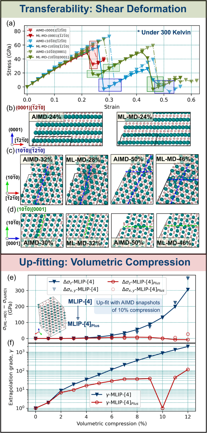
a Comparison of AIMD (dash-dotted line) and ML-MD (solid line) stress/strain curves for TiB2 subject to (0001)\([\overline{1}2\overline{1}0],(10\overline{1}0)[\overline{1}2\overline{1}0]\), and \((10\overline{1}0)[0001]\) room-temperature atomic-scale shear deformation. b–d Representative snapshots at strain steps marked by shaded rectangles in a. The dashed lines in b–d guide the eye for slip directions described in the text. e Differences in ML-MD and AIMD stresses (σ(ML-MD) − σ(AIMD)), resolved in the basal plane and [0001] direction (σx,y and σz) of TiB2 subject to room-temperature volumetric compression, plotted as a function of the compression percentage. f Blue and red data points indicate maximum extrapolation grades returned by MLIP-[4] and its up-fitted version, MLIP-[4]Plus, during TiB2 compression.
The shear strengths predicted by ML-MD for (0001)\([\overline{1}2\overline{1}0],(10\overline{1}0)[\overline{1}2\overline{1}0]\), and \((10\overline{1}0)[0001]\) deformation, (49, 57, and 51 GPa), are ≈ 8% lower than AIMD values (58, 72, and 68 GPa). Nevertheless, shear-induced structural changes observed during ML-MD correctly reproduce AIMD results (Fig. 8b–d).
When subject to (0001)[\(\overline{1}2\overline{1}0\)] shearing, TiB2 undergoes slip on the basal plane. The mechanism—activated for (0001)[\(\overline{1}2\overline{1}0\)] shear strain of ≈ 24% – restores atoms to their ideal lattice sites (Fig. 8b). \((10\overline{1}0)[\overline{1}2\overline{1}0]\) shearing induces plastic flow on both \((\overline{1}2\overline{1}0)[10\overline{1}0]\) and \((10\overline{1}0)[\overline{1}2\overline{1}0]\) slip systems. The mechanisms are activated at strains near 30% and 50% (Fig. 8c). Both are accompanied by displacements of Ti and B atoms from ideal TiB2 lattice sites. Similar to the results in (Fig. 8c), shearing along \((10\overline{1}0)[0001]\) activates different slip systems (Fig. 8d). TiB2(0001) lattice layers glide along \([10\overline{1}0]\) at ≈ 30% strain. A further increase in strain to ≈ 50% induces glide of \((10\overline{1}0)\) planes along the [0001] direction. The latter process results in significant displacements of B atoms and formation of stacking faults, as indicated by horizontal green lines in Fig. 8d (panels on the right).
The excellent agreement between ML-MD and AIMD stress/strain curves within the elastic shear response, accompanied by reasonably good agreement near TiB2 yielding, suggests that up-fitting our MLIP[4] to accurately model shear deformation would benefit from adding configurations near TiB2’s shear instabilities to the training set.
-
Room-temperature volumetric compression ofTiB2. Training on snapshots of compressed structures may be important not only for simulations of e.g., uniaxial compression or nanoindentation, but also in order to correctly account for Poisson’s contraction during tensile deformation. For TiB2, the relatively low Poisson’s ratio (Table 2) is manifested by a rather small lateral shrinkage of the supercell during nanoscale tensile testing simulations. Here we simulate severe volumetric compression of TiB2 at room temperature. All lattice vectors are compressed by up to 12% to show rapidly growing γ values and suggest how to improve MLIP reliability by up-fitting.
As shown in Fig. 8e, f, compression-induced stresses along main crystallographic directions are indeed extremely large. In AIMD, they exceed 50 GPa for a 5% compression and reach ≈ 150 GPa for a 10% compression. Our MLIP yields satisfactory agreement with AIMD for volumetric compression of 1–2%, with stress tensor components differing from ab initio values by less than 1.83 GPa (9.57%) and γ indicating reliable extrapolation (γ≤10 = γreliable). A further increase in compression to 10%, however, causes increasing deviations from AIMD stresses and γ ≈ 102–103.
We illustrate the effect of up-fitting by producing a new MLIP (MLIP-[4]Plus) which learns from AIMD snapshots of 10% volumetrically-compressed TiB2 (added to the LS of MLIP-[4]). This not only greatly improves accuracy for the 10% compression (stress differences are maximum 0.79 GPa (0.48%) and γ ≤ 2) but also within the entire tested compression range (see red data points in Fig. 8e, f).
-
Surface energies of TiB2.
Although our training set did not contain ideal surfaces, environments describing TiB2’s fracture may facilitate reasonable predictions for energies of low-index surfaces. To test this hypothesis, we evaluate the energies of formation, Esurf, of (0001), \((\overline{1}2\overline{1}0)\), and (10\(\overline{1}0\)) surfaces, i.e., orthogonal to simulated tensile loading directions (Section MLIPs’validation against atomic scale tensile tests–Size effects in tensile response of TiB2).
The MLIP-predicted Esurf are consistent with equivalently produced ab initio values (Table 4). The differences are relatively small: 0.03 J m−2 (1.40%) for Esurf(0001), 0.04 J m−2 (1.68%) for \({E}_{{{{\rm{surf}}}}}(\overline{1}2\overline{1}0)\)), and 0.13 J m−2 (5.75%) for \({E}_{{{{\rm{surf}}}}}(10\overline{1}0)\), as underlined also by low extrapolation grades (γ < γreliable). ML-MS and DFT calculations of the present work indicate that the TiB\({}_{2}(\overline{1}2\overline{1}0)\) surface is energetically more stable than the basal plane. This is surprising, given that formation of (\(\overline{1}2\overline{1}0\)) surfaces requires breaking strong, covalent B-B bonds. That the basal plane of TiB2 is not the one with lowest energy has also been indicated by previous DFT tudies73,74. Nevertheless, MLIP up-fitting on higher-accuracy DFT data would be needed to verify the relationship among TiB2 surface energies.
Table 4 Transferability of the here-developed MLIP (MLIP-[4]) in molecular statics (MS) calculations of surface energies, Esurf (J m−2), for low-index surfaces of TiB2 -
Off-stoichiometricTiB2structures and other phases. Our MLIP was trained to snapshots of TiB2 (AlB2-type phase, P6/mmm) with a perfect stoichiometry (speaking of the entire supercell). Visualization of the training set (Fig. 3c), however, indicates the presence of atomic environments with various Ti-to-B ratios as well as bond lengths and angles different from those in TiB2. This may be useful for simulations of e.g., vacancy-containing TiB2 structures commonly reported by synthesis36 or other phases in the Ti–B phase diagram75.
To investigate transferability to other phases, we use MS calculations to find the ground-state of known phases from the Ti–B phase diagram75,76: Ti2B (tetragonal, I4/mcm), Ti3B4 (orthorhombic, Immm), and TiB (orthorhombic Pnma) (The supercell sizes are always ≈ 700 atoms, i.e., comparable to that used for TiB2.). Additionally, we equilibrate the TiB2 phase with Ti, B, or combined Ti and B vacancies: Ti36B71, Ti35B72, and Ti35B70. For all calculations, extrapolation grades (γ ≈ 102–104) are far beyond reliable extrapolation. In terms of total energies (Etot), and lattice parameters (a, b, c), the largest deviation from ab initio values is exhibited by Ti3B4 (10% and 2.5% differences on Etot and c, respectively).
Simulations of other stoichiometries and phases therefore require up-fitting (not necessarily due to poor accuracy but especially due to high uncertainty, γ ≫ γreliable). To illustrate the up-fitting effect, MLIP-[4] learns from additional ab initio snapshots: from 0 K equilibration of a 780-atom Ti3B4 supercell. Prior to up-fitting, equilibration of Ti3B4 yields γ≥104. Afterwards, γ ≤ 5 < γreliable and Etot, a and c deviate from ab initio values by 4.18%, 0.07%, and 0.73%.

Viability of our training strategy for modelling tensile deformation in other ceramics
To illustrate general applicability of the proposed training strategy, we develop MLIPs for 5 other ceramic systems. Once more, we emphasize that the developed MLIPs are primarily targeted to simulations of uniaxial tensile loading at room temperature. The chosen materials are
-
hexagonal α-TaB272, which serves as an example of changing the transition metal while keeping the same crystal structure,
-
hexagonal ω-WB272 and γ-ReB272, i.e., examples of changing the transition metal as well as the phase,
-
cubic NaCl-type TiN67, which serves as example of ceramic system with different non-metal species, different lattice symmetry, and bonding character that is less covalent but more ionic and metallic than TiB2 and diborides in general,
-
orthorhombic, nanolaminated Ti2AlB2 (a MAB phase77), which is example of ternary system with different crystal structure and mixture of ceramic-like and metallic-like bonding.
Training data generation, up-fitting, and validation follow steps carried out for TiB2 in Sections Training procedure and fitting initial MLIPs–MLIPs’ up-fitting for nanoscale tensile tests. Again, the validation consists in (i) evaluating fitting and validation errors with respect to the training set and a meaningful validation set, (ii) comparing the predicted physical properties with equivalently calculated ab initio values, and (iii) monitoring the extrapolation grade during ML-MD simulations.
Fitting and validation errors of energies, forces, and stresses (RMSE < 3 meV atom −1, < 0.15 eV Å−1, and < 0.25 GPa, respectively) are similar to those evaluated for TiB2 in Section Training procedure and fitting initial MLIPs and close to the accuracy of the AIMD training set. Extrapolation grades for all configurations in the validation set are below the accurate extrapolation threshold (γ < 2).
Figure 9 exemplifies validation of ML-MD tensile-stress/elongation curves against corresponding atomic-scale AIMD results. The intention is to demonstrate applicability of our training approach to different ceramic systems. Hence, we omit discussion of deformation and fracture mechanisms which, however, are consistent with AIMD results. The time-averaged stresses recorded during ML-MD tensile tests differ from the corresponding AIMD values by 0–3.3 GPa, yielding statistical errors RMSE ≈ 2.0 GPa, R2 ≈ 0.99. The discrepancy is partly due to stochastic stress fluctuations, which may also onset fracture at slightly different strains in independent MD runs (compare ML-MD and AIMD results for TaB2, ReB2, and TiN in Fig. 9). Previous molecular dynamics tensile-testing investigations demonstrated that the statistical uncertainties on TiN elongation at fracture are comparable to the strain increment68.

a α-TaB2, b ω-WB2, c γ-ReB2, d NaCl-type TiN, and e the orthorhombic Ti2AlB2 MAB phase, as illustrated by stress/strain curves for room-temperature uniaxial tensile deformation. Specifically, the [0001] and the [001] loading directions are chosen as representative examples for hexagonal systems (TaB2, WB2, ReB2) and for the cubic and the orthorhombic systems (TiN, Ti2AlB2), respectively. The supercell sizes and computational setup are equivalent to the atomic scale tensile tests for TiB2, defined by the first bullet point in Section MLIPs’ up-fitting for nanoscale tensile tests. Note that the stress values should not be over-interpreted, as they were obtained for atomic scale supercells (to make a fair comparison with ab initio data) and---in case of negligible size effects---are the ideal upper bounds attainable by a perfect single crystal.
The theoretical tensile strengths of TaB2, WB2, ReB2, TiN, and Ti2AlB2 predicted by ML-MD are 40.3, 50.8, 76.2, 36.7, and 16.5 GPa, respectively. These values differ from those obtained via AIMD by maximum 8%. The corresponding ML-MD and AIMD tensile toughness values deviate by maximum 5%. Extrapolation grades during all ML-MD simulations indicate reliable extrapolation (γ ≤ 5 < γreliable ≈ 10) and remain of similar magnitude also during ML-MD tensile tests on supercells with S1-size (see second bullet point in Section MLIPs’ up-fitting for nanoscale tensile tests).
The results in Fig. 9 suggest general applicability of our approach for development of MLIPs able to describe tensile deformation and fracture in hard ceramics. Specifically, our MLIPs correctly reproduce AIMD results of stress/strain curves and fracture mechanisms in different ceramic systems subject to tensile deformation. Extrapolation grades during all ML-MD tensile tests (both atomic and nanoscale) are of similar magnitude as for TiB2, hence indicating reliable extrapolation and realistic deformation and fracture processes.
Summary and outlook
We proposed a strategy for the development of MLIPs specifically trained to description of deformation and fracture in tensile-loaded ceramic monocrystals. TiB2 served as a model ceramic system. Training data generation, fitting, and validation procedure were performed within the moment tensor potential (MTP) formalism. MLIP-based molecular dynamics tensile-testing investigations have been carried out from the atomic scale ( ≈ 103 atoms) to the nanoscale ( ≈ 104–106 atoms). Furthermore, we discussed the MLIP’s transferability to, e.g., description of TiB2 subject to different loading conditions or different Ti-B phases, as well as the viability of the here-proposed training strategy for developing MLIPs of other ceramics.
Key findings are summarized below.
MLIP development:
-
1.
MLIPs for simulations of tensile deformation until fracture can be trained following the scheme in Fig. 1, based on snapshots from finite-temperature AIMD simulations of sequentially elongated single-crystal models with sizes of ≈ 103 atoms. An analogous training approach may be applicable to other loading conditions (e.g., shearing) and ceramics in different stoichiometries and crystalline phases (e.g., diborides, nitrides, MAB phases).
-
2.
The applicability of MLIPs to description of tensile deformation and Poisson’s contraction at the nanoscale requires up-fitting. This is due to, e.g., nucleation of extended defects being hindered by the small size of AIMD supercells used for generation of training sets. We propose to generate additional ab initio data by room-temperature and elevated-temperature (1200 K) AIMD: imposing a large strain along one lattice vector, initializing atoms at ideal lattice sites, and equilibrating the supercell under fixed volume and shape.
-
3.
MLIPs fitted to room-temperature tensile dataset may be transferable to simulate other loading conditions; here we show examples of high-temperature tensile deformation and room-temperature shear deformation at the atomic scale. Contrarily, up-fitting is certainly required for simulations of volumetric compression, other phases and stoichiometries.
Predictions forTiB2:
-
1.
Our calculations indicate elastic isotropy of TiB2’s basal plane at 300 and 1200 K.
-
2.
The directional dependence of mechanical properties in (initially) dislocation-free supercells qualitatively changes from the atomic to the nanoscale. However, all predicted properties rapidly saturate for supercell sizes increasing from ≈ 104 to ≈ 106 atoms. At 300 K, theoretical tensile strengths during [0001], \([10\overline{1}0]\), and \([\overline{1}2\overline{1}0]\) deformation reach 51–56 GPa.
-
3.
Nanoscale MD simulations provide insights into crack nucleation and growth mechanisms. Subject to [0001] tensile loading, Ti/B2 layer delamination induces opening of nm-sized voids which rapidly coalesce, inducing formation of few-nm-size cracks inside the material. Fracture surfaces align predominantly with basal planes, {0001}, and first order pyramidal planes, {10\(\overline{1}\)1}.
-
4.
Considering deformation within the basal plane, \([10\overline{1}0]\) tensile test (i.e., loading in the direction of strong B–B bonds), most often induces crack deflection, formation of V-shaped defects, and fracture at \(\{11\overline{2}2\}\) family of surfaces. Contrarily, the \([\overline{1}2\overline{1}0]\) tensile deformation induces fracture at {10\(\overline{1}\)0} prismatic planes.
The example of TiB2 together with additional ML-MD tensile tests done on other ceramics (TaB2, WB2, ReB2, TiN, Ti2AlB2) indicate the viability of the here-proposed MLIP training strategy. Our approach may be extendable also to other MLIP formalisms. The predictions of nanoscale deformation and fracture in TiB2 presented in this work may aid interpretation of future mechanical-testing experiments. Several previous studies have already demonstrated the importance of MD simulations for elucidating microscopy observations refs. 78,79,80. Follow-up work could focus on MLIP up-fitting for modelling more complex problems as, e.g., Mode-I loading of native flaws and nanosized cracks.
Methods
Ab initio calculations
Zero Kelvin ab initio calculations as well as finite-temperature Born-Oppenheimer ab initio molecular dynamics (AIMD) were carried out using VASP81 together with the projector augmented wave (PAW)82 method and the Perdew-Burke-Ernzerhof exchange-correlation functional revised for solids (PBEsol)83. All AIMD calculations employed plane-wave cut-off energies of 300 eV and Γ-point sampling of the reciprocal space.
Supercells. The model of TiB2 was based on the AlB2-type structure (P6/mmm). The 720-atom (240 Ti + 480 B) supercell—used to generate the training/learning/validation dataset—had size of ≈ (1.5 × 1.6 × 2.6) nm3, with x, y, z axes chosen to satisfy the following crystallographic relationships: \(x\parallel [10\overline{1}0],y\parallel [\overline{1}2\overline{1}0],z\parallel [0001]\). Similar supercells—with 720 atoms (240 M + 480 B)—were used in Section Viability of our training strategy for modelling tensile deformation in other ceramics for TaB2, WB2, and ReB2, where the latter two are in the ω and γ phase72, respectively. Cubic (fcc, Fm\(\overline{3}{{{\rm{m}}}}\)) TiN67 was modelled in a 360-atom (180 Ti + 180 N) supercell, with x, y, and z axes aligned with the [100], [010], and [001] directions. The orthorhombic (Cmcm) Ti2AlB277 was modelled in a 720-atom supercell (288 Ti + 144 Al + 288 B), oriented in the same way as the TiN supercell.
Equilibration of TiB2 at 300 and 1200 K was performed in 2 steps: (i) 10 ps AIMD isobaric-isothermal (NPT) simulation with Parrinello-Rahman barostat84 and Langevin thermostat, and (ii) a 2 ps for 300 K, 4 ps for 1200 K AIMD run within the canonical (NVT) ensemble based on Nosé-Hoover thermostat, using time-averaged lattice parameters from the NPT simulation (see the Supplementary Fig. 1). TaB2, WB2, ReB2, TiN, and Ti2AlB2 were equilibrated at 300 K using the same approach.
Computational setup for simulations of TiB2’s [0001], \([10\overline{1}0]\), and \([\overline{1}2\overline{1}0]\) tensile deformation and (0001)\([\overline{1}2\overline{1}0],(10\overline{1}0)[\overline{1}2\overline{1}0]\), and \((10\overline{1}0)[0001]\) shear deformation (all with Γ point sampling) followed refs. 61,67,85. Specifically, the equilibrated supercell was elongated or sheared in the desired direction using strain increments of 2%. Poisson’s contraction effects were not considered in AIMD simulations. The supercells are equilibrated for 3 ps at each deformation step. Stress tensor components were calculated as averages of the final 0.5 ps. The same approach was used to simulate tensile deformation in TaB2, WB2, ReB2, TiN, and Ti2AlB2.
Room-temperature elastic constants, Cij, of TiB2 were evaluated following ref. 86, based on a second-order polynomial fit of the [0001], [10\(\overline{1}0\)], and [\(\overline{1}2\overline{1}0\)] stress/strain data (C11, C12, C13, C33) and of the (0001)\([\overline{1}2\overline{1}0],(10\overline{1}0)[\overline{1}2\overline{1}0]\), and \((10\overline{1}0)[0001]\) shear stress/strain data (C44), considering strains between 0 and 4%.
Simulations of TiB2’s room-temperature volumetric compression were carried out for a 720-atom TiB2 supercell maintained at 300 K (for 2 ps) within the NVT ensemble. The surface energies were calculated at zero Kelvin using a 60-atom TiB2 supercell (with a 3 × 3 × 1 k-mesh and cut-off energy of 300 eV) together with a 10 Å vacuum layer. The supercells were fully relaxed until forces on atoms were below 10−2 eV Å−1 and the total energy was converged with accuracy of 10−5 eV per supercell. Other ground-state and higher-energy structures from the Ti–B phase diagram (Ti2B, Ti3B4, TiB, TiB12, etc.) were fully relaxed at 0 K starting from lattice parameters and atomic positions from the Materials Project76.
Development of machine-learning interatomic potentials (MLIPs)
We used the moment tensor potential (MTP) formalism, as implemented in the mlip-2 package87. Training data generation and general workflow are detailed in the Section Training procedure and fitting initial MLIPs and Fig. 1. Training/learning/validation sets included only equilibrated configurations: the initial part (5%) of NVT rus was discarded.
MLIPs were fitted based on the 16g MTPs (referring to the highest degree of polynomial-like basis functions in the analytic description of the MTP23), using the Broyden-Fletcher-Goldfarb-Shanno method88 with 1500 iterations and 1.0, 0.01 and 0.01 weights for total energy, stresses and forces in the loss functional. A cutoff radius of 5.5 Å was employed, similar to other recent MLIP studies19,89. Tests using larger cutoffs, 7.4 and 10.0 Å did not show notable changes in accuracy. Expansion of a training set by selection of configurations from a learning set (LS), was done using the select add command of the mlip-2 package. Specifically, all configurations in the LS were ordered by their extrapolation grade (γ28) and maximum 15 from the upper 20% was selected to expand the training set.
Details of MLIPs developed in this work (summarized in Fig. 1c) are given below.
-
MLIP-[0001], (MLIP-\([10\overline{1}0]\), and MLIP-\([\overline{1}2\overline{1}0]\)): trained on AIMD snapshots of TiB2 subject to room-temperature tensile loading in the [0001] (\([10\overline{1}0],[\overline{1}2\overline{1}0]\)) direction. See Section Training procedure and fitting initial MLIPs and MLIPs’validation against atomic scale tensile tests.
-
MLIP-[1]: up-fitting MLIP-[0001], learning from the final TSs of MLIP-[10\(\overline{1}0\)] and MLIP-[\(\overline{1}2\overline{1}0\)]. See Section MLIPs’ up-fitting for nanoscale tensile tests.
-
MLIP-[2] and MLIP-[3]: up-fitting MLIP-[1], learning from AIMD snapshots of TiB2 equilibrated at 1200 K (MLIP-[2]), and sequentially elongated in the [0001] direction until cleavage (MLIP-[3]). See Section MLIPs’ up-fitting for nanoscale tensile tests.
-
MLIP-[4]: up-fitting MLIP-[1], learning from AIMD snapshots of TiB2 elongated by 150% in the [0001] direction, initializing atoms at ideal lattice sites and equilibrating at 300 and 1200 K under fixed volume and shape. See Section MLIPs’ up-fitting for nanoscale tensile tests–Otherloading conditions and MLIP’s transferability.
Molecular dynamics with MLIPs (ML-MD)
ML-MD calculations were performed with the LAMMPS code90 interfaced with mlip-2 package87, which allows using MTP-type MLIPs (specified in the pair_style command). Additionally, the active learning state file (state.als, for details see the mlip-2 documentation (https://gitlab.com/ashapeev/mlip-2-paper-supp-info)) was used to output the extrapolation grade, γ, values during the simulations.
Computational setup of atomic scale ML-MD tensile and shear tests (at 300 or 1200 K) was equivalent to AIMD. Stress tensor components and elastic constants were calculated in the same way as described above in case of AIMD.
Nanoscale ML-MD tensile tests at 300 or 1200 K used supercells with 12,960 atoms (S1); 141,120 atoms (S2); 230,400 atoms (S3); and 432,000 atoms (S4); with dimensions of about (1.5 × 1.6 × 2.6) nm3, (4.6 × 4.7 × 5.1) nm3, (10.6 × 11.0 × 10.3) nm3, (12.1 × 12.6 × 12.9) nm3, and (15.2 × 15.8 × 15.4) nm3, respectively. Prior to simulating mechanical deformation, the supercells were equilibrated for 5 ps at the target temperature using the isobaric-isothermal (NPT) ensemble coupled to the Nosé-Hoover thermostat with a 1 fs time step. Tensile loading was simulated by deforming the supercell with a constant strain rate (50 Å s−1), accounting for lateral contraction (Poisson’s effect) in the NPT ensemble.
Atomic scale volumetric compression simulations used supercell sizes and deformation approach equivalent to what was described above for AIMD. Surface structures and other Ti–B phases were fully relaxed at 0 K using conjugate gradient energy minimization in molecular statics (MS).
Visualization and structural analysis
The OVITO package91 allowed us to visualize and analyze selected AIMD and ML-MD trajectories. In particular, we looked at (i) Radial pair distribution functions (with a cut-off radius of 5.5 Å), (ii) Elastic strain maps and (iii) Atomic strain maps (with cut-off radius of ± 0.1 Å). For details see the OVITO documentation.
Data availability
The related files are compressed as “ Available_Data.zip ” and submitted as part of Supplementary Materials, the details description can be found at the end of “ Supplementary_Materials.pdf ”, as well as “ READ_ME.txt ” in the compressed folder. The more specific explanation and help will be made available upon request.
Change history
18 April 2024
A Correction to this paper has been published: https://doi.org/10.1038/s41524-024-01276-9
References
Bianchini, F., Glielmo, A., Kermode, J. & De Vita, A. Enabling QM-accurate simulation of dislocation motion in γ-Ni and α-Fe using a hybrid multiscale approach. Phys. Rev. Mater. 3, 043605 (2019).
Zhao, Y. Understanding and design of metallic alloys guided by phase-field simulations. Npj Comput. Mater. 9, 94 (2023).
Sivaraman, G. et al. Machine-learned interatomic potentials by active learning: amorphous and liquid hafnium dioxide. Npj Comput. Mater. 6, 104 (2020).
Fiedler, L. et al. Predicting electronic structures at any length scale with machine learning. Npj Comput. Mater. 9, 115 (2023).
Rassoulinejad-Mousavi, S. M. & Zhang, Y. Interatomic potentials transferability for molecular simulations: a comparative study for platinum, gold and silver. Sci. Rep. 8, 2424 (2018).
Bianchini, F., Kermode, J. & De Vita, A. Modelling defects in Ni–Al with EAM and DFT calculations. Model. Simul. Mat. Sci. Eng. 24, 045012 (2016).
Proville, L., Rodney, D. & Marinica, M.-C. Quantum effect on thermally activated glide of dislocations. Nat. Mater. 11, 845–849 (2012).
Deringer, V. L., Caro, M. A. & Csányi, G. Machine learning interatomic potentials as emerging tools for materials science. Adv. Mater. 31, 1902765 (2019).
Zuo, Y. et al. Performance and cost assessment of machine learning interatomic potentials. J. Phys. Chem. A 124, 731–745 (2020).
Drautz, R. Atomic cluster expansion for accurate and transferable interatomic potentials. Phys. Rev. B 99, 014104 (2019).
Smith, J. S., Isayev, O. & Roitberg, A. E. ANI-1: an extensible neural network potential with DFT accuracy at force field computational cost. Chem. Sci. 8, 3192–3203 (2017).
Shapeev, A. V., Podryabinkin, E. V., Gubaev, K., Tasnádi, F. & Abrikosov, I. A. Elinvar effect in β-Ti simulated by on-the-fly trained moment tensor potential. N. J. Phys. 22, 113005 (2020).
Nishiyama, T., Seko, A. & Tanaka, I. Application of machine learning potentials to predict grain boundary properties in fcc elemental metals. Phys. Rev. Mater. 4, 123607 (2020).
Deng, F., Wu, H., He, R., Yang, P. & Zhong, Z. Large-scale atomistic simulation of dislocation core structure in face-centered cubic metal with Deep Potential method. Comput. Mater. Sci. 218, 111941 (2023).
Mori, H. & Ozaki, T. Neural network atomic potential to investigate the dislocation dynamics in bcc iron. Phys. Rev. Mater. 4, 040601 (2020).
Rosenbrock, C. W. et al. Machine-learned interatomic potentials for alloys and alloy phase diagrams. Npj Comput. Mater. 7, 24 (2021).
Zong, H., Pilania, G., Ding, X., Ackland, G. J. & Lookman, T. Developing an interatomic potential for martensitic phase transformations in zirconium by machine learning. Npj Comput. Mater. 4, 48 (2018).
Li, X.-G. et al. Quantum-accurate spectral neighbor analysis potential models for Ni-Mo binary alloys and fcc metals. Phys. Rev. B 98, 094104 (2018).
Tasnádi, F., Bock, F., Tidholm, J., Shapeev, A. V. & Abrikosov, I. A. Efficient prediction of elastic properties of Ti0.5Al0. 5N at elevated temperature using machine learning interatomic potential. Thin Solid Films 737, 138927 (2021).
Thompson, A. P., Swiler, L. P., Trott, C. R., Foiles, S. M. & Tucker, G. J. Spectral neighbor analysis method for automated generation of quantum-accurate interatomic potentials. J. Comput. Phys. 285, 316–330 (2015).
Behler, J. Constructing high-dimensional neural network potentials: a tutorial review. Int. J. Quantum Chem. 115, 1032–1050 (2015).
Bartók, A. P., Payne, M. C., Kondor, R. & Csányi, G. Gaussian approximation potentials: The accuracy of quantum mechanics, without the electrons. Phys. Rev. Lett. 104, 136403 (2010).
Shapeev, A. V. Moment tensor potentials: A class of systematically improvable interatomic potentials. Multiscale Model. Simul. 14, 1153–1173 (2016).
Seko, A., Togo, A. & Tanaka, I. Group-theoretical high-order rotational invariants for structural representations: Application to linearized machine learning interatomic potential. Phys. Rev. B 99, 214108 (2019).
Qamar, M., Mrovec, M., Lysogorskiy, Y., Bochkarev, A. & Drautz, R. Atomic cluster expansion for quantum-accurate large-scale simulations of carbon. J. Chem. Theory Comput. 19, 5151–5167 (2023).
Rowe, P., Csányi, G., Alfe, D. & Michaelides, A. Development of a machine learning potential for graphene. Phys. Rev. B 97, 054303 (2018).
Cohn, D. A., Ghahramani, Z. & Jordan, M. I. Active learning with statistical models. J. Artif. Intell. 4, 129–145 (1996).
Podryabinkin, E. V. & Shapeev, A. V. Active learning of linearly parametrized interatomic potentials. Comput. Mater. Sci. 140, 171–180 (2017).
Gubaev, K., Podryabinkin, E. V. & Shapeev, A. V. Machine learning of molecular properties: Locality and active learning. Tj. Chem. Phys. 148, 241727 (2018).
Lysogorskiy, Y., Bochkarev, A., Mrovec, M. & Drautz, R. Active learning strategies for atomic cluster expansion models. Phys. Rev. Mater. 7, 043801 (2023).
Lysogorskiy, Y. et al. Performant implementation of the atomic cluster expansion (PACE) and application to copper and silicon. npj Comput. Mater. 7, 1–12 (2021).
Luo, G. A review of automatic selection methods for machine learning algorithms and hyper-parameter values. Netw. Model. Anal. Health Inform. Bioinform. 5, 1–16 (2016).
Salem, M., Cowan, M. J. & Mpourmpakis, G. Predicting segregation energy in single atom alloys using physics and machine learning. ACS omega 7, 4471–4481 (2022).
Fang, J. et al. Machine learning accelerates the materials discovery. Mater. Today Commun. 104900 (2022).
Ribeiro, F. & Gradvohl, A. L. S. Machine learning techniques applied to solar flares forecasting. Astron. Comput. 35, 100468 (2021).
Magnuson, M., Hultman, L. & Högberg, H. Review of transition-metal diboride thin films. Vacuum 196, 110567 (2022).
Holleck, H. Material selection for hard coatings. J. Vac. Sci. Technol. 4, 2661–2669 (1986).
Golla, B. R., Mukhopadhyay, A., Basu, B. & Thimmappa, S. K. Review on ultra-high temperature boride ceramics. Prog. Mater. Sci. 111, 100651 (2020).
Wang, C., Akbar, S., Chen, W. & Patton, V. Electrical properties of high-temperature oxides, borides, carbides, and nitrides. J. Mater. Sci. 30, 1627–1641 (1995).
Sevik, C., Bekaert, J., Petrov, M. & Milošević, M. V. High-temperature multigap superconductivity in two-dimensional metal borides. Phys. Rev. Mater. 6, 024803 (2022).
Wiedemann, R., Oettel, H. & Jerenz, M. Structure of deposited and annealed TiB2 layers. Surf. Coat. Technol. 97, 313–321 (1997).
Hofmann, W. & Jäniche, W. Die struktur von aluminiumborid AlB2. Z. f.ür. Physikalische Chem. 31, 214–222 (1936).
Eorgan, J. & Fern, N. Zirconium diboride coatings on tantalum. JOM 19, 6–11 (1967).
Norton, J. T., Blumenthal, H. & Sindeband, S. Structure of diborides of titanium, zirconium, columbium, tantalum and vanadium. JOM 1, 749–751 (1949).
Mikula, M. et al. Mechanical properties of superhard TiB2 coatings prepared by DC magnetron sputtering. Vacuum 82, 278–281 (2007).
Geng, J. et al. Microstructural and mechanical anisotropy of extruded in-situ TiB2/2024 composite plate. Mater. Sci. Eng. 687, 131–140 (2017).
Zhang, T. F., Gan, B., Park, S.-m, Wang, Q. M. & Kim, K. H. Influence of negative bias voltage and deposition temperature on microstructure and properties of superhard TiB2 coatings deposited by high power impulse magnetron sputtering. Surf. Coat. Technol. 253, 115–122 (2014).
Fuger, C. et al. Revisiting the origins of super-hardness in TiB2+z thin films–impact of growth conditions and anisotropy. Surf. Coat. Technol. 446, 128806 (2022).
Munro, R. G. Material properties of titanium diboride. J. Res. Natl Inst. Stan. 105, 709 (2000).
Chen, Z. et al. Room-temperature deformation of single crystals of ZrB2 and TiB2 with the hexagonal AlB2 structure investigated by micropillar compression. Sci. Rep. 11, 14265 (2021).
Zhang, T. et al. Preparation of highly-dense TiB2 ceramic with excellent mechanical properties by spark plasma sintering using hexagonal TiB2 plates. Mater. Res. Express 6, 125055 (2019).
Zhou, Y., Wang, J., Li, Z., Zhan, X. & Wang, J. First-principles investigation on the chemical bonding and intrinsic elastic properties of transition metal diborides TMB2 (TM = Zr, Hf, Nb, Ta, and Y). Ultra-High Temperature Ceramics: Materials for Extreme Environment Applications 60–82 (2014).
Dai, F.-Z. & Zhou, Y. Effects of transition metal (TM = Zr, Hf, Nb, Ta, Mo, W) elements on the shear properties of TMB2s: A first-principles investigation. Comput. Mater. Sci. 117, 266–269 (2016).
Zhang, X., Luo, X., Li, J., Hu, P. & Han, J. The ideal strength of transition metal diborides TMB2 (TM = Ti, Zr, Hf): plastic anisotropy and the role of prismatic slip. Scr. Mater. 62, 625–628 (2010).
Attarian, S. & Xiao, S. Development of a 2NN - MEAM potential for TiB system and studies of the temperature dependence of the nanohardness of TiB2. Comput. Mater. Sci. 201, 110875 (2022).
Attarian, S.Multiscale modeling of Ti/TiB composites. Ph.D. thesis, The University of Iowa (2021).
Timalsina, B.Development of Eam and Rf-MEAM Interatomic Potential for Zirconium Diboride. Ph.D. thesis, Missouri State University (2021).
Daw, M. S., Lawson, J. W. & Bauschlicher Jr, C. W. Interatomic potentials for zirconium diboride and hafnium diboride. Comput. Mater. Sci. 50, 2828–2835 (2011).
Chicco, D., Warrens, M. J. & Jurman, G. The coefficient of determination R-squared is more informative than SMAPE, MAE, MAPE, MSE and RMSE in regression analysis evaluation. PeerJ Comput. Sci. 7, e623 (2021).
Podryabinkin, E., Garifullin, K., Shapeev, A. & Novikov, I. MLIP-3: Active learning on atomic environments with moment tensor potentials. J. Chem. Phys. 159, 084112 (2023).
Koutná, N. et al. Atomistic mechanisms underlying plasticity and crack growth in ceramics: a case study of \({{{\rm{AlN}}}}\)/TiN superlattices. Acta Mater. 229, 117809 (2022).
Nakano, K., Imura, T. & Takeuchi, S. Hardness anisotropy of single crystals of IVa-diborides. Jpn. J. Appl. Phys. 12, 186 (1973).
Hodapp, M. & Shapeev, A. In operando active learning of interatomic interaction during large-scale simulations. Mach. Learn. Sci. technol. 1, 045005 (2020).
Freitas, R. & Cao, Y. Machine-learning potentials for crystal defects. MRS Commun. 12, 510–520 (2022).
Paul, B. et al. Plastic deformation of single crystals of CrB2, TiB2 and ZrB2 with the hexagonal AlB2 structure. Acta Mater. 211, 116857 (2021).
Waldl, H. et al. Evolution of the fracture properties of arc evaporated Ti1−xAlxN coatings with increasing Al content. Surf. Coat. Technol. 444, 128690 (2022).
Sangiovanni, D., Tasnádi, F., Johnson, L., Odén, M. & Abrikosov, I. Strength, transformation toughening, and fracture dynamics of rocksalt-structure Ti1−x Alx N (0 x 0.75) alloys. Phys. Rev. Mater. 4, 033605 (2020).
Sangiovanni, D. G. et al. Descriptor for slip-induced crack blunting in refractory ceramics. Phys. Rev. Mater. 7, 103601 (2023).
Jiao, Y., Huang, L. & Geng, L. Progress on discontinuously reinforced titanium matrix composites. J. Alloy. Compd. 767, 1196–1215 (2018).
Dub, S. et al. Mechanical properties of single crystals of transition metals diborides TMB2 (TM= Sc, Hf, Zr, Ti). experiment and theory. J. Superhard Mater. 39, 308–318 (2017).
Lei, J. et al. Synthesis and high-pressure mechanical properties of superhard rhenium/tungsten diboride nanocrystals. ACS nano 13, 10036–10048 (2019).
Leiner, T. et al. On energetics of allotrope transformations in transition-metal diborides via plane-by-plane shearing. Vacuum 215, 112329 (2023).
Sun, W., Dai, F., Xiang, H., Liu, J. & Zhou, Y. General trends in surface stability and oxygen adsorption behavior of transition metal diborides (TMB2). J. Mater. Sci. Technol. 35, 584–590 (2019).
Gan, Q. et al. Robust hydrophobic materials by surface modification in transition-metal diborides. ACS Appl. Mater. Interfaces 13, 58162–58169 (2021).
Murray, J., Liao, P. & Spear, K. The B-Ti (boron-titanium) system. Bull. Alloy Phase Diagr. 7, 550–555 (1986).
Jain, A. et al. Commentary: The materials project: A materials genome approach to accelerating materials innovation. APL Mater. 1, 011002 (2013).
Carlsson, A., Rosen, J. & Dahlqvist, M. Theoretical predictions of phase stability for orthorhombic and hexagonal ternary MAB phases. Phys. Chem. Chem. Phys. 24, 11249–11258 (2022).
Koutná, N. et al. Atomistic mechanisms underlying plasticity and crack growth in ceramics: a case study of AlN/TiN superlattices. Acta Mater. 229, 117809 (2022).
Salamania, J. et al. Elucidating dislocation core structures in titanium nitride through high-resolution imaging and atomistic simulations. Mater. Des. 224, 111327 (2022).
Chen, Z. et al. Atomic insights on intermixing of nanoscale nitride multilayer triggered by nanoindentation. Acta Mater. 214, 117004 (2021).
Kresse, G. & Furthmüller, J. Efficient iterative schemes for ab initio total-energy calculations using a plane-wave basis set. Phys. Rev. B 54, 11169 (1996).
Kresse, G. & Joubert, D. From ultrasoft pseudopotentials to the projector augmented-wave method. Phys. Rev. B 59, 1758–1775 (1999).
Perdew, J. P. et al. Restoring the density-gradient expansion for exchange in solids and surfaces. Phys. Rev. Lett. 100, 136406 (2008).
Parrinello, M. & Rahman, A. Polymorphic transitions in single crystals: A new molecular dynamics method. J. Appl. Phys. 52, 7182–7190 (1981).
Sangiovanni, D., Mellor, W., Harrington, T., Kaufmann, K. & Vecchio, K. Enhancing plasticity in high-entropy refractory ceramics via tailoring valence electron concentration. Mater. Des. 209, 109932 (2021).
Sangiovanni, D. G. et al. Temperature-dependent elastic properties of binary and multicomponent high-entropy refractory carbides. Mater. Des. 204, 109634 (2021).
Novikov, I. S., Gubaev, K., Podryabinkin, E. V. & Shapeev, A. V. The MLIP package: moment tensor potentials with MPI and active learning. Mach. learn.: sci. technol. 2, 025002 (2020).
Fletcher, R.Practical methods of optimization (John Wiley & Sons, 2013).
Erhard, L. C., Rohrer, J., Albe, K. & Deringer, V. L. A machine-learned interatomic potential for silica and its relation to empirical models. Npj Comput. Mater. 8, 90 (2022).
Thompson, A. P. et al. LAMMPS - a flexible simulation tool for particle-based materials modeling at the atomic, meso, and continuum scales. Comp. Phys. Comm. 271, 108171 (2022).
Stukowski, A. Visualization and analysis of atomistic simulation data with OVITO–the open visualization tool. Model. Simul. Mat. Sci. Eng. 18, 015012 (2009).
Chen, L. et al. A facile one-step route to nanocrystalline TiB2 powders. Mater. Res. Bull. 39, 609–613 (2004).
Mukaida, M., Goto, T. & Hirai, T. Preferred orientation of TiB2 plates prepared by CVD of the TiCl4+ B2 H6 system. J. Mater. Sci. 26, 6613–6617 (1991).
Kelesoglu, E. & Mitterer, C. Structure and properties of TiB2 based coatings prepared by unbalanced DC magnetron sputtering. Surf. Coat. Technol. 98, 1483–1489 (1998).
Xiang, H., Feng, Z., Li, Z. & Zhou, Y. Temperature-dependence of structural and mechanical properties of TiB2: A first principle investigation. J. Appl. Phys.117 (2015).
Spoor, P. et al. Elastic constants and crystal anisotropy of titanium diboride. Appl. Phys. Lett. 70, 1959–1961 (1997).
Amulele, G. M. & Manghnani, M. H. Compression studies of TiB2 using synchrotron X-ray diffraction and ultrasonic techniques. J. Appl. Phys. 97, 023506 (2005).
Guan, C. & Zhu, H. Theoretical insights into the behaviors of sodium and aluminum on the cathode titanium diboride surfaces. Comput. Mater. Sci. 211, 111535 (2022).
Clayton, J. et al. Deformation and failure mechanics of boron carbide–titanium diboride composites at multiple scales. JOM 71, 2567–2575 (2019).
Fan, H. & El-Awady, J. A. Molecular dynamics simulations of orientation effects during tension, compression, and bending deformations of magnesium nanocrystals. J. Appl. Mech. 82, 101006 (2015).
Acknowledgements
L.C.T. acknowledges the National Academic Infrastructure for Supercomputing in Sweden (NAISS). F.T. acknowledges support from the Knut and Alice Wallenberg Foundation (Wallenberg Scholar grant no. KAW-2018.0194) and from VINNOVA (FunMat-II project grant no. 2022-03071). L.H. acknowledges financial support from the Swedish Government Strategic Research Area in Materials Science on Functional Materials at Linköping University SFO-Mat-LiU No. 2009 00971. Support from Knut and Alice Wallenberg Foundation Scholar Grants KAW2016.0358 and KAW2019.0290 is also acknowledged by L.H. D.G.S. gratefully acknowledges financial support from the Swedish Research Council (VR) through Grant No. VR-2021-04426 and the Competence Center Functional Nanoscale Materials (FunMat-II) (Vinnova Grant No. 2022-03071). N.K. acknowledges the Austrian Science Fund, FWF, (T-1308). The computations handling were enabled by resources provided by the National Academic Infrastructure for Supercomputing in Sweden (NAISS) and the Swedish National Infrastructure for Computing (SNIC) at the National Supercomputer Center (NSC) partially funded by the Swedish Research Council through grant agreements nos. 2022-06725 and 2018-05973, as well as, by the Vienna Scientific Cluster (VSC) in Austria. The authors acknowledge TU Wien Bibliothek for financial support through its Open Access Funding Program. This research was funded in whole or in part by the Austrian Science Fund (FWF) [10.55776/T1308]. For open access purposes, the author has applied a CC BY public copyright license to any author accepted manuscript version arising from this submission.
Author information
Authors and Affiliations
Contributions
S.L. carried out the simulations, analyzed and visualized the data, and wrote the first manuscript draft; L.C.T. and F.T. advised on the methodology, data analysis, and visualization; L.H. and P.H.M. helped to improve the manuscript and to discuss the results with respect to state-of-the art experiments, they also provided financial support; D.G.S. and N.K. designed the project and shaped the manuscript; N.K. provided day-to-day supervision to S.L. All authors commented on the manuscript and helped to revise it.
Corresponding author
Ethics declarations
Competing interests
The authors declare no competing interests.
Additional information
Publisher’s note Springer Nature remains neutral with regard to jurisdictional claims in published maps and institutional affiliations.
Supplementary information
Rights and permissions
Open Access This article is licensed under a Creative Commons Attribution 4.0 International License, which permits use, sharing, adaptation, distribution and reproduction in any medium or format, as long as you give appropriate credit to the original author(s) and the source, provide a link to the Creative Commons licence, and indicate if changes were made. The images or other third party material in this article are included in the article’s Creative Commons licence, unless indicated otherwise in a credit line to the material. If material is not included in the article’s Creative Commons licence and your intended use is not permitted by statutory regulation or exceeds the permitted use, you will need to obtain permission directly from the copyright holder. To view a copy of this licence, visit http://creativecommons.org/licenses/by/4.0/.
About this article

Cite this article
Lin, S., Casillas-Trujillo, L., Tasnádi, F. et al. Machine-learning potentials for nanoscale simulations of tensile deformation and fracture in ceramics. npj Comput Mater 10, 67 (2024). https://doi.org/10.1038/s41524-024-01252-3
Received:
Accepted:
Published:
DOI: https://doi.org/10.1038/s41524-024-01252-3
