
Abstract
Recent efforts on design for four-dimensional (4D) printing have considered the spatial arrangement of smart materials and energy stimuli. The development of multifunctional structures and their desired mechanical/actuation performances require tackling 4D printing from a multi-material design perspective. With the materials distributions there is an opportunity to increase the spectrum of design concepts with computational approaches. The main goal being to achieve the “best” distribution of material properties in a voxelized structure, a computational framework that consists of a finite element analysis-based evolutionary algorithm is presented. It fuses the advantages of optimizing both the materials distribution and material layout within a design space via topology optimization to solve the inverse design problem of finding an optimal design to achieve a target shape change by integrating void voxels. The results demonstrate the efficacy of the proposed method in providing a highly capable tool for the design of 4D-printed active composites.
Introduction
The emergence of increasingly ground-breaking scientific advancement of the additive manufacturing sector over the past decades as well as cutting-edge discoveries in the domain of active materials have birthed a novel class of (meta)material(s): active composites. As its name suggests, active composites consist of at least two different materials, one, if not both1, comprising of a smart material and another passive or inert material. Smart materials are an umbrella term that englobes a variety of materials that can be subjected to transformations in shape as well as other properties such as stiffness, state (of matter), color, etc., with a specific actuation. As present in the literature, these actuations, commonly referred to as energy stimuli, ranges in terms of accessibility and ease of use from heat/temperature2 to humidity, pH, solvent3, electricity4, magnetism5,6, light7, etc. The various classes of smart materials prominently researched include shape memory polymers8, shape memory alloys9, liquid crystal elastomers10,11,12,13 and hydrogels14,15 to name a few.
In the context of active composites, the reaction to an environmental stimulus is largely dependent on the constraints applied to the inert matrix material. In other words, the spatial layout of both materials, also known as the materials distribution, in an active composite is the biggest factor that influences the specific shape changes induced. Conceptually, this provides a massive breakthrough in terms of design in the form of a parameter that opens the door to an almost infinite number of possibilities which were not available when working with unique standard materials. Inversely, this brings with it a complexity in determining the best approach or strategy to attain the optimal materials distribution for a specific need16. This naturally leads to two types of design strategies, knowledge-based design (intuitive) and computational design (possibly counter-intuitive)17. The former takes advantage of experience and knowledge as well as human intuition and understanding of basic problems to provide straightforward solutions for elementary needs that can then be compounded to respond to more complex requirements. Examples include multi-layer designs and basic patterns18. However, the limitation to human intuition as well as the trial-and-error nature of experimentation of this method led to the second category of design, computational design. Conversely, the advances in computer programming and machine-learning capabilities coupled with modeling and simulation approaches can be used to generate a solution that is tailored to achieve a highly complex shape-change while including the notion of ‘optimization’19.
By combining additive manufacturing and active materials under the effect of an energy stimulus, four-dimensional (4D) printing is a booming research domain that require intensive investigations both at the digital and physical levels. The current state-of-the-art technology in 4D printing in terms of manufacturability allows the accurate arrangement of different materials in a single part, especially with material extrusion (i.e., fused filament fabrication20, direct ink writing21,22,23,24,25) and material jetting26 (i.e., PolyJet technique). This leads to potential applications in various industries: soft robotics27, biomedical engineering28, smart actuators29, aerospace technology30, etc. In tackling the design aspect of the application of active composites, one is confronted with a convoluted inverse problem of finding the optimal material or property distribution to obtain a desired shape change which relies heavily on precise numerical models, such as finite element models, and the exploration strategy, in the form of an optimization algorithm. Approaches that were previously considered incorporate various methods founded upon gradient-based topology optimization (TO) including, but not limited to, level-set topology31, graded density optimization32,33, linear elastic TO34, TO with microstructures35, etc. However, the limitations of these methods are apparent when dealing with active materials that are highly non-linear and are subject to large deformations.
Another proponent for a gradient-free method is the design flexibility and simplicity when dealing with discrete variables (discrete materials in this context) as opposed to continuous variables that is practically essential in gradient-based methods. This leads inevitably to design based on voxelized structures where each voxel or polyvoxel (i.e., spatial region formed by joining at least two voxels face to face) corresponds to a specific material36,37,38. Taking the aforementioned fabrication technologies into account, defining clear interfaces between materials during the design process provides a more accurate representation of the corresponding printed parts. But, in the present multi-material modeling, deterministic deformations or the absence of bifurcations are assumed.
As far as non-intuitive design is concerned, a paradigm shift towards data-driven approaches, i.e., attribute-value systems incorporating experimental evaluations dependent on performance metrics with no programmed knowledge of the problem that is being solved, is increasingly apparent. An advantage of this approach is the fact that it is free of human preconceptions and biases when finding a solution39. One such algorithm that is prioritized in combinatorial optimization problems with relatively many variables is the evolutionary algorithm (EA)40,41. It is a nondeterministic method that employs biomimetic techniques revolving around natural selection and evolution to strive towards producing increasingly better ‘individuals’, which correspond to the evaluated solutions, after each generation. Besides fitness-based natural selection, otherwise known as ‘the survival of the fittest’, concepts such as mutation and crossover as well as populations containing ‘parents’ and ‘children’ are appropriated and adapted to each problem.
Recently Hamel et al. (2019)42 used an EA-based design strategy to find the optimal materials distribution for different case studies, all of which yielded good agreement with the inputted target shape change. However, the design variables consisted purely of the materials comprising the active composite: a smart material and an inert material. In this paper, the objective is to expand upon a similar strategy while also including the notion of TO directly in the EA by incorporating void elements as part of the design variables. This fusion of TO with the existing materials distribution optimization strategy allows for a gradient-free method that pushes the limit on the concept of placing the right material at the right place. A computational framework that combines EA with a finite element method (FEM) on a conventional software allows the user to choose from several types of smart materials to launch a case study that yields an optimal solution corresponding to a materials distribution containing three ‘materials’, smart, inert, and void, to obtain a target shape-change. Two cases are tested and illustrated in the following section.
Results and Discussion
Multimaterial active composite
With the proposed computational design framework, we consider and study an active composite in the form of a simple cantilever beam subjected to temperature changes in order to induce a shape change. First, the user-modelized beam is partitioned to acquire a voxelized structure that is then affected by a certain material distribution. This generated distribution consists of a smart material, that is selected from the database and modified by the user, an inert material, and void elements. Void elements are thus the novelty that is introduced in this paper and corresponds to the deletion of voxels within the structure to eventually achieve a solution that contains the correct placement of smart and inert materials to achieve the target shape with added benefits.
Including void elements gives the advantage of reducing the quantity of both materials by limiting them to regions in the structure where it is essential and to achieve more exaggerated deformations induced from lesser active material by increasing the compliance of the structure where it is required. Seeming that a common problem among active composites and soft actuators are the fact that the passive material used is usually compliant to maximize the deformation induced by the active material, which in turn reduces the general stiffness of the entire structure, adding void elements allows us to localize this compliance while being able to use stiffer passive materials which may lead to a stiffer structure in general.
The computational design framework is driven by an EA that is independent from the FEA simulations launched. Such strategy grants us better flexibility and control over the program. The modeling of the structure to be studied depends on the initial user inputs, which includes the dimensions and the voxel size parameter. As we are dealing with perfectly cubic voxels, the modus operandi consists of first determining the division number of the smallest dimension between the length and the width, after which the entire structure is partitioned according to the size of this voxel. For example, following Fig. 1a cantilever beam of X × Y × Z is used where the width Y is smaller than the length X. The width is thus divided by two (division number), which gives a voxel size of (Y/2) × (Y/2). The number of partitions following the X and Y directions (NX and NY) are applied to the structure while assuring that the length X is divisible by the voxel size without remainder (else the voxels at Xmax will be rectangular).

a 2D array of materials distribution and (b) its corresponding flattened 1D list as per usage (seen as a concatenation of each line from left to right following the X direction and from the bottom to the top following the Y direction).
The three ‘materials’ can hence be assigned randomly to each voxel, a digital encoding of which will serve as one individual genome in the EA. The digital representation is obtained by designating the materials with numbers; 0 for void, 1 for active material, and 2 for passive material, which can then be expressed as a two-dimensional (2D) or one-dimensional (1D) array depending on function and facility of use, as shown in Fig. 1. Other variables required are the material models selected and the corresponding values as well as the EA parameters, which will be detailed in the next sections.
Evolutionary algorithm
An EA is a nondeterministic gradient-free optimization method. In a typical EA, during the initialization stage, an initial population containing randomly generated solutions or individuals are created within the limitations of preliminary constraints. Secondly, an evaluation stage is affected, where each individual is assessed and assigned a score, also known as fitness, based on a fitness function. The next step is the selection, where a certain number of individuals are selected from the previous population, or the parent population, based on several criteria following different strategies. Crossovers, which emulate the sexual reproduction between individuals of a species in nature, and mutations, which characterize the small changes which occur in the deoxyribonucleic acid (DNA) of a living creature are applied to a select number of individuals to introduce randomness into the next population, called the children population. Concepts such as elitism, where some of the best individuals from the parents’ population are directly added into the children population without any modification, may be integrated in the program. This child population is then evaluated, initiating the next generation. The algorithm will run until the maximum number of generations is attained or the stop criteria is triggered. The latter occurs when the fitness of a particular solution is below the threshold set in the beginning and this solution is considered to be the best.
However, applying this concept to a problem where the evaluation process requires the model to be ‘outsourced’ to a separate computational procedure or software as well as the fact that the problem itself is largely dependent on real-world mechanical limitations and contains specific attributes, such as material models and simulation steps, adds to the restrictions that need to be considered.
Population
In the present case, the first population is generated based on the user inputs for the EA parameters while respecting the design/non-design space. The population size (Pop), number of generations (Gen), active material fraction (Pa) and void fraction (Pv) are first defined. The two material fractions that are introduced act as additional constraints found in typical optimization problems, which allow us to control the amount of either material. For instance, here if Pv is too high, a default value is applied to ensure that the generated distribution follows the design/non-design space constraint. The limitation applied to the void elements are as such:
-
Void polycubes, which describe groups of adjacent void voxels, are not allowed to avoid an abrupt change in local stiffness within the structure.
-
Diagonal void voxels are also not allowed as the contact between the material voxels are linear and thus not clearly defined for the FEA.
-
The nondesign space is the region comprised of the column of voxels at Xmin of the cantilever beam where the boundary conditions are applied. Void voxels are not applied here to maintain the same boundary conditions for all simulations.
A verification is hence required after the generation of the first population as well as after crossovers and mutations to ensure that the void elements generated fulfil the above criteria and to avoid a structure such as the one illustrated in Fig. 2.

The black voxels denote non-design regions where the boundary conditions are applied and then cannot be hollowed out. The blue voxels are material voxels (whether smart or inert materials).
Evaluation
Once an entire population is generated, the first individual is evaluated. Due to the existence of void elements within the structure, every evaluation requires the structure to be recreated and repartitioned before the new distribution can be applied. This is done automatically, and the process is generally very fast and computationally negligible relative to the simulation time.
The FE simulation and analysis is done with ABAQUS software (Version 2022, Dassault Systèmes Simulia Corp., Johnston, RI, USA) and the settings and steps depend on the chosen active material. This will be discussed in depth in the following section. Once the simulation is complete, the displacement of each node at the vertices on the top surface of every voxel is calculated relative to their initial position at peak deformation. This data is extracted and compared to the target deformation after, which a fitness can be calculated for the simulated individual based on the fitness function. Subsequently, after a score is assigned to every individual in the population the next step is begun.
A mean-squared-errors (MSE) approach is adopted for the fitness function where the general from can be defined as the follows (Eq. 1), assuming that the quantitative effects of energy stimulation is the same for each active voxel:
where N is the number of sample points, (xi, yi) are the displacements of the sample points (nodes) during deformation and (\(\hat x_i,\hat y_i\)) are the target displacement of the sample points during deformation. A minimization problem thus entails the reduction of the error between the target displacements and the calculated displacements. Concretely, each genome is scored according to how similar the induced deformation is relative to the target shape change and thus a smaller fitness is better.
There are two ways to define the target shape in the program. The first one serves the purpose of testing the performance of the program whereby the user can choose to input the expected target material distribution to then calculate the target deformation from which the target coordinates are extracted. This gives us the ability to compare the initial material distribution and its generated counterpart in terms of other constraints, such as the active material volume fraction. The second is a more traditional approach where the target deformation is obtained from a mathematical expression and hence exists with the additional constraint of the non-existence of a viable solution.
Selection
The selection process is relatively simple as a specific constraint is employed to reduce unnecessary simulations. The concept of elitism is not implemented as it is crucial for each population to be made up of completely new individuals to avoid the re-simulation of the same material distributions, considering that a major segment of the computational time is induced from the actual simulation. Hence, two different selection methods can be employed. The first and simpler method is the selection by rank whereby the population is ordered according to ascending fitness values (the smaller the better as it concerns a minimization problem) and halved. The best half then moves towards the crossover stage. The second method, which incorporates an element of randomness, is the selection by tournament whereby a certain number of individuals (4 by default) are selected randomly, among which the best is selected. This allows the weaker individuals to qualify and add diversity to the genetic pool.
Crossover
Crossovers describe the step where two individuals from the previous population, the parents, produce two other individuals, the children, through genetic splicing where the children contain data from both the original individuals. The material distribution is represented as a 1D array, or a list, as shown in Fig. 1, to facilitate the process.
To avoid a repetition of solutions, a parent pool is first established where two individuals are chosen among the selected individuals to form compatible couples until the number of couples are equal to the number of selected individuals, which is half the size of the population. Individuals can be represented with their indices within the selected half of the population, which also refers to their ranking (individual 1 is better than individual 2 and so on). For example, the same description can be applied to the couples formed whereby a couple comprised of individuals 5 and 7 is denoted as [5:7], where the first parent is individual 5 and the second, individual 7. Several conditions are applied here to ensure maximum diversity:
-
An individual is not allowed to form a couple with itself [1:1], as this evidently produces two children that is the same as the parent.
-
If a couple already exists [2:7], it cannot be created again, irrespective of the position [2:7] or [7:2].
Thus, once the parent pool is created, one of the two methods, presented below, is employed to affect a crossover:
-
Single point crossover - where a random point is selected within the solution as the splicing point, as shown by the grey voxel in Fig. 3. The position of the point is limited to the middle third of the structure to maximize the difference between parents and children lest the point falls on the extremity of list which would cause minimal or no change.
Fig. 3: Random crossover. 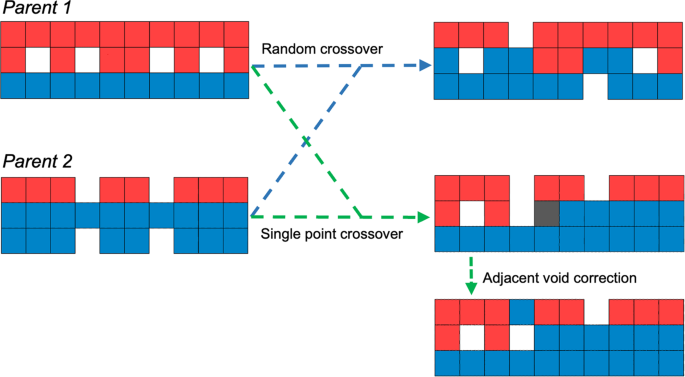
Every voxel has a 50–50 chance of inheriting the properties from either parent, and single point crossover where two children are produced from two parents with genome splicing at one point (represented here by the grey voxel).
-
Random crossover - Every voxel in the first child has a 50% chance of inheriting the value from parent 1 or parent 2. For example, if the first child obtains the value of the first voxel from parent 2, the second child automatically obtains the value from parent 1. This process is run for every voxel in the structure to obtain the new materials distributions.

As with the selection process, it is crucial to verify the positions of the void voxels in the children population. If there is a group of void elements that does not respect the set criteria, one is selected randomly and converted into an inert material (0→2). The children population is thus formed.
Mutation
The next stage is the mutation process, which occurs independent of the crossover process. In other words, an individual created by crossover can still be affected with a mutation. Mutations consist of minimal, local changes in the genome to inject diversity in the population. However, mutations are a special case where, to properly replicate the process that happens in nature, only the changes that produce better solutions with better fitness ‘survive’. Consequently, this requires an intermediate evaluation stage to recalculate the score of an individual after a mutation is applied. Since this is computationally expensive, the probability of a mutation happening is kept low. One of three mutation strategies can be employed as follows:
-
Apply active material: a randomly chosen voxel that is not made of an active material (0 or 2) is converted into an active material (1) (see Fig. 4a).
Fig. 4: The mutations are applied to the genome created from random crossover in Fig. 3. 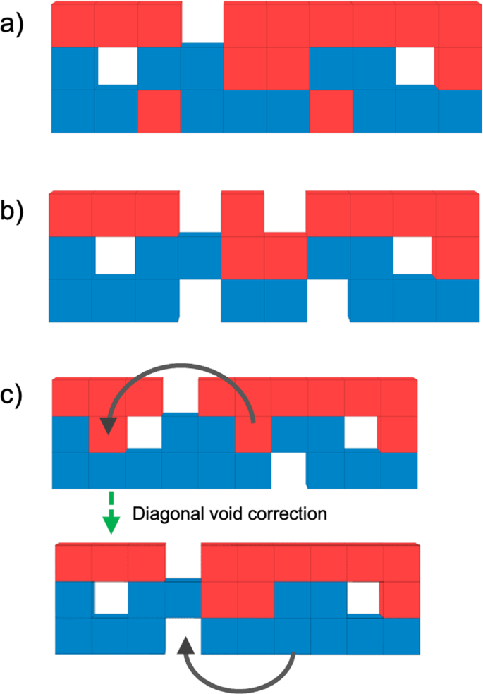
(a) two active material voxels replace a passive material and a void element, (b) two void elements replace an active and a passive material voxel, (c) a sequence shifting is applied and upon encountering a restriction, a different shift point is chosen.
-
Apply void: similarly, a randomly chosen voxel that is not a void element (1 or 2) is converted into one void (0) (see Fig. 4b).
-
Shift: a randomly chosen voxel is extracted and plugged into another randomly chosen point within the genome, the rest of the sequence is thus shifted one place to accommodate this (see Fig. 4c).

For the second and third operations, the position of void elements needs to be checked again to ensure that the void placement criterion is respected. Thus, each generated distribution will be verified and regenerated until a plausible mutation is created. The created mutation and its initial individual are both evaluated and compared to each other to ensure that the mutation yields better results. If this is not the case, a new mutation is generated and evaluated until a suitable mutation is achieved or the maximum number of mutation evaluations is reached, in which case the original unmutated individual is maintained.
The entire design process is illustrated in Fig. 5 where the user can input the parameters for the part creation, such as the dimensions and the materials used, and the target displacement, either by plugging in a target material distribution that is then evaluated to obtain the target displacements or by directly calculating the target displacements via mathematical equations.

By considering a voxel-based representation of a design space, the computational design process starts from a target shape (or displacement) and uses a FEA-based EA. It combines the advantages of optimizing both the materials distribution and material layout via TO to solve the inverse design problem of finding an optimal design to achieve a target shape by integrating void voxels.
Material models
It is crucial to use material models that sufficiently represent their real-world counterparts based on function without overloading the computational cost. A simple linear elastic model is used to characterize the inert material with the following mechanical properties: Young’s modulus E = 2.1 MPa and Poisson’s ratio ν = 0.3. As for the smart material, two choices are available: a liquid crystal elastomer and a hydrogel, both are sensitive to temperature.
Liquid Crystal Elastomer (LCE)
This active material is modelled as an incompressible thermoelastic solid with temperature-dependent thermal expansion behavior. An LCE part shrinks along its nematic direction, which refers to its printing (extrusion) direction, and expands following the other principal directions. In general, this behavior is achieved via direct ink writing where the mesogen alignment is controlled by both the ink extrusion and the nozzle path13. The contraction following the nematic direction is simulated using a negative coefficient of thermal expansion (CTE) while an anisotropic, or more specifically, a transversely isotropic expansion (non-uniform) is considered. The contractile thermal strain following this direction is thus characterized as eT and the strain following the directions perpendicular to the filament is characterized as \(\frac{{ - e_T}}{2}\). An equilibrium contraction is assumed such that the CTE values depend purely on the current temperature of the structure T and the reference temperature of the material Tref, where the thermal strain is null. This material constitutes the active material used in all the examples and case studies presented in this paper and represented in red voxels. For FEM simulations, each voxel was meshed with C3D8R elements in the commercial software ABAQUS. A linear elastic material is considered instead of a hyperelastic material as the latter is limited solely to isotropic thermal expansions in ABAQUS.
Hydrogel
A simplistic version of a temperature-sensitive hydrogel42,43 is modelled with an incompressible neo-Hookean material model such that the strain energy potential is defined as below:
where U is the strain energy per unit of reference volume, C10 and D1 are temperature-dependent material parameters, \(\bar I_1\) is the first deviatoric strain invariant defined as:
where the deviatoric stretches \(\bar \lambda _i\) is expressed as follows:
J is the total volume ratio, Jel is the elastic volume ratio, and λi are the principal stretches. The elastic volume ratio Jel relates the total volume ratio J and the thermal volume ratio Jth, as follows:
The thermal volume ratio Jth can be given by:
where εth is the linear thermal expansion strain that is obtained from the temperature and the isotropic CTE.
An incompressible model would give us the following simplification:
For FEM simulations in the ABAQUS software, hybrid C3D8RH elements were used.
Target shape from known target distribution
The first case study aims to gauge the efficacy of the framework by exploiting the option of setting the target shape via a known target distribution in a nonlinear inverse problem. A classic example of a cantilever beam that deforms into a parabola shape when subjected to a force exerted on its unrestrained extremity is emulated as it involves a known and intuitive material distribution in the context of design for 4D printing. A beam with dimensions (\(240\,{{{\mathrm{mm}}}} \times 30\,{{{\mathrm{mm}}}} \times 5\,{{{\mathrm{mm}}}}\)) is voxelized as illustrated in Fig. 6 and affected with the shown material distribution. It is interesting to note that, by limiting the target distribution to voxels consisting of smart and inert materials, a more controlled target shape is achieved while simultaneously examining the pertinence of adding void voxels. This, while serving as a benchmark test, can also be equated to a classic TO problem by imposing the use of void voxels and effectively reducing the amount of material used in the final design solution. The impact of adding void voxels on the active material fraction can also be observed.

In this voxel-based model, active material and passive material are distributed through red voxels and blue voxels, respectively.
The beam is fixed on the left end and an external temperature range of 40°C to 80°C is applied to achieve a large bending, with a reference temperature of -20°C. A deflection or total displacement of 76 mm following the y direction is observed, indicated in Fig. 7, which constitutes 31% of the total length of the structure, effectively placing this example in the realm of a nonlinear problem. The parameters used for the EA are shown in Table 1.

The beam—fixed on the left side—exhibits a large deflection (76 mm) once thermally stimulated (from 40 °C to 80 °C).
The result for the entire process is presented in Fig. 8. The convergence analysis, as illustrated in Fig. 8c, is represented by the fitness statistics, consisting of the minimum fitness corresponding to the best individual of the population and the average fitness of the entire population, which describes the overall performance of the population.

(a) the displacement of the optimal solution, (b) the optimal materials distribution generated by the EA, and (c) convergence statistics for the evolutionary process.
As shown in Table 1, a population size of 10 individuals is evolved for 25 generations, towards the end of which the fitness converged to a MSE of 0.5, which corresponds to a geometric agreement with approximately 7% error. The final deformed shape as well as the optimal material distribution is presented in Fig. 8a and b. A total of 250 FEM simulations were run for approximately 12 hours to obtain the results presented. The simulations were launched on a central processing unit (CPU) only setting (Intel(R) Xeon(R) CPU E5–1607 v4 @ 3.10 GHz) and without parallelization, which explains the length of the total duration of the process. Admittedly, a bigger population size and number of generations will yield better results and the possibility of utilizing a more powerful computer greatly reduces the computational cost of the entire process.
As shown in Table 1, the first population of generated individuals were constrained to a certain active material fraction and void fraction. These values are then allowed to evolve throughout the process via crossover and mutation. As a result, the optimal solution found consists of lesser material due to the incorporated void voxels and more specifically lesser active material (0.33–24 voxels in the target distribution vs 0.25–18 voxels in the optimal solution).
Target shape based on a Bezier curve
A standard employment of mathematical equations to find the target displacement values that is then plugged into the fitness function includes polynomial equations and multiperiodic sinusoidal equations. However, to maximize the capacity of the framework to solve for 2D shape changes, it is essential to introduce multivariable displacement equations. Since it is complicated to specify the target displacements in both directions, especially in the context of large deformations, a novel approach is adopted. A user-friendly method to design the target shape is via Bezier curves. Bezier curves are parametric curves that allows the user to define a smooth, continuous curve using discrete control points. Although these curves can be represented via specific functions, a more hands-on strategy is opted for, via a module designed on the graphical algorithm editor Grasshopper® (GH), an add-on of the commercial computer-aided design (CAD) software Rhinoceros© (RH).
As shown in Fig. 9, the user inputs the length of the structure as well as the coordinates of the control points. A Bezier curve is formed and then scaled down until the final length of the deformed structure is equivalent to the length of the initial, undeformed structure. Both the curves are then partitioned into equal segments with points that act as sample points. A vector cluster then describes the displacement of each of these points in the x and y directions, which serve as the target displacement values for the fitness function (Fig. 9). This one-dimensional representation of the deformed structure is replicated following the y-direction and then slightly scaled down following the x direction to achieve a two-dimensional equivalent of the target displacement values as shown in Fig. 9. Some of the simplifications employed to utilize this method include the hypothesis that the structure remains the same length after deformation and that the sample points remain equidistant from one another. As such, the second case study uses this method to set the target displacement. A beam with dimensions (\(240\,{{{\mathrm{mm}}}} \times 15\,{{{\mathrm{mm}}}} \times 2\,{{{\mathrm{mm}}}}\)) was used with a temperature-sensitive hydrogel (with a CTE equal to 0.001) as the active material. The beam is fixed on the left end and a temperature range of 40°C to 70°C is applied. The maximum target displacement in this example is equal to 17.5 mm.

(a) The component in GH used to generate and control the Bezier curves. (b) The generated Bezier curve (undeformed structure in blue, deformed structure in green, control points in red, displacement vectors in black). (c) The curve is stacked to provide a 2D representation.
The results for the second case study are presented in Fig. 10. The convergence analysis, as illustrated in Fig. 10c shows that the overall fitness of the population throughout the entire process remained relatively low compared to the first study due to the difference in the maximum displacement. The second case study has a much smaller maximum displacement to attain as the focus is towards achieving the more complex form. Thus, the MSE of each of the individuals in the second case logically cannot be higher than the first case. A population size of 10 individuals is evolved for 30 generations, towards the end of which the fitness converged to a MSE of 0.25. Similar to the first case, the maximum error was found near the region that is subjected to the maximum displacement and away from the fixed extremity. A total of 300 FEM simulations were thus ran for approximately 7 hours with the same computer configuration. The EA input parameters remained the same, however, due to the complexity of the form, a much higher active material fraction was required to achieve the shape change.

(a) the displacement of the optimal solution, (b) the optimal material distribution generated by the EA, and (c) convergence statistics for the evolutionary process.
The proposed FEA-EA approach incorporates the notion of TO via the incorporation of void elements in a standard EA process. The usage of an EA as opposed to other gradient-based methods allow us to simulate large-deformation, nonlinear problems with a voxel-based geometry which facilitates not only the definition of the geometry with discrete materials but also the inclusion of equally sized void elements. The inherent separation between the EA and the FEM simulations allows us to apply this method with vastly different material models, two of which are described and used in the problems above. However, one of the downsides of the EA method owes itself to its iterative strategy. In other words, the speed and accuracy of the process is largely dependent on the individuals generated in the beginning. A population of substandard individuals will also reduce the chances of finding the best solution possible and lead to a situation akin to a local minimum.
The case studies presented aim to showcase the two different methods of defining the target shape that is available in the framework. The first emulates a classic TO problem by introducing a fixed ratio of void voxels and active material in the beginning. The second case demonstrates an alternative method in design for 4D printing using Bezier curves whereby the target shape is defined manually via control points. This addition has decomplexified the usage of strictly mathematical representations of geometry and allows a layman to design. Moreover, in this specific context, using Bezier curves were necessary to properly identify the displacement of the structure in 2D after deformation.
The results shown in Figs. 8 and 10 demonstrate the effectiveness of the framework in finding an optimal solution for a given problem with decent agreement considering the number of simulations run to achieve the results. As mentioned above, better results can be expected with more computational power and the parallelization of the process in terms of simulations. Furthermore, with a lower computational cost, more complex problems can be incorporated with increasingly accurate constitutive material models.
In this paper, we present a framework based on the coupling of EA and FEM analysis in the design of active composite structures for 4D printing. The inclusion of void elements in the volumetric materials distribution of the generated solutions has allowed for an amalgamation of shape-matching algorithms with TO. We have presented two case studies with distinct methods to set the target shape as well as different smart material models that have yielded results with good agreement to the target shape. This approach is a start towards finding non-intuitive design solutions in more complex designs while minimizing the quantity of material required. Future advances for this approach include adapting the framework for three-dimensional (3D) design and solving more complex problems using machine learning techniques.
Method
The proposed computational framework has been implemented in a program written in Python 2.7 and adapted to be launched via ABAQUS CAE’s python scripting within the ABAQUS software and the settings and steps depend on the chosen active material. The program is structured into two principal classes, VoxAbaqus, that contains the methods used to run commands directly in ABAQUS, such as assigning material distributions to a structure or creating a material, and EvolutionaryAlgorithm which contains the methods that govern the EA processes, such as crossover and mutation. The latter class pilots and calls methods from the former class. The slightly outdated version of Python limits the number of libraries that can be imported and utilized.
Data availability
Data supporting the findings of this study are available from the corresponding author (FD) on reasonable request.
Code availability
Code supporting the findings of this study are available from the corresponding author (FD) on reasonable request.
References
Roach, D. J. et al. 4D printed multifunctional composites with cooling-rate mediated tunable shape morphing. Adv. Func. Mat. 32, 2203236 (2022).
Mao, Y. Q. et al. Sequential self-folding structures by 3D printed digital shape memory polymers. Sci. Rep. 5, 13616 (2015).
Zhao, Z. A., Kuang, X., Yuan, C., Qi, H. J. & Fang, D. N. Hydrophilic/hydrophobic composite shape-shifting structures. ACS Appl. Mater. Interfaces 10, 19932 (2018).
He, M. et al. Multi-material topology optimization of piezoelectric composite structures for energy harvesting. Composite Struct. 265, 113783 (2021).
Montgomery, S. M. et al. Magneto-mechanical metamaterials with widely tunable mechanical properties and acoustic bandgaps. Adv. Funct. Mater. 31, 2005319 (2020).
Sundaram, S., Skouras, M., Kim, D. S., van den Heuvel, L. & Matusik, W. Topology optimization and 3D-printing of multimaterial magnetic actuators and displays. Sci. Adv. 5, 1–43 (2019).
Lendlein, A., Jiang, H., Jünger, O. & Langer, R. Light-induced shape-memory polymers. Nature 434, 879–882 (2005).
Wu, J. et al. Multi-shape active composites by 3D printing of digital shape memory polymers. Sci. Rep. 6, 24224 (2016).
Alagha, A. N., Hussain, S. & Zaki, W. Additive manufacturing of shape memory alloys: A review with emphasis on powder bed systems. Mater. Des. 204, 109654 (2021).
Yuan, C. et al. 3D printed reversible shape changing soft actuators assisted by liquid crystal elastomers. Soft Matter 13, 5558–5568 (2017).
Roach, D. J. et al. Novel ink for ambient condition printing of liquid crystal elastomers for 4D printing. Smart Mater. Struct. 27, 125011 (2018).
Roach, D. J. et al. Long liquid crystal elastomer fibers with large reversible actuation strains for smart textiles and artificial muscles. ACS Appl. Mater. Interfaces 11, 19514–19521 (2019).
Peng, X. et al. 4D printing of freestanding liquid crystal elastomers via hybrid additive manufacturing. Adv. Mater. 34, 2204890 (2022).
Chester, S. A. & Anand, L. A thermo-mechanically coupled theory for fluid permeation in elastomeric materials: Application to thermally responsive gels. J. Mech. Phys. Solids 59, 1978–2006 (2011).
Toh, W. et al. Mechanics of inhomogeneous large deformation of photo-thermal sensitive hydrogels. Int. J. Solids Struct. 51, 4440–4445 (2014).
Demoly, F., André, J. C. 4D printing Volume 1: Between disruptive research and industrial applications (Wiley-ISTE, London, 2022).
Demoly, F., André, J. C. 4D printing Volume 2: Between science and technology (Wiley-ISTE, London, 2022).
Dimassi, S. et al. An ontology-based framework to formalize and represent 4D printing knowledge in design. Computers Ind. 126, 103374 (2021).
Demoly, F., Dunn, M. L., Wood, K. L., Qi, H. J. & André, J. C. The status, barriers, challenges, and future in design for 4D printing. Mater. Des. 212, 110193 (2021).
Ly, S. T. & Kim, J. Y. 4D printing – fused deposition modeling printing with thermal-responsive shape memory polymers. Int. J. Precis. Eng. Manuf. – Green. Technol. 4, 267–272 (2017).
Lewis, J. A. Direct ink writing of 3D functional materials. Adv. Funct. Mater. 16, 2193–2204 (2006).
Gladman, A. S., Matsumoto, E. A., Nuzzo, R. G., Mahadevan, L. & Lewis, J. A. Biomimetic 4D printing. Nat. Mater. 15, 413 (2016).
Armstrong, C. D., Yue, L., Deng, Y. & Qi, H. J. Enabling direct ink write edible 3D printing of food purees with cellulose nanocrystals. J. Food Eng. 330, 111086 (2022).
Li, V. C. F., Dunn, C. K., Zhang, Z., Deng, Y. & Qi, H. J. Direct ink write (DIW) 3D printed cellulose nanocrystal aerogel structures. Sci. Rep. 7, 8018 (2017).
Fu, Q., Saiz, E. & Tomsia, A. P. Direct ink writing of highly porous and strong glass scaffolds for load-bearing bone defects repair and regeneration. Acta Biomaterialia 7, 3547–3554 (2011).
Ge, Q., Qi, H. J. & Dunn, M. L. Active materials by four dimensions printing. Appl. Phys. Lett. 103, 131901 (2013).
Khondoker, M. A. H., Baheri, N. & Sameoto, D. Tendon-driven functionally gradient soft robotic gripper 3D printed with intermixed extrudate of hard and soft thermoplastics. 3D Print. Addit. Manuf. 6, 191–203 (2019).
Kim, B. et al. Rapid custom prototyping of soft poroelastic biosensor for simultaneous epicardial recording and imaging. Nat. Commun. 12, 3710 (2021).
Zolfagharian, A., Denk, M., Bodaghi, M., Kouzani, A. Z. & Kaynak, A. Topology-optimized 4D printing of a soft actuator. Acta Mech. Solid. Sin. 33, 418 (2020).
Mitchell, A., Lafont, U., Holnska, M. & Semprimoschnig, C. Additive manufacturing – A review of 4D printing and future applications. Addit. Manuf. 24, 606–626 (2018).
Maute, K. et al. Level set topology optimization of printed active composites. J. Mech. Des. 137, 111402 (2015).
Jiang, W. et al. A voxel-based method of multiscale mechanical property optimization for the design of graded TPMS structures. Mater. Des. 204, 109655 (2021).
Tang, D., Hao, L., Li, Y., Li, Z. & Dadbakhsh, S. Dual gradient direct ink writing for formation of kaolinite ceramic functionally graded materials. J. Alloy. Compd. 814, 152275 (2020).
Fernandes, P., Guedes, J. M. & Rodrigues, H. Topology optimization of three dimensional linear elastic structures with a constraint on “perimeter”. Computers Struct. 73, 583–594 (1999).
Zhu, B., Skouras, M., Chen, D. & Matusik, W. Two-Scale topology optimization with microstructures. ACM Trans. Graph. 36, 120b (2017).
Sossou, G. et al. Design for 4D printing: A voxel-based modeling and simulation of smart materials. Mater. Des. 175, 107798 (2019).
Sossou, G. et al. Design for 4D printing: Modeling and computation of smart materials distributions. Mater. Des. 181, 108074 (2019).
Benyahia, K. et al. A computational design approach for multi-material 4D printing based on interlocking blocks assembly. Addit. Manuf. 58, 102993 (2022).
Langley, P. The changing science of machine learning. Mach. Learn. 82, 275–279 (2011).
Salonitis, K., Chantzis, D. & Kappatos, V. A hybrid finite element analysis and evolutionary computation method for the design of lightweight lattice components with optimized strut diameter. Int. J. Adv. Manuf. Tech. 90, 2689–2701 (2017).
Abdi, M., Wildman, R. & Ashcroft, I. Evolutionary topology optimization using the extended finite element method and isolines. Eng. Optim. 46, 628–647 (2014).
Hamel, C. M. et al. Machine-learning based design of active composites for 4D printing. Smart Mater. Struct. 28, 065005 (2019).
Sun, X. et al. Machine learning-evolutionary algorithm enabled design for 4D-printed active composite structures. Adv. Funct. Mater. 32, 2109805 (2021).
Acknowledgements
The research work is part of a much larger project in the field of design for 4D printing. The authors would like to thank the French ‘Investissements d’Avenir’ program, project ISITE-BFC 4D-META (contract ANR-15-IDEX-0003) as the main financial support of this research activity, the EIPHI Graduate School (contract ANR-17-EURE-0002), and the S.mart academic society for their contribution.
Author information
Authors and Affiliations
Contributions
D.A.: Conceptualization, Methodology, Writing – original draft, Software. R.P.: Conceptualization, Software. D.C.: Methodology, Writing – review & editing. H.J.Q.: Methodology, Writing – review & editing. M.B.: Writing – review & editing. J-C.A.: Writing – review & editing. F.D.: Conceptualization, Methodology, Supervision, Funding acquisition, Writing – review & editing.
Corresponding author
Ethics declarations
Competing interests
The authors declare that they have no known competing financial interests or personal relationships that could have appeared to influence the work reported in this paper.
Additional information
Publisher’s note Springer Nature remains neutral with regard to jurisdictional claims in published maps and institutional affiliations.
Rights and permissions
Open Access This article is licensed under a Creative Commons Attribution 4.0 International License, which permits use, sharing, adaptation, distribution and reproduction in any medium or format, as long as you give appropriate credit to the original author(s) and the source, provide a link to the Creative Commons license, and indicate if changes were made. The images or other third party material in this article are included in the article’s Creative Commons license, unless indicated otherwise in a credit line to the material. If material is not included in the article’s Creative Commons license and your intended use is not permitted by statutory regulation or exceeds the permitted use, you will need to obtain permission directly from the copyright holder. To view a copy of this license, visit http://creativecommons.org/licenses/by/4.0/.
About this article

Cite this article
Athinarayanarao, D., Prod’hon, R., Chamoret, D. et al. Computational design for 4D printing of topology optimized multi-material active composites. npj Comput Mater 9, 1 (2023). https://doi.org/10.1038/s41524-022-00962-w
Received:
Accepted:
Published:
DOI: https://doi.org/10.1038/s41524-022-00962-w
This article is cited by
-
Application of self-supervised approaches to the classification of X-ray diffraction spectra during phase transitions
Scientific Reports (2023)
-
Accurate energy barriers for catalytic reaction pathways: an automatic training protocol for machine learning force fields
npj Computational Materials (2023)
