
Abstract
Tailings dams retain the waste by-products of mining operations and are among the world’s largest engineered structures. Recent tailings dam failures highlight important gaps in current monitoring methods. Here we demonstrate how ambient noise interferometry can be applied to monitor dam performance at an active tailings dam using a geophone array. Seismic velocity changes of less than 1% correlate strongly with water level changes at the adjacent tailings pond. We implement a power-law relationship between effective stress and shear wave velocity, using the pond level recordings with shear wave velocity profiles obtained from cone penetration tests to model changes in shear wave velocities. The resulting one-dimensional model shows good agreement with the seismic velocity changes. As shear wave velocity provides a direct measure of soil stiffness and can be used to infer numerous other geotechnical design parameters, this method provides important advances in understanding changes in dam performance over time.
Introduction
Global demand for minerals is rising, with additional pressure on supply driven by the transition to renewable energy sources1,2. Alongside declining ore grades, this demand is increasing the volume of waste material, known as tailings, produced by the mining industry3,4. Tailings dams, designed to retain the waste by-products of mining, are among some of the largest engineered structures in the world5; there are an estimated 8100 tailings facilities worldwide4. Tailings dams are designed and constructed under similar regulations as conventional water storage dams in many industrialized nations6. However, the likelihood of tailings dam failures is approximately two orders of magnitude higher, and the risk of future tailings dam failures is projected to increase2,5. The 2019 Brumadinho, Brazil tailings dam failure caused over 270 deaths, was an environmental disaster, and increased public scrutiny of tailings dams worldwide4,7,8. Forensic investigations of the failure classified it as a flow liquefaction event and indicated that none of the monitoring instrumentation installed (which included piezometers, inclinometers, survey markers, flow meters, and rain gauges) was able to detect any notable changes prior to the failure. Furthermore, the investigations also indicated that the deformations obtained using post-failure satellite remote sensing (interferometric synthetic aperture radar) analysis were consistent with ongoing internal creep, and were not considered a precursor to failure9. This failure illustrates the challenges of designing and maintaining a tailings dam monitoring system capable of providing adequate lead time up to a failure. Despite this, the majority (94%) of tailings dam practitioners surveyed in a 2019 study2 felt that their site represented industry best practice for tailings dam monitoring. An earlier review on the state of practice for tailings dam monitoring identified extensive gaps, including the use of outdated point-based sensors and insufficient redundancy of sensors10. To address these gaps, the authors’ recommendations included combining point-based sensors with broad area measurements. Remote sensing methods are broad area measurements that are increasingly being used to support tailings dam monitoring7,11,12,13,14 by detecting changes at surface. Alternatively, geophysical-based monitoring methods detect changes in the subsurface that aren’t measurable using remote sensing methods15,16,17,18,19. Ambient noise interferometry (ANI) is a geophysical technique that relies on the reconstruction of the impulse response of a wavefield by cross-correlating the naturally occurring noise signals between a pair of seismic sensors, where one acts as a virtual source and the other as a receiver20,21. The wavefield includes coda waves in the later portion of the seismogram. Coda waves represent scattered waves that have spent more time propagating within the medium, and are more sensitive to seismic velocity changes20,22. By monitoring temporal changes in the coda portion of the wavefield propagating between the sensors, relative changes in seismic velocities are measured, commonly referred to as dv/v. This method has been used to monitor volcanoes, landslides, and dams23,24,25,26,27, but is not yet an established technique for tailings dam monitoring.
Shear wave velocities (Vs) are an important parameter for evaluating the liquefaction susceptibility of tailings materials28,29. Industry standard methods for obtaining Vs for liquefaction assessments include in-situ measurements with seismic cone penetration testing (sCPT), geophysical methods such as multi-channel and spectral analysis of surface waves, seismic refraction tomography, downhole and crosshole tests, and laboratory measurements using bender elements or resonant column tests30. These methods are generally used to characterize site conditions at one point in space and time, as multiple acquisitions are costly and time-consuming. As coda waves are highly sensitive to Vs20, ANI could become an important component for tailings dam monitoring applications, by improving understanding of how Vs may change over time.
Results
Seismic velocity changes and environmental site data
We employ ANI using a geophone array at a mine site in northern Canada, located within a relatively aseismic region. Mine tailings at the site are hydraulically transported via pipeline and are deposited into a tailings beach adjacent to the dam (Fig. 1). The tailings dam is approximately 8 m in height and is constructed using the upstream method31. The dam is primarily comprised of compacted tailings materials, and hydraulically placed coarse tailings material are present where the geophone array extends into the tailings beach. The tailings are non-plastic, and gradation generally varies from a fine sandy silt to silty sand material. A generalized stratigraphic cross-section of the dam shows that the compacted tailings was originally placed over hydraulically placed tailings material (Fig. 1d). A tailings pond is located ~200 m to the north of the geophone array (Fig. 1a). Pond levels fluctuated throughout the data acquisition period and are controlled both by environmental (e.g., rainfall, seasonal changes in groundwater levels) and operational factors (e.g., variable pumping rates). Further details on the environmental site data are available in Supplementary Notes 1. We acquired vertical-component waveform data from twenty-five 5 Hz geophones in a T-shaped array during active and inactive construction periods, from June to early August 2020 (Fig. 1). The array geometry configuration, with 19 geophones along the dam crest and 6 geophones extending into the tailings beach, was selected to optimize the noise sources around the site and to avoid nearby construction downstream of the dam (see Methods). As ANI requires coherent cross-correlation waveforms and the active construction period resulted in incoherencies, these were removed from the dataset and only inactive construction period seismic data (three hours recorded per day) were relied on for further processing (Fig. 2).

a Geophone array overlain on lidar data with hill shading (1 m contours, collected in November 2020). Map was created using Global Mapper v21.0 software. Location of subset of sCPTs used in regression analyses. Additional sCPTs used in analyses are not shown as they are outside of the figure extents. b Twenty-five geophone array (20 on dam crest, five on tailings beach), showing cross-section A-A′. c Cross-section A-A′ of the tailings dam. The dashed black line shows approximation of dam fill and tailings extent for an upstream tailings facility, and does not represent actual delineated extents of fill and tailings. d Site stratigraphy obtained from historical borehole information.

a Spectral frequency content for a single station on one day of data acquisition for active and inactive construction periods. b Daily cross-correlations over data acquisition period for a single station pair. The lower graph shows the stacked (reference cross-correlation) waveform of individual daily cross-correlations over the data acquisition period.
Standard ANI processing methodologies were applied to obtain seismic velocity changes (dv/v) (see Methods). The dv/v estimates were compared with other site information, including: tailings pond levels, daily rainfall, atmospheric pressures and temperature data. During the monitoring period, three main trends are observed: (1) a dv/v increase of ~0.6% over the first month of recording coincides with decreasing water levels at the pond; (2) a dv/v decrease >0.5% in the five days following the highest daily rainfall during the monitoring period; and (3) a dv/v recovery to the pre-rainfall levels in the final week of data acquisition (Fig. 3).

Average dv/v over the geophone array is plotted as a thick black line, with minimum and maximum extents of individual virtual sources averaged over all receiver combinations shaded in light gray. The nearby pond elevation is plotted on the same graph with an inverted y-axis, to illustrate the inverse correlation of the pond levels with dv/v. Three main trends are observed: a an increase in dv/v of up to ~0.6% over the first month of data acquisition coincides with a decrease in water levels at the nearby pond, shown in yellow shading; b a decrease in dv/v of over ~0.5% in the five-days following the highest daily rainfall observed over the monitoring period, shown in pink shading; and c a recovery in dv/v to the pre-rainfall levels in the final week of data acquisition, shown in blue shading.
Effective stress model
The shear wave velocity (Vs) is an important parameter for geotechnical monitoring as it provides a direct measure of soil stiffness and can be used to infer numerous other geotechnical design parameters such as the stress state, liquefaction resistance and degree of cementation28,30,32. For a Poisson medium, Snieder20 demonstrated the higher sensitivity of the coda waves to Vs. Here, we provide evidence of this Vs sensitivity at a mine site in northern Canada, which can enable meaningful dam performance monitoring.
We modeled relative changes in Vs, (dVs/Vs) to validate our dv/v estimates by implementing a power-law relationship between Vs and effective vertical stress for granular materials (e.g., soils)33. This relationship applies under one-dimensional loading and vertical shear wave propagation direction34,35,36,37. Using the sCPT, the shear wave can be approximated as propagating vertically as it travels from the source at surface to the receiver at depth (within the cone)38. Thus, for effective vertical stress, Vs is represented as
where α and β represent material constants, and \({\sigma }_{v}^{{\prime} }\) is the effective vertical stress39,40. The material constant α represents the shear wave velocity at \({\sigma }_{v}^{{\prime} }\) equal to 1 kPa, and β is a measure of the stress-level dependency to shear waves and incorporates both interparticle contact behavior and fabric changes41. We obtained site-specific α and β parameters for the various stratigraphic units by performing a power-law regression analyses with bootstrap sampling, using Vs and \({\sigma }_{v}^{{\prime} }\) data obtained from 52 sCPTs completed in 2017 and 2018 (Fig. 4; Table 1). Power-law regression analyses, undertaken for the compacted tailings and glaciolacustrine clay unit, are shown in Fig. 5. Additional details of statistical analyses are described in Methods.

a Estimation of site specific α and β from power-law regression using Vs estimates from sCPT surveys and effective vertical stress for underlying tailings material. Bootstrap analyses, shown in shaded gray, were used to obtain 95% confidence intervals of the α and β parameters. Regression results for compacted/coarse tailings and clay units are presented in Fig. 5. b Modeled dVs/Vs based on α and β obtained from power-law regression for an optimized depth z in blue. Shaded blue area represents the maximum and minimum extents of 50,000 Monte Carlo simulations, and the blue line is the mean of all simulations. Average dv/v estimates over geophone array are shown as a black line, with gray shading representing maximum and minimum extents of individual virtual sources averaged over all receiver combinations. The average correlation coefficient, plotted as a marker, shown between the reference correlation waveform and the stretched waveform.

a Estimation of site specific α and β from power-law regression using Vs estimates from sCPT surveys and effective vertical stress for compacted and coarse tailings (upper plot) and glaciolacustrine clay (lower plot) materials. Bootstrap analyses, shown in shaded gray, were used to obtain 95% confidence intervals of the α and β parameters. b Probability density functions of the optimal depth z to minimize L1 misfit between dv/v estimates with dVs/dVs. Results obtained using bootstrap sampling (150,000 samples) followed by 50,000 iterations of Monte Carlo analyses. 95% confidence intervals are shown as black vertical lines.
Estimates of daily effective vertical stresses were inferred from daily resampled pond data using Eq. (6). These estimates, alongside site-specific α and β parameters (Table 1) were input into Eq. (1) to obtain daily Vs.
Relative changes in daily Vs were obtained, treating depths z as an unknown and varying it from near surface to bedrock depths (~39 m), using
where \(\bar{\,{{{{{{\rm{V}}}}}}}_{{{{{{\rm{s}}}}}}}}\) is the mean of all daily Vs estimates obtained with Eq. (1). The L1 norm was computed fitting the dVs/Vs prediction to the dv/v results. A grid search over z produced a minimum misfit for z equal to 15.7 m (Fig. 5b). Bootstrap analyses followed by Monte Carlo sampling were used to estimate uncertainties of the depth z obtained, with 95% confidence intervals from 14.1 m to 17.4 m (see Methods for details).
Figure 4 shows the predicted dVs/Vs results from the effective-stress model for the optimal z and dv/v results from ANI. The close agreement illustrates that the model successfully explains the ANI results to be predominantly changes in Vs, and that changes are primarily occurring at a depth of ~16 m. This primary sensitivity to shear waves is in agreement with the theoretical results for a Poisson medium20. Importantly, dominant sensitivity to Vs permits ANI results to be interpreted in terms of dam performance.
Discussion
Based on the general agreement between the dv/v measurements and the dVs/Vs model, our results demonstrate how ANI can be applied at a tailings dam site to provide highly sensitive (<1%) measurements of in-situ changes of Vs alongside an approximation of depth sensitivity, without requiring advanced geomechanical models. Our dv/v measurements suggest that effective stress changes have the strongest influence on dv/v, with our effective stress model replicating the three main trends visible in the dv/v curve (Fig. 3). However, some discrepancies remain. Our modeled dVs/Vs relies on an important assumption, that relative changes in pore pressure u near the tailings dam are attributed to the changes in the water levels recorded at the tailings pond. This was required considering the lack of available instrumentation recording pore pressure data over the geophone data acquisition period near our array. However, factors such as hydraulic conductivities and beach width, will contribute to variations in pore pressure between the tailings dam and the pond31, which could lead to discrepancies between our model and the dv/v observations. The effects of suction in the unsaturated zone are also neglected; thereby assuming the soil behaves either fully saturated below the inferred ground water level or fully unsaturated, above the inferred ground water level. Capillary forces in unsaturated soils contribute to an increase in the low strain stiffness, resulting in higher Vs in unsaturated versus saturated soils42. Future studies using this approach should attempt to locate the geophone array alongside instrumentation to monitor pore pressures (e.g., a piezometer) and suction (e.g., a tensiometer). This would help to improve understanding of the sensitivity of dv/v measurements to suction in the partially saturated zone, by comparing with a refined dVs/Vs model incorporating unsaturated soil mechanics.
Further discrepancies are notable when observing the higher variability in the dv/v traces, particularly from July 15 to 17, 2020 (Fig. 3). We attribute this variability to nearby construction at the south of the geophone array, resulting in lower waveform coherencies over these periods. This underlines a general limitation of applying ambient noise interferometry for monitoring, as changes in noise characteristics at the site could affect the quality of the estimated seismic velocity changes18. To account for potential apparent velocity changes attributable to changes in noise characteristics and not changes in dam performance, the stability of the noise sources used for dv/v monitoring should be reviewed on an ongoing basis (e.g., via power spectral density plots as shown in Fig. 2a).
We attribute our lack of meaningful correlations between dv/v and temperature or barometric pressure data to the shorter seismic data acquisition period (~41 days) over summer, preventing us from observing seasonal changes in dv/v, as observed by others18,43,44. The effects of barometric pressure were also neglected within our effective stress model, considering the non-linearity of barometric pressures at depth (e.g., damping and time delay effects), dependent on soil properties and groundwater levels45.
We developed an effective approach to apply effective stress principles46 to model dVs/Vs in the near surface. An alternative approach47 relies on physics-based modeling to demonstrate that changes in shear wave velocities are primarily caused by fluctuations in effective stress. Modeled changes in seismic surface wave velocity were obtained using relationships applicable to deeper structures in the order of hundreds of meters, using a spectral element method48. In comparison, our model is catered towards near surface applications in soils and fractured rock41, as it is based on the empirical equations shown in Eq. (6), using fundamental principles of soil mechanics. Our approach is desirable for tailings dams monitoring applications, since site-specific sCPT data are typically available and our stress model requires lesser computing power in comparison to alternative numerical modeling techniques.
In addition to providing an estimate of Vs changes for comparison with dv/v, our effective stress model provides information on the range of depths at which the dv/v are most likely to occur. Our model estimates a maximum depth sensitivity near ~16 m. We obtain an independent estimate, using the average wave speeds of the medium and the range of frequencies used in the analysis. The depth sensitivity of the dv/v estimates is dependent on the frequency band applied to the cross-correlations (5 to 15 Hz in this work). In an isotropic and homogeneous medium, most of the Rayleigh-wave energy at a frequency f is contained from surface to a depth z at approximately one third of a wavelength λ49. The average Vs in the dam fill (compacted tailings) and underlying tailings can be approximated as 300 m/s and 200 m/s, respectively, based on nearby sCPTs. As such, we estimate an average Vs of ~220 m/s over the topmost 39 m (i.e., from surface to bedrock) near our geophone array. Assuming a homogeneous medium, wavelengths for this Vs are between 15 m and 44 m, which suggest depth sensitivity between 5 m and 15 m. This is within reasonable approximation of our modeled depth sensitivity of ~16 m, considering the inhomogeneity of the structure (with a higher-velocity dam fill layer overlying lower-velocity tailings).
An important consideration of any tailings dam monitoring method, is its ability to detect pre-cursors leading up to a tailings dam failure. Tailings dams fail due to a variety of causes, such as overtopping, structural and foundation conditions, seismic instability, seepage and internal/external erosion50. As ANI is highly sensitive to changes in Vs which can be used as a proxy for soil stiffness, it provides important information leading up to a potential tailings dam failure. Although our dataset does not capture a failure occurring, a laboratory-scale experiment of an embankment dam undergoing failure due to internal erosion (i.e., piping) demonstrates that ambient noise methods are capable of detecting potential causes of tailings dam failures24. In this experiment, seismic velocity decreases of up to 20% were observed, which were attributed to stress redistribution as piping progressed. Our approach averages the dv/v over all geophone pairs with spacing ranging from 10 m to 180 m, thereby providing an estimated average change in Vs over a wider areal extent at the location of the geophone array (Fig. 1). It should be noted that the spatial resolution of this method is site-dependent, as it depends on the frequency content of the ambient noise generated, as well as the velocity structure at the site. Therefore, some mine sites may have increased spatial resolution (and vice versa). Regardless, this method could be used to alert to potential areas of concern by establishing a trigger threshold level based on seasonal fluctuations. For example, a ±2.5% threshold was used to monitor the Pont Bourquin landslide for five years with no false alerts26. At this same site, pre-cursory changes in seismic velocities of up to 7% in the days leading up to a flow-type failure were detected by applying similar ambient noise techniques25. As Vs measurements are used in the evaluation of the liquefaction resistance of a soil28, combining modeled dVs/Vs with ANI could inform on changes in liquefaction potential of the in-situ tailings material and underlying foundation. For instance, as liquefaction involves a phase-change in the medium from a solid to liquid state, it follows that the Vs will also decrease dramatically51. Further research of liquefaction-type failures is needed to improve understanding of whether adequate warning time could be provided by monitoring changes in Vs52.
The α and β parameters, obtained using Vs from sCPTs or from other means (e.g., multichannel analysis of surface waves), are of key importance to inform our dVs/Vs model and to provide further characterization of the stratigraphic units. However, the uncertainties of the α and β parameters vary considerably depending on the unit. Lower uncertainties correspond to the tailings unit, with increasing uncertainties for the clay and compacted/coarse tailings units (Fig. 5). This is attributed to an overall lower number of samples and the heterogeneity of these layers. Heterogeneity, such as increased cobbles or gravel, as well as higher resistance, due to compaction of the compacted tailings, prevents advancement of the sCPT, lowering the reliability of measurements obtained through these layers. Despite the higher uncertainties within the compacted/coarse tailings unit, the mean α, β values obtained are consistent with expected values for material undergoing cementation. For these material types, the Vs remains relatively consistent regardless of changes in stress, with β values approaching zero36. Cemented soils behave differently from non-cemented soils at both small and large strains, and are challenging to study in the laboratory setting due to sample preparation53. These findings illustrate how the α, β values can be a useful addition by providing complementary information that supports characterization of tailings, in addition to parametrizing the dVs/Vs model.
In conclusion, we developed an effective approach to advance tailings dam performance monitoring by combining ANI with a stress model calibrated with using tailings pond levels and sCPT data. Active mine sites are prime locations to study emerging monitoring methods such as ANI, as complementary site information (e.g., sCPTs, historical boreholes, weather station data), can be used to compare and validate results. As sCPTs are routinely carried out at many mine sites to assess the liquefaction potential of tailings, incorporation of sCPT data for model constraint allows for site-specific adaptation by mining practitioners. The data processing steps described do not require high computing power, and could be used to efficiently process incoming data for ongoing monitoring purposes. For example, in an operational setting, geophone data could be processed using a three-day rolling average to reduce errors and limit uncertainties18. Although the present study focuses on a relatively short (~180 m) segment of a tailings dam, the geometry of the geophone array can be adjusted by incorporating additional geophones as required to monitor along greater linear extents. An optimal segment length over which to average the dv/v should be carefully selected, considering the trade-off between spatial resolution and signal to noise ratio. Considering the current limited spatial resolution of this method, complementary monitoring techniques such as piezometers (e.g., pore pressures), interferometric synthetic aperture radar (e.g., surficial deformation) and slope inclinometers (e.g., lateral deformation) should be incorporated into an overall tailings dam monitoring system, rather than relying solely on this method. Although some open questions remain, the advances presented in this manuscript show the potential to use ANI as a quantitative real-time tool and increase our understanding of the temporal evolution of the internal state of tailings dams.
Methods
Seismic recordings and cross-correlations
Nineteen geophones were installed in a northwest-southeast orientation along the tailings dam crest and six were installed in a northeast to southwest orientation extending into the tailings beach. The maximum and minimum interstation distances were 180 m and 10 m, respectively. This array configuration was chosen in consideration of the average wave velocities in the upper 30 m of the site (~220 m/s) and to account for uncertainties surrounding directionality of the noise sources. Due to ongoing construction, it was unfeasible to install geophones along the dam slope and near the dam toe, although this would have been desirable from a monitoring perspective. Geophones were buried five to ten centimeters below ground to reduce the near surface effects of atmospheric pressure and temperature fluctuations. Geophones recorded for a 12-hour period per day. Nine hours of data were collected during active construction at the site, and three hours of data were collected when construction was not active. The ambient noise recorded during active construction was highly directive and sources moved in time and space, resulting in incoherent cross-correlation waveforms. Therefore, cross-correlations are only considered from recording times without construction, three hours per day (00:00 to 03:00 UTC; Fig. 2a).
Seismic data pre-processing included detrending, tapering, filtering and normalization54. The theory of ambient noise interferometry (ANI) assumes an isotropic and uniform noise source21,55. These theoretical requirements are typically not met; however, these conditions can be simulated by applying standard data processing methodologies54. Seismic data processing steps applied to the acquired seismic noise data are as follows:
-
1.
Raw Data Acquisition: Raw data were acquired at a sampling rate of 500 Hertz, collected over a 35 to 41 day period (dependent on battery life), from 15:00 to 03:00 UTC.
-
2.
Pre-processing: Data pre-processing included trimming, detrending, tapering, filtering and normalization:
-
Trimming: Data were trimmed to only include inactive construction periods (assumed to occur from 00:00 UTC to 03:00 UTC, based on construction schedule).
-
Detrending: Removal of linear trends.
-
Tapering: Taper the edges of the signal in preparation for filtering.
-
Filtering: Apply a bandpass filter from 5 to 15 Hz.
-
Time-domain normalization: One-bit normalization reduces the effect of instrumental irregularities, earthquake signals and non-stationary noise sources54.
-
Spectral whitening: Also known as frequency-domain normalization, spectral whitening broadens the frequency band of ambient noise and reduces the effect of monochromatic noise sources54.
-
-
3.
Cross-correlations: Each station pair combination (representing a virtual source and receiver) was cross-correlated using 20-s time windows with no overlap applied between windows. These windows were stacked to obtain daily cross-correlation waveforms. A reference cross-correlation waveform (required for monitoring seismic velocity changes) was obtained by stacking over the entire data acquisition period (35 to 41 days depending on the battery life of the geophone).
-
4.
Monitoring with ambient noise (dv/v): Relative changes in seismic velocities using the reference and daily cross-correlation waveforms are obtained using the ‘stretching’ method, by modifying the time axis using different seismic velocity changes23,56,57,58 (Fig. 6). The stretching methodology was applied to causal and acausal coda windows (±0.5 seconds to ±3.5 s, selected based on interstation spacing and visual inspection of waveform coherency) to obtain dv/v measurements, and causal and acausal windows were averaged to improve signal to noise ratio.
Fig. 6: Schematic showing the seismic data processing steps applied. 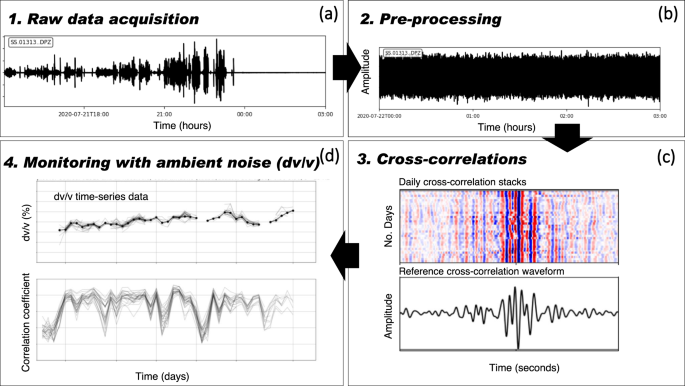
a Initial raw data acquisition includes both active and inactive construction periods. b Pre-processing described in Section 4, includes trimming, one-bit normalization and spectral whitening. c Daily cross-correlations are plotted as an image in the upper plot, with a reference cross-correlation shown below. d The dv/v time series data is obtained using a ‘stretching’ algorithm (upper plot), which also outputs a correlation coefficient representing the similarity between the daily waveform and reference waveform (lower plot).

Effective stress model
Shear wave velocities (Vs) were obtained approximately every meter along the sCPT profile by laterally striking a beam held in place by a normal load, using a sledgehammer38. Using a straight ray-path assumption, average Vs are ~300 m/s in the compacted tailings material and ~200 m/s in the tailings and underlying material, up until refusal. A generalized stratigraphy model based on historical borehole data is shown in Fig. 1d.
The velocity of shear waves traveling within a soil depends on the effective confining stress, saturation, and mass density36. For a homogeneous and isotropic medium, Vs can be expressed as a function of the small strain shear modulus (Gmax) and the bulk density of the soil (ρ),
The principle of effective stress46 defines the stress experienced by the soil skeleton that controls deformation. In a one-dimensional model, the effective vertical confining stress is equal to the overburden stress minus the pore pressure
where \({\sigma }_{v}\) is the total vertical stress and the pore pressure u is obtained from
where \({\gamma }_{w}\) is the unit weight of water (9.81 kN/m3) and \({d}_{w}\) is the depth to the inferred groundwater level, relative to the dam crest elevation. In Eq. (4), \({\sigma }_{v}\) can be approximated as the sum of the unit weights of each layer, multiplied by the thickness of that layer. Using the resampled daily pond data, we estimate \({\sigma }_{v}^{{\prime} }\) at depths varying from 1 m below surface to the approximate bedrock depth at 39 m at 0.1 m intervals, for each day. Equations to obtain the total vertical stress \({\sigma }_{v}\) for z in each layer, relative to the dam crest, are
where dw is the depth to the inferred groundwater level, h1 is the distance from surface to the dam fill and tailings boundary, and h2 is the distance from surface to the tailings and clay boundary (Fig. 1d). Unit weights are shown as γdf and γdf,sat, representing the moist and saturated compacted tailings (dam fill), γt,sat, representing the underlying tailings, and γGLU,sat representing the underlying glaciolacustrine clay unit.
Bootstrap analyses were performed on α and β parameters obtained from the power regression analyses, on the three units (compacted/coarse tailings, underlying tailings, clay). Initial α and β parameters were obtained by performing a power law regression on the dataset (corresponding to the scattered Vs/σv’ data from sCPTs). Using the initial α and β parameters with Eq. (1), a power-law dataset is reconstructed (representing the red dotted line in Fig. 4a). Then, for each bootstrap simulation (150,000 total), the dataset was randomly resampled with a uniform distribution, using the same size as the original dataset. Bootstrapped α and β parameters were then obtained using the power law regression for each simulation, and were each appended to an array to view their corresponding probability distributions (Fig. 7).

Bootstrap sampling (150,000 samples) for each unit (compacted and coarse tailings, fine tailings and glaciolacustrine clay) was completed to obtain probability density functions of the α and β parameters. Black vertical lines are used to indicate the 95% confidence intervals.
Monte Carlo simulations were then performed (50,000 iterations) to randomly select, using a uniform distribution, from the empirical cumulative distribution function of the α, β parameters obtained from bootstrap sampling. A depth z, representing the minimum L1 misfit between dv/v estimates and the dVs/Vs model, was obtained for each simulation. The resulting probability distribution of depth z is shown in Fig. 5b.
Data availability
The data that supports the findings of this study has been uploaded to a public data repository and is available at https://doi.org/10.5281/zenodo.721559059.
Code availability
Open-source codes were used and modified to compute the cross-correlations and produce several of the figures in this report. This includes the stretching algorithm used to obtain dv/v time-series data60, scripts within NoisePy61 and components of the ROSES 2021 code, courtesy of Jelle Assink62. The codes used for this work have been uploaded to a public data repository and is available at https://doi.org/10.5281/zenodo.721370263.
References
Mudd, G. M. Global trends in gold mining: towards quantifying environmental and resource sustainability. Resources Policy 32, 42–56 (2007).
Clarkson, L. & Williams, D. Critical review of tailings dam monitoring best practice. Int. J. Min. Reclam. Environ. 34, 119–148 (2019).
Baker, E., Davies, M., Fourie, A., Mudd, G. & Thygesen, K. Towards Zero Harm: A Compendium of Papers Prepared for the Global Tailings Review. (2020).
Franks, D. M. et al. Tailings facility disclosures reveal stability risks. Sci. Rep. 11, (2021).
Azam, S. & Li, Q. Tailings dam failures: a review of the last one hundred years. Geotechnical News 50–53 (2010).
ICOLD. Tailings Dams Risk of Dangerous Occurrences. Lessons learnt from practical experiences. ICOLD Bulletin 121. (2001).
Silva Rotta, L. H. et al. The 2019 Brumadinho tailings dam collapse: possible cause and impacts of the worst human and environmental disaster in Brazil. Int. J. Appl. Earth Observ. Geoinf. 90, (2020).
Vergilio, C. dos S. et al. Metal concentrations and biological effects from one of the largest mining disasters in the world (Brumadinho, Minas Gerais, Brazil). Sci. Rep. 10, (2020).
Robertson, P. K., Williams, D. J. & Ward Wilson, G. Report of the Expert Panel on the Technical Causes of the Failure of Feijão Dam I Expert Panel. (2019).
Hui, S. (Rob), Charlebois, L. & Sun, C. Real-time monitoring for structural health, public safety, and risk management of mine tailings dams. Can. J. Earth Sci. 55, 221–229 (2018).
Grebby, S. et al. Advanced analysis of satellite data reveals ground deformation precursors to the Brumadinho Tailings Dam collapse. Commun. Earth Environ. 2, (2021).
Lumbroso, D., Davison, M., Body, R. & Petkovšek, G. Modelling the Brumadinho tailings dam failure, the subsequent loss of life and how it could have been reduced. Natural Hazards Earth Syst. Sci. 21, 21–37 (2021).
Lumbroso, D. et al. The potential to reduce the risks posed by tailings dams using satellite-based information. Int. J. Disaster Risk Reduction 38, (2019).
Carlà, T. et al. Perspectives on the prediction of catastrophic slope failures from satellite InSAR. Sci. Rep. 9, (2019).
Whiteley, J. S., Chambers, J. E., Uhlemann, S., Wilkinson, P. B. & Kendall, J. M. Geophysical monitoring of moisture-induced landslides: a review. Rev. Geophys. 57, 106–145 (2019).
Fan, X. et al. Recent technological and methodological advances for the investigation of landslide dams. Earth-Sci. Rev. 218, https://doi.org/10.1016/j.earscirev.2021.103646 (2021).
Michalis, P. & Sentenac, P. Subsurface condition assessment of critical dam infrastructure with non-invasive geophysical sensing. Environ. Earth Sci. 80, (2021).
le Breton, M., Bontemps, N., Guillemot, A., Baillet, L. & Larose, É. Landslide monitoring using seismic ambient noise correlation: challenges and applications. Earth-Sci. Rev. 216, https://doi.org/10.1016/j.earscirev.2021.103518 (2021).
Hamlyn, J. E. & Bird, C. L. Geophysical investigation and monitoring of dam infrastructure. Dams Reservoirs 31, 57–66 (2021).
Snieder, R. Coda wave interferometry and the equilibration of energy in elastic media. Phys. Rev. E Stat. Phys. Plasmas Fluids Relat. Interdiscip Topics 66, 8 (2002).
Campillo, M. & Paul, A. Long range correlations in the diffuse seismic coda. Science (1979) 299, 547–549 (2003).
Grêt, A., Snieder, R. & Scales, J. Time-lapse monitoring of rock properties with coda wave interferometry. J. Geophys. Res. Solid Earth 111, (2006).
Sens-Schönfelder, C. & Wegler, U. Passive image interferemetry and seasonal variations of seismic velocities at Merapi Volcano, Indonesia. Geophys. Res. Lett. 33, (2006).
Planès, T. et al. Time-lapse monitoring of internal erosion in earthen dams and levees using ambient seismic noise. Geotechnique 66, 301–312 (2016).
Mainsant, G. et al. Ambient seismic noise monitoring of a clay landslide: toward failure prediction. J. Geophys. Res. Earth Surf. 117, (2012).
Bièvre, G. et al. Influence of environmental parameters on the seismic velocity changes in a clayey mudflow (Pont-Bourquin Landslide, Switzerland). Eng Geol 245, 248–257 (2018).
Olivier, G., Brenguier, F., de Wit, T. & Lynch, R. Monitoring the stability of tailings dam walls with ambient seismic noise. Leading Edge 36, 350a1–350a6 (2017).
Andrus, R. D. & Stokoe, K. H. Liquefaction resistance of soils from shear-wave velocity. J. Geotech. Geoenviron. Eng. 126, 1015–1023 (2000).
Youd, T. L. et al. Liquefaction resistance of soils: summary report from the 1996 NCEER/NSF workshops on evaluation of liquefaction resistance of soils. J. Geotech. Geoenviron. Eng. 127, 817–833 (2001).
Hussien, M. N. & Karray, M. Shear wave velocity as a geotechnical parameter: an overview. Can. Geotech. J. 53, 252–272 (2016).
Vick, S. G. Planning, design, and analysis of tailings dams. (BiTech, 1990).
Stokoe, K. H. & Santamarina, J. C. Seismic-wave-based testing in geotechnical engineering. in ISRM International Symposium (2000).
Hardin, B. O. & Richart, F. E. Elastic wave velocities in granular soils. J. Soil Mech. Found. Div. Proc. Am. Soc. Civil Eng. 33–65 (1963).
Hardin, B. O. & Drnevich, V. P. Shear modulus and damping in soils: measurement and parameter effects. J. Soil Mech. Found. Div. 8977, 603–624 (1972).
Cascante, G. & Santamarina, J. C. Interparticle contact behavior and wave propagation. J. Geotech. Eng. 122, 831–839 (1996).
Santamarina, J. C., Klein, K. A. & Fam, M. A. Soils and Waves: Particulate Materials Behavior, Characterization and Process Monitoring. (Wiley, 2001).
Cha, M. & Cho, G. C. Shear strength estimation of sandy soils using shear wave velocity. Geotech. Test. J. 30, 484–495 (2007).
Robertson, P. K., Campanella, R. G., Gillespie, D. & Rice, A. Seismic CPT to measure in situ shear wave velocity. J. Geotech. Eng. 112, 791–803 (1986).
Ku, T., Subramanian, S., Moon, S.-W. & Jung, J. Stress dependency of shear-wave velocity measurements in soils. J. Geotech. Geoenviron. Eng. 143, (2017).
Cha, M. et al. Small-Strain Stiffness, Shear-Wave Velocity, and Soil Compressibility. (2014) https://doi.org/10.1061/(ASCE)GT.1943.
Cha, M., Santamarina, J. C., Kim, H. S. & Cho, G. C. Small-strain stiffness, shear-wave velocity, and soil compressibility. J. Geotech. Geoenviron. Eng. 140, (2014).
Cho, G. C. & Santamarina, C. Unsaturated particulate materials - particle-level studies. J. Geotech. Geoenviron. Eng. 127, 84–96 (2001).
Clements, T. & Denolle, M. A. Tracking groundwater levels using the ambient seismic field. Geophys. Res. Lett. 45, 6459–6465 (2018).
Tsai, V. C. A model for seasonal changes in GPS positions and seismic wave speeds due to thermoelastic and hydrologic variations. J. Geophys. Res. Solid Earth 116, (2011).
Schulz, W. H., Kean, J. W. & Wang, G. Landslide movement in southwest Colorado triggered by atmospheric tides. Nat. Geosci. (2009) https://doi.org/10.1038/NGEO659.
Terzaghi, K. Die Berechnung der Durchlassigkeitsziffer des Tones aus Dem Verlauf der Hidrodynamichen Span-Nungserscheinungen Akademie der Wissenschaften in Wien. Mathematish-Naturwissen-SchaftilicheKlasse 125–138 (1923).
Fokker, E., Ruigrok, E., Hawkins, R. & Trampert, J. Physics-based relationship for pore pressure and vertical stress monitoring using seismic velocity variations. Remote Sens. (Basel) 13, (2021).
Hawkins, R. A spectral element method for surface wave dispersion and adjoints. Geophys. J. Int. 215, 267–302 (2018).
Matthews, M. C., Hope, V. S. & Clayton, C. R. I. The use of surface waves in the determination of ground stiffness profiles. in Proc. Instn. Civ. Engrs. Geotech. Eng. 84–95 (1996).
Piciullo, L., Storrøsten, E. B., Liu, Z., Nadim, F. & Lacasse, S. A new look at the statistics of tailings dam failures. Eng. Geol. 303, (2022).
Snieder, R. & van den Beukel, A. The liquefaction cycle and the role of drainage in liquefaction. Granul. Matter 6, 1–9 (2004).
Yang, J., Liang, L. B. & Chen, Y. Instability and liquefaction flow slide of granular soils: the role of initial shear stress. Acta Geotech. 17, 65–79 (2022).
Fernandez, A. L. & Santamarina, J. C. Effect of cementation on the small-strain parameters of sands. Can. Geotech. J. 38, 191–199 (2001).
Bensen, G. D. et al. Processing seismic ambient noise data to obtain reliable broad-band surface wave dispersion measurements. Geophys. J. Int. 169, 1239–1260 (2007).
Shapiro, N. M., Campillo, M., Stehly, L. & Ritzwoller, M. H. High-resolution surface-wave tomography from ambient seismic noise. Science (1979) 307, 1612–1615 (2005).
Lobkis, O. I. & Weaver, R. L. Coda-wave interferometry in finite solids: recovery of P-to-S conversion rates in an elastodynamic billiard. Phys. Rev. Lett. 90, 4 (2003).
Hadziioannou, C., Larose, E., Coutant, O., Roux, P. & Campillo, M. Stability of Monitoring Weak Changes in Multiply Scattering Media with Ambient Noise Correlation: Laboratory Experiments. (2009) https://doi.org/10.1121/1.3125345.
Obermann, A. & Hillers, G. Seismic time-lapse interferometry across scales. in Adv. Geophys. vol. 60 65–143 (Academic Press Inc., 2019).
Ouellet, S., Dettmer, J., Olivier, G., de Wit, T. & Lato, M. Advanced monitoring of tailings dam performance - data and notebooks [Data set]. Zenodo. https://doi.org/10.5281/zenodo.7215590 (2022).
Viens, L., Denolle, M. A., Hirata, N. & Nakagawa, S. Complex near-surface rheology inferred from the response of greater Tokyo to strong ground motions. J. Geophys. Res. Solid Earth 123, 5710–5729 (2018).
Jiang, C. & Denolle, M. A. Noisepy: a new high-performance python tool for ambient-noise seismology. Seismol. Res. Lett. 91, 1853–1866 (2020).
Dannemann Dugick, F., Toney, L. & Goerzen, C. fdannemanndugick/roses2021: Citable (Version v0). Zenodo. https://doi.org/10.5281/zenodo.5750913 (2021).
Ouellet, S., Dettmer, J., Olivier, G., de Wit, T. & Lato, M. smouellet/dVsVs_tailingsmonitoring: Release 1 (v1.0.0). Zenodo. https://doi.org/10.5281/zenodo.7213702 (2022).
Acknowledgements
We gratefully acknowledge the support of industry partners on this research, made possible under a Mitacs Accelerate grant. BGC Engineering acted as the industry sponsor of this research project and provided technical review and support. We thank Saman Zarnani and Roy Mayfield of BGC Engineering for their insightful discussions. The mining client granted site access to install the geophones and provided invaluable field support. The Institute of Mine Seismology provided the geophones, in addition to technical review and support.
Author information
Authors and Affiliations
Contributions
Susanne Ouellet led study design, carried out field work, analyzed data, wrote the manuscript text, and prepared all figures. Jan Dettmer provided supervision, review and editing of the manuscript. Gerrit Olivier, Tjaart de Wit, and Matthew Lato all provided feedback on the study, and reviewed and edited the manuscript.
Corresponding author
Ethics declarations
Competing interests
The authors declare no competing interests.
Peer review
Peer review information
Communications Earth & Environment thanks Jim Whiteley, Susmita Sharma and the other, anonymous, reviewer(s) for their contribution to the peer review of this work. Primary Handling Editors: Sadia Ilyas, Joe Aslin. Peer reviewer reports are available.
Additional information
Publisher’s note Springer Nature remains neutral with regard to jurisdictional claims in published maps and institutional affiliations.
Supplementary information
Rights and permissions
Open Access This article is licensed under a Creative Commons Attribution 4.0 International License, which permits use, sharing, adaptation, distribution and reproduction in any medium or format, as long as you give appropriate credit to the original author(s) and the source, provide a link to the Creative Commons license, and indicate if changes were made. The images or other third party material in this article are included in the article’s Creative Commons license, unless indicated otherwise in a credit line to the material. If material is not included in the article’s Creative Commons license and your intended use is not permitted by statutory regulation or exceeds the permitted use, you will need to obtain permission directly from the copyright holder. To view a copy of this license, visit http://creativecommons.org/licenses/by/4.0/.
About this article

Cite this article
Ouellet, S.M., Dettmer, J., Olivier, G. et al. Advanced monitoring of tailings dam performance using seismic noise and stress models. Commun Earth Environ 3, 301 (2022). https://doi.org/10.1038/s43247-022-00629-w
Received:
Accepted:
Published:
DOI: https://doi.org/10.1038/s43247-022-00629-w
This article is cited by
-
The slip surface mechanism of delayed failure of the Brumadinho tailings dam in 2019
Communications Earth & Environment (2024)
Comments
By submitting a comment you agree to abide by our Terms and Community Guidelines. If you find something abusive or that does not comply with our terms or guidelines please flag it as inappropriate.
