Does the growth of military hard power back up the growth of monetary soft power via data-driven probabilistic optimal relations?

Abstract

The research of how economic growth and military expenses affect each other could be found in the literature, but a comprehensive quantitative study of the degree of interaction between military expenses and money currency is not fully investigated. In this study, we borrow the concepts of hard power and soft power and quantify these concepts by associating military hard power with military expenses over GDP and monetary soft power with growth rate of exchange rate over growth rate of broad money from 1961 to 2019. We study the causal relation between these two powers by mathematical and statistical approaches. We keep track of the time-series of Hausdorff distances between their empirical optimal relations and absolute linear relations and analyse their stability. The absolute linear relations serve as the benchmark for measuring the causality between military hard power and monetary soft power, while the empirical optimal relations reveal their actual interaction. Our result shows there is a clear causal relation that military hard power backs up monetary soft power, but not the other way around. This indicates that proper military spending over GDP would stabilise and promote the currency value of a country.

Introduction

Hard power are coercive power by military intervention, or economic sanctions with an aim to change course of other country’s policies (Nye, 1990). On the other hand, soft power is non-coercive with a technique to co-opts other countries through cultural assimilation, political involvement or policy influence (Nye, 2021; Wilson, 2008). To avoid direct conflict, nowadays soft power becomes a trendy tug of war, in particular, among largest countries (Blanchard and Lu, 2012; DiGiuseppe, 2015). A straightforward way to measure the relative military hard power between countries probably is the indicator of their relative real military spending (Robertson and Sin, 2015). On the one hand, economic growth would help military development and expenses (Beckley, 2010); on the other hand, military expenses might boost the economic growth (Dunne and Smith, 2020; Santamaría et al., 2021; Su et al., 2020); or hinder the growth or have little effect on the growth (Manamperi, 2016).

Currency war is always a major issue among countries (Liss, 2007). Monetary policy would influence real exchange rate (Pham, 2019), which in turn would affect economic development (Gala, 2008). The causal relation between hard power and soft power is an intriguing issue. Though there are many factors, for example GDP or resource availability, affecting the determinants of military expenses (Looney and Fredericksen, 1990; Odehnal et al., 2020), we shift our attention solely on the monetary soft power. As for exchange rate, most of the research focus on finding the relation between international trade volume and exchange rates (Kang and Dagli, 2018)

One might expect that if a country issues too much broad money, it shall depreciate its currency—which shall also be reflected in their real exchange rate. By observing the ratio between the growth rate of exchange rate and growth of broad money, we shall observe the asymmetry between output results and input factors—in this study, we call this ratio the monetary soft power. There are many factors that might cause such discrepancy between these two. We explore the relation between military spending per GDP (or military hard power) and the monetary soft power.

• Problem: whether the growth rate of monetary soft power is positively proportional to the growth rate of real military hard power.

• Methods: we utilise several mathematical and statistical tools for our analysis. After importing the data, we define a variable X to represent the military hard power (MHP), which is measured by the military expenses per GDP, and a variable Y to represent the monetary soft power (MSP). Then we apply k-means to partition the set of X and Y to obtain their respective centroids and clusters. Then we generate their joint probability based on these clusters whose elements are the countries. Based on these, we devise causal correlation coefficients to measure degree of causality between X and Y. We search all the potential surjective relations and find the optimal ones. Then these optimal ones are used to compare with absolute causal relations, which are independent of probability, by calculating their Hausdorff distances. These distances reveal the causality relation.

• Results: our finding shows there is a clear causal relation that MHP contributes directly to MSP, but MSP contributes very little to MHP.

• Conclusions: MHP supports MSP is witnessed in this study. This shall justify some governmental behaviours that spending a lot of money on military, but never really benefits from the spending directly. It also provides some structural information for policy makers or economic analysers.

Variable specifications

There are two variables to represent military hard power and monetary soft power: (1) the growth rate of military hard power for country c at period t, or MHP_c,t, defined by ${\mathrm{MH}}{{\mathrm{P}}}_{c,t}=\frac{m{g}_{c,t+1}\,-\,m{g}_{c,t}}{m{g}_{c,t}}$, where mg_c,t denotes military expenses over GDP for country c at period t; and (2) the growth rate of monetary soft power for country c at period t, or MSP_c,t, defined by ${\mathrm{MS}}{{\mathrm{P}}}_{c,t}=\frac{{{\Delta }}{r}_{c,t}}{{{\Delta }}{M}_{c,t}}$, where ${{\Delta }}{r}_{c,t}:= \frac{{r}_{c,t+1}\,-\,{r}_{c,t}}{{r}_{c,t}}$ denotes the annual growth of exchange rate in terms of US dollars at period t, and ${{\Delta }}{M}_{c,t}:= \frac{{M}_{c,t+1}\,-\,{M}_{c,t}}{{M}_{c,t}}$ denotes the annual monetary growth for country c at period t. Since, in our study, the obtained exchange rates from the database is represented by the domestic currency over US dollars at period t, say ζ_t, we have to take the reciprocal of ζ_c,t as our exchange rate r_c,t, i.e., ${r}_{c,t}=\frac{1}{{\zeta }_{c,t}}$. Then ${\mathrm{MS}}{{\mathrm{P}}}_{c,t}=\frac{{{\Delta }}{r}_{c,t}}{{{\Delta }}{M}_{c,t}}=\frac{\frac{\frac{1}{{\zeta }_{c,t+1}}-\frac{1}{{\zeta }_{c,t}}}{\frac{1}{{\zeta }_{c,t}}}}{{{\Delta }}{M}_{c,t}}=\frac{\frac{{\zeta }_{c,t}}{{\zeta }_{c,t+1}}-1}{\frac{{M}_{c,t+1}}{{M}_{c,t}}-1}$. In our calculation, we shall adopt ${\mathrm{MS}}{{\mathrm{P}}}_{c,t}=\frac{\frac{{\zeta }_{c,t}}{{\zeta }_{c,t+1}}-1}{\frac{{M}_{c,t+1}}{{M}_{c,t}}-1}.$

Data-source handling

• The source of data is the time-series (from 1961 to 2019) for three indicators: broad money, exchange rate, and military expenses per GDP with respect to all the countries whose data are available (some of the collected data are missing in the database) (THE WORLD BANK, 2021a, b, c);

• Define the 58 periods in which each lies between two consecutive years. For any period t, sample those countries in a set, say S_t with ∣S_t∣ = l_t, whose data are available for the above indicators for the period, in other words, each sample varies according to different period. Let us call the set SAMPLED = {Mat_t: 1 ≤ t ≤ 58}, where Mat_t is a l_t-by-3 matrix whose row refers to the countries and whose column refers to above three indicators;

• Based on SAMPLED, one calculates {mg_c,t: c ∈ S_t, 1 ≤ t ≤ 58}, {Δr_c,t: c ∈ S_t, 1 ≤ t ≤ 58}, {ΔM_c,t: c ∈ S_t, 1 ≤ t ≤ 58} and X = {X_t ≡ MHP_c,t: c ∈ S_t, 1≤t ≤ 58}, Y = {Y_t ≡ MSP_c,t: c ∈ S_t, 1≤ t ≤ 58}. For each t, X_t ≡ {MHP_c,t: c ∈ S_t} and Y_t ≡ {MSP_c,t: c ∈ S_t} are further categorised by k-means, where k = 5 for the former set and 4 for the latter one. Their representing means (centroids) for the categories at period t are $K{M}^{{X}_{t}}$ and $K{M}^{{Y}_{t}}$ and their corresponding clusters are $K{C}^{{X}_{t}}$ and $K{C}^{{Y}_{t}}$. They are further proceeded by calculating the de-mean values $dK{M}^{{X}_{t}}$ and $dK{M}^{{Y}_{t}}$. The presented forms are shown in Tables 1 and 2 in Supplementary Appendix.

Study design and method

To accommodate ourself to the properties of the data, we formalise the causal relation by (total) linear relation. The better the linearity of a relation is preserved, the better causality between the two variables is presented. The best group that categorically recognises the direct causal relation from ordered set $({X}_{t},{\ge }_{{X}_{t}})$ to ordered set $({Y}_{t},{\ge }_{{Y}_{t}})$ is the set of all the absolute causal relation in X_t × Y_t (or $AC{R}^{{Y}_{t}| {X}_{t}}$), which consists of all the totally ordered and (total) surjective relations $({{{\mathcal{R}}}}\subseteq {X}_{t}\times {Y}_{t},{\ge }_{{X}_{t}{Y}_{t}})$ satisfying: (1) for all $({x}_{ti},{y}_{ti}),({x}_{tj},{y}_{tj})\in {{{\mathcal{R}}}}$, $({x}_{ti},{y}_{ti}){\ge }_{{X}_{t}{Y}_{t}}({x}_{tj},{y}_{tj})$, i.e., ${x}_{ti}{\ge }_{{X}_{t}}{y}_{ti}$ and ${x}_{tj}{\ge }_{{Y}_{t}}{y}_{tj}$; or $({x}_{ti},{y}_{ti})\,{\le }_{{X}_{t}{Y}_{t}}({x}_{tj},{y}_{tj})$. These serve as the theoretical benchmarked relations; and (2) for each element x in X, there exists another element y in Y such that (x, y) ∈ R, and for each element y in Y, there exists an element x in X such that (x, y) ∈ R. On the other hand, we shall delve into seeking the optimal empirical causal relation and then pin point their role against the benchmarked relations via identifying the Hausdorff distance between the sets of $AC{R}^{{Y}_{t}| {X}_{t}}$ and the set of optimal empirical relations. The distance between optimal empirical relations γ and these benchmarked relations indicates the degree of linearity preservation. We then study the time-series of these distances to seek the causality between military hard power and soft monetary power. In order to explain optimal empirical relations, firstly, we need to introduce causal correlation coefficient from X_t to Y_t or ${\mathrm{CC}}{{\mathrm{C}}}^{{Y}_{t}| {X}_{t}}$. By taking time and total surjective relations into consideration, we have the particular form ${\mathrm{CC}}{{\mathrm{C}}}_{\gamma }^{{Y}_{t}| {X}_{t}}$, where γ is a total surjective relation from X_t to Y_t. In our case, there are 693601 such relations. Then we find these relations that maximise the value ${\mathrm{CC}}{{\mathrm{C}}}_{\gamma }^{{Y}_{t}| {X}_{t}}-{\mathrm{CC}}{{\mathrm{C}}}_{\gamma }^{{X}_{t}| {Y}_{t}}$, which takes the difference between different pairs of cause and effect into consideration. These total surjective relations are called optimal empirical relations. In the following, we specify and detail these concepts and computations via some terminologies, definitions and examples.

Definitions and terminologies

Suppose X, Y are random variables with m and n events, respectively. Let value p(y∣x) denote the conditional probability and matrix J^Y∣X denote [p(y∣x)]_x∈X,y∈Y. For any set S, we use ∣S∣ to denote its size; for any vector $\vec{v}$, we use $| \vec{v}|$ to denote its length, and ${\vec{v}}_{i}$ (or simply v_i) to denote the $i^{\prime}$th element in $\vec{v}$. Let ${\mathrm{mean}}(\vec{v})$ denote the mean of the $\vec{v}$ and $d\vec{v}=({v}_{1}-{\mathrm{mean}}(\vec{v}),{v}_{2}-{\mathrm{mean}}(\vec{v}),\cdots \,,{v}_{| \vec{v}| }-{\mathrm{mean}}(\vec{v}))$. For convenience, a vector is sometimes regarded as an one row or one column matrix, and vice versa.

Definition 1.1 Let $S,T\subseteq {\mathbb{R}}$. Let ${\mathbb{S}},{\mathbb{T}}$ be any arbitrary partition of S and T, respectively. For any $s\in {\mathbb{S}},t\in {\mathbb{T}}$, define N(s, t) ≔ ∣s ∩ t∣. Let $\bar{s}$ and $\bar{t}$ denote the means of set s and t, respectively.

Definition 1.2 (probabilistic absolute causal relation) If ${{{\mathcal{R}}}}\in AC{R}^{T| S}$, then it could be represented by a ∣S∣-by-∣T∣ probabilistic matrix $P{M}_{{{{\mathcal{R}}}}}$, whose (i, j) element is the conditional probability defined by $\frac{{\delta }_{ij}}{\mathop{\sum }\nolimits_{j=1}^{| T| }{\delta }_{ij}}$, where δ_ij is the characteristic value for the incidence matrix from S to T.

Example 1 Suppose ordered set (S = {11.5, 3.4, 16.0}, ≥_S), where ≥_S is the usual inequality relation on real numbers; and ordered set (T = {σ₁ ≡ {a, b, e, f}, σ₂ ≡ {a, c, d}, σ₃ ≡ {p, q, t}, σ₄ ≡ {v}}, ≥_T), where ≥_T is the comparison operator for the cardinalities of sets. Suppose ${{{{\mathcal{R}}}}}_{1}=\{(16,{\sigma }_{1}),(11.5,{\sigma }_{2}),(3.4,{\sigma }_{3}),(3.4,{\sigma }_{4})\},{{{{\mathcal{R}}}}}_{2}=\{(11.5,{\sigma }_{2}),(3.4,{\sigma }_{3}),(3.4,{\sigma }_{1}),(16,{\sigma }_{4})\}$. Then ${{{{\mathcal{R}}}}}_{1}\in AC{R}^{T| S},{{{{\mathcal{R}}}}}_{2}\,\notin \,AC{R}^{T| S}$. Moreover, $P{M}_{{{{{\mathcal{R}}}}}_{1}}=\left[\begin{array}{llll}0&1&0&0\\ 0&0&\frac{1}{2}&\frac{1}{2}\\ 1&0&0&0\end{array}\right]$ and $P{M}_{{{{{\mathcal{R}}}}}_{2}}=\left[\begin{array}{llll}0&1&0&0\\ 0&0&\frac{1}{2}&\frac{1}{2}\\ 0&0&0&1\end{array}\right]$

Definition 1.3 (causal product) Suppose X_t = (x_t1, x_t2, ⋯ , x_tm), Y_t = (y_t1, y_t2, ⋯ , y_tn) are two instances of random variable X_t and Y_t. For any fixed x_ti ∈ X_t, define the directed average value (AV) regarding x_ti and the resulting vector by

$$\begin{array}{ll}{\mathrm{A}}{{\mathrm{V}}}^{{Y}_{t}| {X}_{t}}\left({x}_{ti}\right):= \mathop{\sum}\limits_{{y}_{ti}\in {Y}_{t}}\left({y}_{ti}-{\mu }^{{Y}_{t}}\right)\cdot p\left({y}_{ti}| {x}_{ti}\right);{\mathrm{A}}{{\mathrm{V}}}^{{Y}_{t}| {X}_{t}}\\ \qquad\qquad\qquad=d{Y}_{t}{\left({J}^{{Y}_{t}| {X}_{t}}\right)}^{T}.\end{array}$$

Define a causal product 〈X_t → Y_t〉, or $\langle {X}_{t}\to {\mathrm{A}}{{\mathrm{V}}}^{{Y}_{t}| {X}_{t}} \rangle$, by

$$\begin{array}{ll}\langle {X}_{t}\to {Y}_{t} \rangle := \mathop{\sum}\limits_{{x}_{ti}\in {X}_{t}}({x}_{ti}-{\mu }^{{X}_{t}})\cdot ({\mathrm{A}}{{\mathrm{V}}}^{{Y}_{t}| {X}_{t}}({x}_{ti})-{M}^{{Y}_{t}| {X}_{t}})\\ \qquad\qquad \qquad =d{X}_{t}\bullet d{\mathrm{A}}{{\mathrm{V}}}^{{Y}_{t}| {X}_{t}},\end{array}$$

where ${\mu }^{{X}_{t}}=\frac{\mathop{\sum}\limits_{{x}_{ti}\in{X}_{t}}{x}_{ti}}{m}$, ${M}^{{Y}_{t}| {X}_{t}}=\frac{\mathop{\sum}\limits_{{x}_{ti}\in {X}_{t}}{\mathrm{A}}{{\mathrm{V}}}^{{Y}_{t}| {X}_{t}}({x}_{ti})}{m}$,

$${\mathrm{A}}{{\mathrm{V}}}^{{Y}_{t}| {X}_{t}}=({\mathrm{A}}{{\mathrm{V}}}^{{Y}_{t}| {X}_{t}}({x}_{t1}),{\mathrm{A}}{{\mathrm{V}}}^{{Y}_{t}| {X}_{t}}({x}_{t2}),\cdots \,,{\mathrm{A}}{{\mathrm{V}}}^{{Y}_{t}| {X}_{t}}({x}_{tm})),$$

$d{X}_{t}=({x}_{t1}-{\mu }^{{X}_{t}},{x}_{t2}-{\mu }^{{X}_{t}},\cdots \,,{x}_{tm}-{\mu }^{{X}_{t}})$, and

$$\begin{array}{ll}d{\mathrm{A}}{{\mathrm{V}}}^{{Y}_{t}| {X}_{t}}=\left(\right.{\mathrm{A}}{{\mathrm{V}}}^{{Y}_{t}| {X}_{t}}({x}_{t1})-{M}^{{Y}_{t}| {X}_{t}},{\mathrm{A}}{{\mathrm{V}}}^{{Y}_{t}| {X}_{t}}({x}_{t2})\\ \qquad\qquad\quad-\,{M}^{{Y}_{t}| {X}_{t}},\cdots \,,{\mathrm{A}}{{\mathrm{V}}}^{{Y}_{t}| {X}_{t}}({x}_{tm})-{M}^{{Y}_{t}| {X}_{t}}\left)\right..\end{array}$$

In addition, T stands for matrix transpose operator.

Definition 1.4 (causal correlation coefficient, CCC) Define the causal correlation coefficient from X_t to Y_t, or ${\mathrm{CC}}{{\mathrm{C}}}^{{Y}_{t}| {X}_{t}}$, via inner product •, as

$${\mathrm{CC}}{{\mathrm{C}}}^{{Y}_{t}| {X}_{t}}:= \frac{ \langle {X}_{t}\to {\mathrm{A}}{{\mathrm{V}}}^{{Y}_{t}| {X}_{t}} \rangle }{| | d{X}_{t}| | \cdot | | d{\mathrm{A}}{{\mathrm{V}}}^{{Y}_{t}| {X}_{t}}| | }=\frac{d{X}_{t}\bullet d{\mathrm{A}}{{\mathrm{V}}}^{{Y}_{t}| {X}_{t}}}{| | d{X}_{t}| | \cdot | | d{\mathrm{A}}{{\mathrm{V}}}^{{Y}_{t}| {X}_{t}}| | },$$

and define the causal correlation coefficient from Y_t to X_t, ${\mathrm{CC}}{{\mathrm{C}}}^{{X}_{t}| {Y}_{t}}$, by

$${\mathrm{CC}}{{\mathrm{C}}}^{{X}_{t}| {Y}_{t}}:= \frac{ \langle {Y}_{t}\to {\mathrm{A}}{{\mathrm{V}}}^{{X}_{t}| {Y}_{t}} \rangle }{| | d{Y}_{t}| | \cdot | | d{\mathrm{A}}{{\mathrm{V}}}^{{X}_{t}| {Y}_{t}}| | }=\frac{d{Y}_{t}\bullet d{\mathrm{A}}{{\mathrm{V}}}^{{X}_{t}| {Y}_{t}}}{| | d{Y}_{t}| | \cdot | | d{\mathrm{A}}{{\mathrm{V}}}^{{X}_{t}| {Y}_{t}}| | },$$

where ∣∣. ∣∣ is a norm operator.

Moreover, $-1\,\le \,{\mathrm{CC}}{{\mathrm{C}}}^{{Y}_{t}| {X}_{t}},{\mathrm{CC}}{{\mathrm{C}}}^{{X}_{t}| {Y}_{t}}\,\le \,1$. In particular, ${\mathrm{CC}}{{\mathrm{C}}}^{{X}_{t}| {X}_{t}}=1$ and ${\mathrm{CC}}{{\mathrm{C}}}^{{Y}_{t}| {X}_{t}}=0$, if X_t and Y_t are two independent random variables. Precisely speaking, these X_t and Y_t means their representing values in the categories. By tensor product ⊗ and element-wise multiplication operator *, the precise definitions go as follows: $\langle {X}_{t}\to {\mathrm{A}}{{\mathrm{V}}}^{{X}_{t}}{ \,{ \rangle }\,}_{\gamma }=\sum \left[(d{\mathrm{K}}{{\mathrm{M}}}^{{X}_{t}}\otimes d{\mathrm{K}}{{\mathrm{M}}}^{{Y}_{t}})* {J}_{\gamma }^{{Y}_{t}| {X}_{t}}\right]$ and $\langle {Y}_{t}\to {\mathrm{A}}{{\mathrm{V}}}^{{Y}_{t}}{ \,{ \rangle }\,}_{\gamma }=\sum \left[(d{\mathrm{K}}{{\mathrm{M}}}^{{X}_{t}}\otimes d{\mathrm{K}}{{\mathrm{M}}}^{{Y}_{t}})* {J}_{\gamma }^{{X}_{t}| {Y}_{t}}\right]$, where ∑ is a summation operator, which adds up all the elements in a matrix. Furthermore,

$${\mathrm{CC}}{{\mathrm{C}}}_{\gamma }^{{Y}_{t}| {X}_{t}}:= \frac{ \langle {X}_{t}\to {\mathrm{A}}{{\mathrm{V}}}^{{Y}_{t}}{ \,{ \rangle }\,}_{\gamma }}{| | d{\mathrm{K}}{{\mathrm{M}}}^{{X}_{t}}| | \cdot | | d{\mathrm{A}}{{\mathrm{V}}}^{{\mathrm{K}}{{\mathrm{M}}}^{{Y}_{t}}| {\mathrm{K}}{{\mathrm{M}}}^{{X}_{t}}}| | }.$$

Example 2 Suppose X_t has three categories and their representing values are ${L}_{t1}^{{X}_{t}}=2,{L}_{t2}^{{X}_{t}}=10,{L}_{t3}^{{X}_{t}}=22$ or ${L}^{{X}_{t}}=(2,10,22)$ and Y_t has two categories and their representing values are ${L}_{t1}^{{Y}_{t}}=1,{L}_{t2}^{{Y}_{t}}=7$ or ${L}^{{Y}_{t}}=(1,7)$. Then $d{L}^{{X}_{t}}\otimes d{L}^{{Y}_{t}}\equiv d{L}^{{X}_{t}{Y}_{t}}=(-9.333,-1.333,10.667)\otimes (-3,3)=\left[\begin{array}{ll}28&-28\\ 4&-4\\ -32&32\end{array}\right].$ Suppose the numbers of occurrence for each pairs are: $N\left({L}_{t1}^{{X}_{t}},{L}_{t1}^{{Y}_{t}}\right)=5,N\left({L}_{t1}^{{X}_{t}},{L}_{t2}^{{Y}_{t}}\right)=10,N\left({L}_{t2}^{{X}_{t}},{L}_{t1}^{{Y}_{t}}\right)=9,N\left({L}_{t2}^{{X}_{t}},{L}_{t2}^{{Y}_{t}}\right)=2,N\left({L}_{t3}^{{X}_{t}},{L}_{t1}^{{Y}_{t}}\right)=7,N\left({L}_{t3}^{{X}_{t}},{L}_{t2}^{{Y}_{t}}\right)=14$. ${J}^{{Y}_{t}| {X}_{t}}=\left[\begin{array}{ll}\frac{5}{15}&\frac{10}{15}\\ \frac{9}{11}&\frac{2}{11}\\ \frac{7}{21}&\frac{14}{21}\end{array}\right]$, ${J}^{{X}_{t}| {Y}_{t}}=\left[\begin{array}{lll}\frac{5}{21}&\frac{9}{21}&\frac{7}{21}\\ \frac{10}{26}&\frac{2}{26}&\frac{14}{26}\end{array}\right]$, ${\mu }^{{X}_{t}}=11.3333$;dX_t = (− 9.3333, − 1.3333, 10.6667); $[{\mathrm{A}}{{\mathrm{V}}}^{{Y}_{t}| {X}_{t}}\,(2),{\mathrm{A}}{{\mathrm{V}}}^{{Y}_{t}| {X}_{t}}\,(10),{\mathrm{A}}{{\mathrm{V}}}^{{Y}_{t}| {X}_{t}}(22)]={L}^{{Y}_{t}}{\left({J}^{{Y}_{t}| {X}_{t}}\right)}^{T}=\left[5,\frac{23}{11},5\right],{M}^{{Y}_{t}| {X}_{t}}=4.0303,d{\mathrm{A}}{{\mathrm{V}}}^{{Y}_{t}| {X}_{t}}=[0.9697,-1.9394,0.9697]$. Hence $\langle {X}_{t}\to {Y}_{t} \rangle =d{X}_{t}\bullet d{\mathrm{A}}{{\mathrm{V}}}^{{Y}_{t}| {X}_{t}}=3.8788,| | d{X}_{t}| | =14.2361,| | d{\mathrm{A}}{{\mathrm{V}}}^{{Y}_{t}| {X}_{t}}| | =2.3753,{\mathrm{CC}}{{\mathrm{C}}}^{{Y}_{t}| {X}_{t}}=\frac{3.8788}{14.2361\cdot 2.3753}=0.1147$. By the same token, ${\mu }^{{Y}_{t}}=4,d{Y}_{t}=(-3,3),{\mathrm{A}}{{\mathrm{V}}}^{{X}_{t}| {Y}_{t}}={L}_{t}^{X}{({J}^{{X}_{t}| {Y}_{t}})}^{T}=[12.095,13.385],{M}^{{X}_{t}| {Y}_{t}}=12.740,d{\mathrm{A}}{{\mathrm{V}}}^{{Y}_{t}| {X}_{t}}=[-0.645,0.645], \langle {Y}_{t}\to {X}_{t} \rangle =d{Y}_{t}\bullet d{\mathrm{A}}{{\mathrm{V}}}^{{X}_{t}| {Y}_{t}}=3.868,| | d{Y}_{t}| | =4.243,| | d{\mathrm{A}}{{\mathrm{V}}}^{{X}_{t}| {Y}_{t}}| | =0.912,{\mathrm{CC}}{{\mathrm{C}}}^{{X}_{t}| {Y}_{t}}=\frac{3.868}{4.24\cdot 0.912}=1$, i.e., it is clear that Y_t causes X_t in this example.

Results

We have demonstrated the theoretical framework. In this section, we apply such framework and present some resulting figures to show the dynamical behaviours of causal correlation coefficients. The detailed algorithms for running these results are detailed in Supplementary Appendix A. Based on these procedures, we obtain and analyse various graphs. Figures 1 and 2 show the maximal difference between optimal causal relations, or ${\mathrm{MaxCC}}{{\mathrm{C}}}^{{Y}_{t}| {X}_{t}}$ and ${\mathrm{MaxCC}}{{\mathrm{C}}}^{{X}_{t}| {Y}_{t}}$, respectively, which are defined in the Supplementary Appendix. Figures 3 and 4 show the Hausdorff distances between probabilistic structures: the optimal empirical one and the absolute one for surjective relations from X_t to Y_t and from Y_t to X_t.

Fig. 1: Optimal causal correlation coefficient from MHP (or X) to MSP (or Y) or ${\mathrm{MaxCC}}{{\mathrm{C}}}^{{Y}_{t}| {X}_{t}}$.

MHP stands for Military Hard Power, while MSP stands for Monetary Soft Power. ${\mathrm{MaxCC}}{{\mathrm{C}}}^{{Y}_{t}| {X}_{t}}$ is the maximal causal correlation coefficient from X to Y, where t denotes t’th period.

Fig. 2: Optimal causal correlation coefficient from MSP (or Y) to MHP (or X) or ${\mathrm{MaxCC}}{{\mathrm{C}}}^{{X}_{t}| {Y}_{t}}$.

MSP stands for Monetary Soft Power, while MHP stands for Military Hard Power. ${\mathrm{MaxCC}}{{\mathrm{C}}}^{{Y}_{t}| {X}_{t}}$ is the maximal causal correlation coefficient from Y to X, where t denotes t’th period.

Fig. 3: Hausdorff average distances between optimal empirical and absolute causal relations.

The solid line stands for the absolute causal relations from MHP (or X) to MSP (or Y), while the dashed line stands for the absolute causal relations rom MSP (or Y) to MHP (or X).

Fig. 4: Hausdorff minimal distances between optimal empirical and absolute causal relations.

The solid line stands for the absolute causal relations from MHP (or X) to MSP (or Y), while the dashed line stands for the absolute causal relations rom MSP (or Y) to MHP (or X).

Based on these visualised analyses and the data presented we have the following results:

• 1. From Figs. 1 and 2, one observes that the difference between the optimal causality lies mainly around 1 with little variation. This indicates the features of the causality, relatively speaking, is noticeable and analysable. It also reflects that our analysis is built on a solid foundation. Moreover, the optimal conditions for relations from X to Y and Y to X are pretty similar, this simply indicates causality shall present in these variables. However, a further detailed analysis is also needed.

• 2. From Figs. 3 and 4, one could observe that there is a distinct separation (very little overlapped) for the degree of causality from military hard power (MHP) and for monetary soft power (MSP) regardless of which Hausdorff distancing we choose. This indicates there is a clear causality between MHP and MSP. This also indicates there leaves very few abnormalities of the data.

• 3. From Figs. 3 and 4, one observes the fluctuations of the graphs is relatively centralised around 5.5 and 4.5 under the Hausdorff average distancing; and around 5 and 3 under the Hausdorff minimal distancing. This indicates the causality between MHP and MSP is substantial and persistent.

• 4. From Figs. 3 and 4, one observes asymmetry (gap) between MSP to MHP and MHP to MSP. This clearly indicates the causality is one-way and universal, i.e., one factor leads to the other, but not the other way around.

• 5. From Figs. 3 and 4, one observes the causality from MHP to MSP almost goes under the one from MSP to MHP—this shows the causality from MHP to MSP is strictly stronger than the one from MSP to MHP. This is also witnessed by Fig. 5.

  Fig. 5: Hausdorff average distance and Hausdorff minimal distance for relations.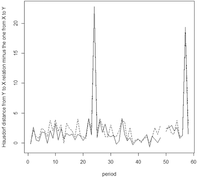

  

  The solid line depcits the Hausdorff average distance for relations from MSP (or Y) to MHP (or X), while the dashed line depcits the Hausdorf minimal distance for relations from MSP (or Y) to MHP (or X).

  Judge from the results we obtain, we shall confidently reach a conclusion that military hard power do bolster the monetary soft power, but not the other way around.

Conclusion and recommendations

In this study, we devise a series of procedures to find the causal relations between military hard power and monetary soft power. These procedures utilise various analytical techniques: k-means, optimal empirical surjective relations, absolute causal relations, inner product, data-based conditional probabilities, Hausdorff measures for distance, etc. The result shows there is a clear causal relation that military hard power backs up monetary soft power. The advantages for our approach are it relies less on statistical approaches and thus more flexible in coupling with other mathematical analytical tools. It also saves one from applying interpolation approaches on data generating or fitting—our approach could tackle samples with dynamical sizes. Another advantage is it is easier to interpret the result, since it relies more on mathematical tools, in particular the usage of distance functions provides much more intuitive interpretation.

There are several limitations in our approaches and improvements to be done in the future study. Firstly, we base our inferences on optimal surjective relations. Indeed one could perform fuzzy inferences, though a concise and definite causality might not exist if one takes other surjective or partially surjective relation into consideration. Secondly, other indicators regarding either military hard power or monetary soft power could be included. Thirdly, one could base on this approach to revisit the lasting issue whether military spending contributes to economic growth or the other way around.

There are some recommendations for further research. In this article, we exploit k-means to decide the centroids and clusters. The number of categories for MHP is chosen to be 5 and the one for MSP is chosen to be 4. One could lift such arbitrary choice, and adopt other artificial techniques to decide the choice of the numbers. Moreover, we adopt monetary units to uniformly quantify the military hard power and monetary soft power. Such adoption could be further extended to involve other data, for example, the number of nuclear warheads, the number of military staff, the number of aircraft carriers, etc. As for the monetary soft power, one could also involve interest rates, GDP, and other economic indicators. One could also consider other non-numeric data or fuzzy data. In addition, our approach focuses on measuring the linearity to witness the causal relation. There is no precise relation, such as regressions, constructed. To remedy such disadvantage, one might combine this approach with other methods to measure the exact degree of causal relation for future prediction or analysis.

References

Beckley M (2010) Economic development and military effectiveness. J Strateg Stud 33(1):43–79
Blanchard JMF, Lu F (2012) Thinking hard about soft power: a review and critique of the literature on china and soft power. Asian Perspect 36(4):565–589
DiGiuseppe M (2015) Guns, butter, and debt: Sovereign creditworthiness and military expenditure. J Peace Res 52(5):680–693
Dunne JP, Smith RP (2020) Military expenditure, investment and growth. Def Peace Econ 31(6):601–614
Gala P (2008) Real exchange rate levels and economic development: Theoretical analysis and econometric evidence. Camb J Econ 32(2):1243–1272
Kang JW, Dagli S (2018) International trade and exchange rates. J Appl Econ 21(1):84–105
Liss J (2007) Making monetary mischief: using currency as a weapon. World Policy J 24(4):29–38
Looney RE, Fredericksen PC (1990) The economic determinants of military expenditure in selected East Asian countries. Contemp Southeast Asia 11(4):265–277
Manamperi N (2016) Does military expenditure hinder economic growth? Evidence from Greece and Turkey. J Policy Model 38(6):1171–1193
Nye JS (1990) Soft Power. Foreign Policy 80:153–171
Nye JS (2021) Soft power: the origins and political progress of a concept. J Int Commun. https://doi.org/10.1080/13216597.2021.2019893
Odehnal J, Neubauer J, Dyčka L, Ambler T (2020) Development of military spending determinants in Baltic countries–empirical analysis. Economies 8(3):68
Pham VA (2019) Impacts of the monetary policy on the exchange rate: case study of Vietnam. J Asia Bus Econ Stud 26(2):220–237
Robertson P, Sin A (2015) Measuring hard power: china’s economic growth and military capacity. Def Peace Econ 28(1):91–111
Santamaría PGT, García AA, González TC (2021) A tale of five stories: Defence spending and economic growth in NATO’s countries. PLoS ONE 16(1):e0245260
Su C, Xu Y, Chang HL, Lobont OR, Liu Z (2020) Dynamic causalities between defense expenditure and economic growth in china: evidence from rolling granger causality test. Def Peace Econ 31(5):565–582
THE WORLD BANK (2021a) Broad money growth (annual %). https://data.worldbank.org/indicator/FM.LBL.BMNY.ZG. Accessed Sept 2021
THE WORLD BANK (2021b) Official exchange rate (LCU per US$, period average). https://data.worldbank.org/indicator/PA.NUS.FCRF. Accessed Sept 2021
THE WORLD BANK (2021c) Military expenditure (% of GDP). https://data.worldbank.org/indicator/MS.MIL.XPND.GD.ZS. Accessed Sept 2021
Wilson EJ (2008) Hard power, soft power, smart power. Ann Am Acad Pol Soc Sci 616(1):110–124
Yellinek R, Mann Y, Lebel U (2020) Chinese soft-power in the Arab world-China’s Confucius Institutes as a central tool of influence. Comp Strategy 39(6):517–534
Author information
Authors and Affiliations
Contributions
The author declares he is the sole author of this paper.
Corresponding author
Ethics declarations
Competing interests
The author declares no competing interests.
Ethical approval
Not applicable as this study did not involve human participants.
Informed consent
Additional information
Publisher’s note Springer Nature remains neutral with regard to jurisdictional claims in published maps and institutional affiliations.
Supplementary information
41599_2022_1048_MOESM1_ESM.tex
Whether Growth of Military Hard Power Back up Growth of Monetary Soft Power via Data-driven Probabilistic Optimal Relations: Supporting Appendix
Rights and permissions
Open Access This article is licensed under a Creative Commons Attribution 4.0 International License, which permits use, sharing, adaptation, distribution and reproduction in any medium or format, as long as you give appropriate credit to the original author(s) and the source, provide a link to the Creative Commons license, and indicate if changes were made. The images or other third party material in this article are included in the article’s Creative Commons license, unless indicated otherwise in a credit line to the material. If material is not included in the article’s Creative Commons license and your intended use is not permitted by statutory regulation or exceeds the permitted use, you will need to obtain permission directly from the copyright holder. To view a copy of this license, visit http://creativecommons.org/licenses/by/4.0/.
About this article
Cite this article
Chen, RM. Does the growth of military hard power back up the growth of monetary soft power via data-driven probabilistic optimal relations?. Humanit Soc Sci Commun 9, 32 (2022). https://doi.org/10.1057/s41599-022-01048-0
Received:
Accepted:
Published:
DOI: https://doi.org/10.1057/s41599-022-01048-0