
Abstract
A noticeable increase in drought frequency and severity has been observed across the globe due to climate change, which attracted scientists in development of drought prediction models for mitigation of impacts. Droughts are usually monitored using drought indices (DIs), most of which are probabilistic and therefore, highly stochastic and non-linear. The current research investigated the capability of different versions of relatively well-explored machine learning (ML) models including random forest (RF), minimum probability machine regression (MPMR), M5 Tree (M5tree), extreme learning machine (ELM) and online sequential-ELM (OSELM) in predicting the most widely used DI known as standardized precipitation index (SPI) at multiple month horizons (i.e., 1, 3, 6 and 12). Models were developed using monthly rainfall data for the period of 1949–2013 at four meteorological stations namely, Barisal, Bogra, Faridpur and Mymensingh, each representing a geographical region of Bangladesh which frequently experiences droughts. The model inputs were decided based on correlation statistics and the prediction capability was evaluated using several statistical metrics including mean square error (MSE), root mean square error (RMSE), mean absolute error (MAE), correlation coefficient (R), Willmott’s Index of agreement (WI), Nash Sutcliffe efficiency (NSE), and Legates and McCabe Index (LM). The results revealed that the proposed models are reliable and robust in predicting droughts in the region. Comparison of the models revealed ELM as the best model in forecasting droughts with minimal RMSE in the range of 0.07–0.85, 0.08–0.76, 0.062–0.80 and 0.042–0.605 for Barisal, Bogra, Faridpur and Mymensingh, respectively for all the SPI scales except one-month SPI for which the RF showed the best performance with minimal RMSE of 0.57, 0.45, 0.59 and 0.42, respectively.
Introduction
Drought is a natural disaster that affects society and the environment frequently1,2. It significantly influences water resources availability, agricultural production, environmental health and thus, socio-economy of a region3,4. There is no definite way of defining drought because it is not possible to determine the exact duration of a drought event. Drought slowly builds over time and leaves a prolonged influence over a large geographical space without any significant infrastructural damage5,6. The complexity of a drought event is characterized by its duration, intensity, and severity. In a simple term, drought is defined as the period of a temporary shortage of water resources due to persistently low precipitation.
Drought can have different forms, such as meteorological drought, hydrological drought, agricultural drought, and socioeconomic drought7,8,9. Meteorological droughts occur due to deficiency of precipitation from the average. It is the initiator of all other kinds of droughts and therefore, most widely studies for monitoring droughts10. Meteorological drought frequency does not depend on the average precipitation of an area, rather the variability of precipitation. The large variability of precipitation on the deficit side indicates droughts. Therefore, it can occur in any climatic regions including tropical region like Bangladesh11,12 or humid climate zone like Malaysia13,14. Even it can happen in northeast India, the highest rainfall region of the world15. A recent study suggests that the wetter parts of the earth would experience more devastating droughts in future16. It urges more attention to be given for monitoring and forecasting droughts in tropical regions. Droughts are often more devastating when it occurs in tropical regions as the ecosystem of such region is habituated with high year-around rainfall17.
Bangladesh, located in tropical South Asia experienced several devastating droughts due to shortfalls in precipitation18. The droughts caused prolonged water shortages and consequently affected agriculture, environment, and health19. Factors that intensify the impact of drought include population growth, agricultural expansions, land use changes, and industrial development due to associated increase in water demand20. There is a need to have a proper understanding and modeling of drought to ensure sustainable planning and management of water resources. However, the slowly emerging characteristics of droughts causes a challenge in determining and modeling of drought duration, intensity, severity, spatial extent and inter-arrival period21,22.
Drought is a common natural disaster in Bangladesh which generally occurs twice in a decade23. Agricultural damages from drought are more frequent in the country compared to any other natural disasters24. Therefore, a large number of studies have been conducted to characterize meteorological droughts in Bangladesh in recent years25,26,27,28. Besides studies have been conducted to assess drought risk18 and impacts on droughts in agriculture24, economy, water resources29 and society30. However, no studies have been conducted so far to forecast droughts in Bangladesh, though it is highly important for the country from a socio-economic point of view, particularly in the context of climate change.
The rainfall of Bangladesh is changing due to the changes in global climate18,31. This has caused a rise in weather extremes32 and hydrological disasters23 in the country. Mohsenipour et al.23 reported an increase in the return period of droughts in highly drought-prone regions of Bangladesh due to rises in temperature and changes in rainfall pattern. More economic damages due to frequent droughts can be anticipated in future due to climate change. The persistent negative impact of drought on water resources and associated water scarcity and economic damages demands the development of models for the effective prediction and monitoring of drought to ensure a proper establishment of strategies for the management of drought-related risks33,34,35. Improper drought prediction always results in poor drought management, hence, there is a need to build fast, reliable and accurate models for drought prediction which can provide quantitative data on impending drought-related risks. With such models, drought episodes can be accurately predicted by anticipating future changes in drought indices based on information derived from current and historical hydro-meteorological data36,37,38.
A large number of DIs has been developed for monitoring droughts10,26. Among all, the standardized precipitation index (SPI) is the most simple, statistically robust, comprehensible, and independent of climatic factors19. Despite the recent introduction of SPI39, it has been widely accepted in the drought prediction community as a useful DI and has been used in numerous studies to investigate drought variability when assessing the impact of drought in agricultural and hydrological sectors11,26,40.
Several forecasting models have been introduced for forecasting droughts such as autoregression integrated moving average (ARIMA), multiple linear regression (MLR) and Markov Chain41. SPI is a probabilistic index derived from a tailed distribution of rainfall deficit. Therefore, the scale of SPI is not linear. This has made the forecasting of droughts using conventional statistical methods more challenging. Most recently, the applications of machine learning (ML) models have exhibited outstanding progress on modeling drought indices and climatology42,43. Several versions of ML models have been developed for SPI forecasting including artificial neural network (ANN), support vector regression (SVR), extreme learning machine (ELM), adaptive neuro-fuzzy inference system (ANFIS), M5 Tree (M5T), random forest (RF), linear genetic programming (LGP), least-square support vector regression (LSSVR), extremely randomized tree (ERT), multivariate adaptive regression spline (MARS), wavelet preprocessing integrated ML models and bio-inspired hybrid ML models38,44,45,46,47,48,49,50,51. Although there have been diverse models introduced for modeling DIs, it is difficult for scientists and scholars to determine a generalized or a perfect model that can suit all types of climates. Besides, there is a chance of misleading in model development if the non-appropriate variables of models’ structure are set-up. Furthermore, every region behaves differently following the weather stochastics and historical characteristics.
The current research is devoted to the development of machine learning models for SPI forecasting for Bangladesh. Five different versions of machine learning models were developed (RF, MPMR, M5tree, ELM and OSELM) for forecasting SPI at multiple time-scales (1, 3, 6 and 12 months). One-month SPI indicates a short-period deficit of rainfall which affect ecology, air temperature and public health of the country52. Three- and six-month SPIs are used to assess agricultural drought in Bangladesh53, while nine- and twelve-month SPIs are responsible for declination of river flow and groundwater level or hydrological droughts. Therefore, models were developed for forecasting SPI of those five time-scales. The models were developed only for four stations (i.e., Barisal, Bogra, Faridpur and Mymensingh), each representing individual climate zone where droughts usually occur in Bangladesh. Among the six major geographical regions of Bangladesh54, droughts mostly occur in the north, central, central-north and southwest regions. Therefore, models were developed for forecasting droughts at Barisal, Bogra, Faridpur and Mymensingh representing southeast, north, central and central-north regions of Bangladesh. Historical data of 64 years (1949–2013) was used to develop and validate the model.
Materials and methods
Case study
Bangladesh is located in the deltas of large rivers flowing from the Himalayas covers an area of 144,000 km2 (Fig. 1, https://www.diva-gis.org/gdata). A tropical humid climate dominates in most of the country. The minimum temperature of the country goes below 12.8 °C in January while the maximum temperature goes above 31.1 °C in May. Due to an extremely flat topography of the country, the spatial variability of temperature is very low. The orientations of temperature gradient are different for different seasons. Therefore, overall there is very less variability in annual mean temperature among different geographical regions. The rainfall in Bangladesh ranges between 1600 and 4400 mm in the northwest and northeast respectively. Seasonal and annual variability of rainfall is very high. About 75% to annual rainfall occurs in monsoon months of May to September and only 3% rainfall occurs during December–February. The coefficient of annual variability of monsoon rainfall in more than 30% in a major portion of the country. The high variability of rainfall often causes droughts in the country. The country experienced major droughts in the years, 1963, 1966, 1968, 1973, 1977, 1979, 1982, 1989, 1992 and 1994–1995.

The locations of the studied meteorological stations in Bangladesh.
Theoretical overview and SPI calculation
The review of ML models used in this study, RF, MPMR, M5tree, ELM and OSELM are provided in this section.
Random Forest (RF)
The RF is created based on the concept of ensemble and bagging learning approach55. It uses the decision tree methodology which performs the bagging procedure for solving the regression problem55,56. Each node in RF is separated randomly by selecting the most important input predictors to enhance the learning process that leads to better prediction accuracy as well as maintaining the robustness to avoid overfitting57. The steps are followed to construct an RF model:
-
i.
Select random k data points from training data.
-
ii.
Construct the decision tree associated with the data in (i).
-
iii.
Choose the n-decision tree (ntrees) that needs to build.
-
iv.
Repeat i and ii.
-
v.
Cumulate the aggregative predictions of ntrees to forecast multi-scaler SPI.
The capacity of the RF has been approved in modeling different phenomena in atmospheric, hydrological and geosciences engineering58, environmental management59, drought forecasting60, rainfall forecasting61, solar index estimation62 and most recently forecasting soil moisture63.
For more comprehensive studies on RF model, readers are referred to57,64,65,66. The flowchart of the random forest model is provided in Fig. 2a.


(a) Schematic view of RF model, (b) Basic structure of ELM model, (c) Representation of M5tree model, (d) The schematic view of MPMR model.
The extreme learning machine (ELM)
ELM designed by Huang et al. is an advanced data intelligent model that uses Single Layer Feed forward Neural Network (SLFN)67. ELM is very fast and more efficient than the existing data-driven models68. Mathematically the ELM can be formulated as69:
where \({\rho }_{i}= {\left[{\rho }_{1}, {\rho }_{2},\ldots ,{\rho }_{M}\right] }^{T}\) is the output weight vector between the hidden layer of M nodes to the m ≥ 1 output nodes, and \({h}_{i}\left({x}_{i}\right)= {\left[{h}_{1}\left(x\right), {h}_{2}\left(x\right),\ldots ,{h}_{M}\left(x\right)\right] }^{T}\) is ELM nonlinear feature mapping and \({f}_{M}\left(x\right)\) is the final ouptput/prediction. For example, the output (row) vector of the hidden layer with respect to the input \(x.\) \({h}_{i}\left(x\right)\) is the output of the ith hidden node output. The output functions of hidden nodes may not be unique. Different output functions may be used in different hidden neurons. In real life problems \({h}_{i}\left({x}_{i}\right)\) can be written as:
where \(G\left(a,b,x\right)\) (with hidden node parameters (a, b)) is a nonlinear piecewise continuous function satisfying ELM universal approximation capability theorems and \(R\) is the set of real numbers whereas \({R}^{d}\) is the d-dimensional set of real numbers and \({x}_{i}\) is the input data. The commonly used mapping function/activation function in ELM are Sigmoid function, Hyperbolic tangent function, Gaussian function, Hard limit function, Cosine function and Fourier basis functions. ELM trains an SLFN in random feature mapping and linear parameters solving phases. First ELM randomly adjusts the hidden layer to map the input predictor into a feature space with the help of some nonlinear functions. The random feature phase differentiates ELM from SVM and deep neural networks. The nonlinear activation functions are basically nonlinear piecewise continuous functions. The hidden node parameters (a, b) in ELM are randomly created which are independent of the training data.
In the second phase of ELM learning, the weights connecting the hidden layer and the output layer, represented by \(\rho\), are solved by reducing the approximation error in the squared error sense:
where \(H\) is the hidden layer output matrix which can be simplified as follows69.
and \(T\) is the training data matrix, which can be written as:
The ∥ · ∥ denotes the Frobenius norm. The optimum solution to (3) is given by:
Here \({\rm H}^{+}\) is the Moore–Penrose generalized inverse of matrix of H. The principle which differentiates ELM from the conventional neural network model is that every parameter of the feed-forward networks (input weights and hidden layer biases) is not necessary to be fine-tuned. The SLFNs with randomly selected input weights effectively learn different training patterns with minimum error. Following randomly selecting input weights and the hidden layer biases, SLFNs can be deemed as a linear system. The output weights which connect the hidden layer to the output layer of this linear system can now be systematically solved by generalized inverse operation of the hidden layer output matrices. This makes ELM model many times faster than that of conventional feedforward learning algorithms. The flowchart of ELM model is shown in Fig. 2b.
The online sequential extreme learning machine (OSELM)
A standalone ELM which uses all N-samples data for the training. However, the data chunk-by-chunk may be used in solving real-world complexity because the process of learning is a very time consuming and requires new data for training ELM each time the model is run70. The OSELM performs in two learning stages as the variant of a standalone ELM model, i.e., a sequential learning stage and initialization stage. In the initialization stage, for a given training dataset \({\aleph }_{k-1}\):
where \({x}_{j}\) is the input data point and \({t}_{j}\) is the jth parameter. The initial output weight is given by:
where \({\rho }_{k-1}\) is the initial output weight, \({\theta }_{k-1}={\left({H}_{k-1}^{t}{H}_{k-1}\right)}^{-1}\) is the Moore–Penrose generalized inverse of matrix, \({{H}_{k-1}=\left[{h}_{1}^{t}, \ldots ,{h}_{k-1}^{t}\right]}^{t}\) is the hidden layer output matrix, and \({{T}_{k-1}=\left[{t}_{1}, \ldots ,{t}_{k-1}\right]}^{t}\) is the training data matrix.
The biases and random weights are assigned to the small chunk in the initialization stage to compute the hidden layer output matrix in the initial SPI (W) training data. The sequential learning phase is then initiated where RLS algorithm is employed to update the output weights in a recursive way70. The output weights in OSELM are recursively updated based on the intermediate results in the last iteration and the newly arrived data, which is discarded instantly once they have been learnt, and therefore, the calculation overhead and the memory requirement of the algorithm are significantly decreased. The readers can consult literature for further details on OS-ELM71,72,73.
The M5 tree (M5tree) model
The M5tree model works on the binary decision tree structure, is an ordered and hierarchical model74. The connection is initiated between inputs and output at the terminal nodes using linear regression75. Tree-based models are made according to a divide-and-conquer method for establishing a relationship between the inputs and output76. Two steps are involved to build the M5tree model i.e. In the first step, the data is partitioned into subsets to create model tree which is based on standard deviation that reaches a node as a measure of error and determining the expected decrease in the error as a result of testing each attribute77. The method is recursive in which the data points are divided into subsets similar to a test that depends on the standard deviation and the error depletion \({\lambda }_{R}\) as given77,78:
where \(\lambda\) is set of examples that reach the nodes and \({\Gamma }_{j}\) is a subset of examples that have the \(jth\) output of the potential set outputs while \({\lambda }_{R}\) is the standard deviation. Due to branching procedure, data in child nodes have fewer \({\lambda }_{R}\) than parent nodes. A structure is selected that has the maximum expected error reduction by analyzing all possible structures. This dividing and conquering rule frequently produces a great tree-like structure that leads to overfit and to prevent overfitting, the overgrown tree is pruned, and pruned subtrees are substituted with linear regression functions in the second step. General form of the model is77:
where \({a}_{0}{, a}_{1}, {a}_{2}\) are the linear regression constants. Figure 2c represents the basic structure of M5tree model.
The minimax probability machine regression (MPMR) model
The MPMR is a probabilistic, nonlinear regressor model which increase the least probability in the correct regression interval of the objective function. The MPMR is using convex optimizations and linear discriminant79, which make MPMR a good and improved version of Support Vector Machine79. The data is calculated among \(+\delta\) and \(-\delta\) with the axis of a dependent variable by shifting all of the regression data. The boundary between the two is a regression surface, where the upper and lower bounds of probability are identified for misclassifying a point without making distributional assumption80. The learning (D-dimensional) inputs are generated from undefined regression as follows:
where a ∈ RD is an input vector according to a bounded distribution \(\Omega\) whereas Y ∈ R is an output vector, and variance \(\rho ={\sigma }^{2}\in R\). MPMR sets an approximation function \(\hat{f}\), where for \({x}_{i}\) generated from \(\Omega\):
The bounds are determined by model based on minimum probability (\(\omega\)), that \(\hat{f}(a)\) is within \(\varepsilon\) of Y79:
By minimax probability presented in Eq. (13), the prediction power of a true regression is calculated by a bound-on minimax probability. Hence, deducing \(\omega\) within \(\varepsilon\) of the true function80. The MPMR model is built based on kernel function,
where \({K}_{i,j}=\Delta \left({a}_{i},{a}_{j}\right)\) is the kernel function based on Mercer condition, \({a}_{i}\) is from the learning data, \({\chi }_{i}\) and \(\varphi\) are the output parameters. The schematic view of MPMR model is shown in Fig. 2d.
Multi-scale standardized precipitation index (SPI)
The SPI quantifies the wet and dry scenarios based on statistical probability theory. Before developing the forecasting models, the multi-scale SPI index was calculated from rainfall (RnF) time-series39 using a gamma distribution function (\(g(RnF)\)):
where α and β are the parameters determined by maximum likelihood estimator, and \(\Gamma (\alpha )\) is the mathematical gamma function. The cumulative probability (\(G(RnF)\)) is defined as:
By substituting t = RnF/β, Eq. (16), \(G(RnF)\) becomes:
The cumulative probability reduces to the following form when RnF = 0:
with p represents the probability of zero which determines the SPI index as:
where \({\varepsilon }_{0},{\varepsilon }_{1},{\varepsilon }_{2},{\varepsilon }_{3}\), \({\omega }_{1},{\omega }_{2}\) and \({\omega }_{3}\) are arbitrary constants with magnitudes: \({\varepsilon }_{0}=2.515517\), \({\varepsilon }_{1}=0.802853\), \({\varepsilon }_{3}=0.010328\), \({\omega }_{1}=1.432788\), \({\omega }_{2}=0.189269\) and \({\omega }_{3}=0.001308\)39. Drought is categorized into three as moderate = (− 1.5 < SPI ≤ 1.0), severe = (− 2.0 < SPI ≤ − 1.5), and extreme = (SPI ≤ − 2.0). The time series of the generated SPI for different scales at all the four meteorological stations are presented in Fig. 3.

The time series of the generated SPI for the four meteorological stations.
Models development and evaluation metrics
The forecasting models were developed in MATLAB R2016b programming environment (The Math Works Inc. USA). By operating Pentium 4, 2.93 GHz dual-core Central Processing Unit, all the simulations were obtained. Historical rainfall data was used to compute the SPI for 64 years. The training phase was built using 75% of the data (1949–1997) while the testing was conducted with the remaining 25% data (1998–2013). These forecasting ML models were developed using the steps as follow:
- Step 1::
-
Computing Partial autocorrelation functions (PACFs) of SPI1, SPI3, SPI6 and SPI12 to estimate the significant lags. The PACF was estimated for SPI1, SPI3, SPI6 and SPI12 using following equation81:
$${\sigma }_{l}=\frac{\frac{1}{n-l}{\sum }_{t=l+1}^{n}\left(SP{I}_{t}-\overline{SPI}\right)\left(SP{I}_{t-l}-\overline{SPI}\right)}{\sqrt{\frac{1}{n}{\sum }_{t=1}^{n}\left(SP{I}_{t}-\overline{SPI}\right)}\sqrt{\frac{1}{n-l}{\sum }_{t=l+1}^{n}\left(SP{I}_{t-l}-\overline{SPI}\right)}}$$(20)where \(SP{I}_{t}\) is the observed series; \(l = 0,1,2, \ldots\) for \(t = 1,2,3, \ldots ,n\); and \(\overline{SPI}\) denotes mean SPI. The PACF is defined as:
$$SP{I}_{t}={\Gamma }_{21}SP{I}_{t-1}+{\Gamma }_{22}SP{I}_{t-1}+{E}_{t}$$(21)where \({\Gamma }_{22}\) indicates that the order 2 PACF is expected to yield. A greater positive value of PACF indicates a good input for drought forecasting model development. Figure 4a–d present the statistical correlations estimated for the investigated stations.
Figure 4 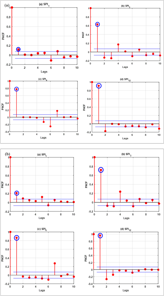
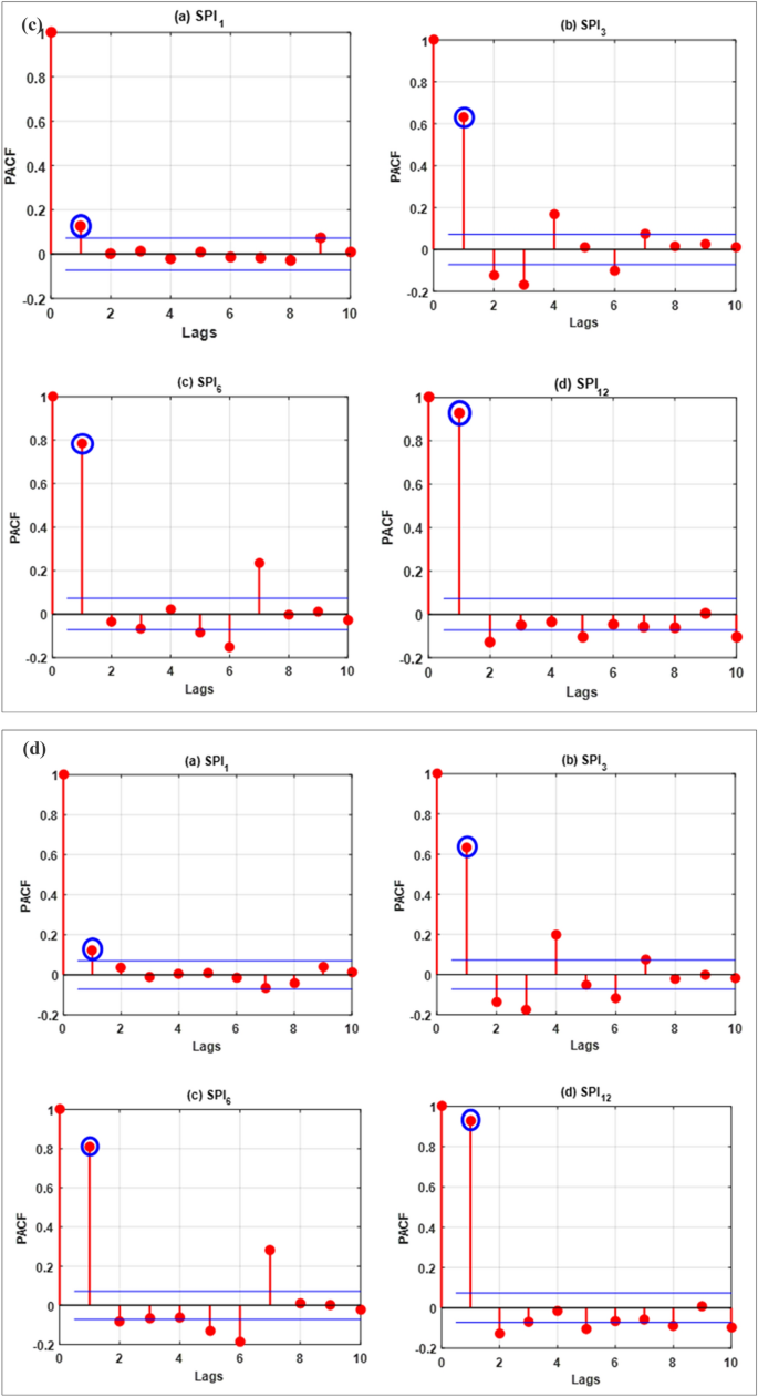
The correlation statistics of the lags for all the inspected meteorological time series data (a) Barisal station, (b) Bogra station, (c) Faridpur station and (d) Mymensingh station.
- Step 2::
-
Normalization process
The normalization process is essential for data scaling to solve the problem of high variation in data. In this study, data were scaled between [0, 1] using Eq. (17):
$$SP{I}_{norm}=\frac{\left(SPI-SP{I}_{min}\right)}{\left(SP{I}_{max}-SP{I}_{min}\right)}$$(22)In Eq. (17), \(SPI\) represents the input/output, \(SP{I}_{min}\) is the minimum SPI value, \(SP{I}_{max}\) is the maximum SPI value and \(SP{I}_{norm}\) is the value corresponding normalized numeric.
- Step 3::
-
Applying data intelligent methods.
The data were divided into 70–30% for the training and testing the models. The number of trees (1000) was defined before developing the RF model. Different activation functions (hardlim, radial basis, sine, sigmoid) were evaluated to determine the best activation function for various numbers of unseen neurons in the range from 1 to 50 before development of OSELM and ELM models. The size of the block was set to 100 for OSELM. The significant lags at (t-1) were used in M5tree and MPMR models to forecast SPI1, SPI3, SPI6 and SPI12. For the development of MPMR model, the linear, polynomial and Gaussian kernels were used.


Several performance metrics were computed for the evaluation of model performance including mean square error (MSE), correlation coefficient (R), Willmott’s Index of agreement (WI), Nash Sutcliffe efficiency (NSE), root mean square (RMSE), mean absolute error (MAE) and Legates and McCabe Index (LM)82,83,84,85. The mathematical expression of the metrics are as follows:
where \({SPI}_{o}\) and \({SPI}_{f}\) are observed and predicted SPI values. \({\overline {SPI}}_{o}\) and \({\overline {SPI}}_{f}\) are the mean of the observed and predicted SPI values. n is the number of sample in the dataset. RMSE provides more weight to higher different between observed and modelled SPIs in estimating model error and therefore, it provides a better estimation of model performance and most widely used by modellers to derive the conclusion.
Results and discussion
Drought prediction for Bangladesh was conducted in this study using the SPIs for different time-scales (1, 3, 6, 9 and 12 months) at four meteorological stations distributed over the country (e.g. Barisal, Bogra, Faridpur and Mymensingh). The prediction process was conducted using relatively new ML models such as RF, MPMR, M5tree, ELM and OSELM. To build the predictive models, the correlated antecedent SPI values were used as inputs.
The employed predictive models were trained using 50-year monthly data (1949–1997) while the testing was conducted using 16-year data (1998–2013) at all the four stations. To enhance the accuracy in prediction of SPI, all predictive variables were standardized in a range of 0 to 1. Adequacy of each predictive model was quantified using performance indices such as MSE, R, WI, NSE, RMSE, MAE and LM (Eqs. (18–24)). The predictive models were compared based on their performance during the testing phase.
The performance of the models in terms of statistical metrics is shown in Tables 1, 2, 3, 4. The results revealed that RF is the best predictive model for SPI-1 (\(RMSE=0.43{-}0.54\)) at all stations while for the other scales of SPI such as SPI-3 (\(RMSE=0.2{-}0.72\)), SPI-6 (\(RMSE=0.09{-}0.22\)) and SPI-12 (\(RMSE=0.03{-}0.08\)) both ELM and OSELM showed superiority compared to others. However, the obtained results using ELM (\(RMSE=0.37\)) showed a bit higher accuracy compared to OSELM (\(RMSE=0.72\)) at Faridpur station for SPI-3. The M5tree (\(RMSE=0.4{-}0.94\)) and MPMR (\(RMSE=0.37{-}0.84\)) showed the lowest performance in predicting SPI for all the scales. Hence, it can be concluded that ELM is the best performing model while M5tree has the lowest accuracy in prediction of SPI. All predictive models showed better accuracy in predicting SPI for higher scales. This evidenced the potential of non-tuned extreme learning machine model in forecasting droughts in Bangladesh. Recently, the feasibility of the ELM model is successfully implemented for drought indices simulation in many other studies44,86,87.
The graphical evaluation and assessment among the predictive models in term of standardized performance indices are depicted in a form of Heatmap diagram in Fig. 5. The dark blue color in the figure represents the best statistical performance while dark red color represents the worst performance. It can be seen from the figure that ELM and OSELM showed the best performance in term of all metrics for all SPIs except SPI-1. Furthermore, ELM showed the highest performance compared to other models at all stations. Besides, the maximum number of dark red cells (worst predictive model) was shown by M5tree model.


Heat map showing the performance of different predictive models in terms of different statistics metrics at the four investigated meteorological stations and multiple SPI scales.
Taylor diagram is another graphical presentation which was used to make a comparison among the employed predictive models (Fig. 6). The results of Taylor diagrams indicated good consistency with the obtained performance indices. Figure 6 shows that the highest agreement exists between the RF prediction (blue rectangular) and observed SPI-1 at all the stations. For other SPI scales, ELM and OSELM showed relatively same results which indicate their superiority compared to other predictive models. These models provided the lowest normalized RMSE (less than 0.4), the highest correlations (more than 0.95) and the lowest variation (within 0.6–0.9). However, ELM provided better results for SPI-3 in Faridpur station compared to OSELM while at other stations and SPI scales the results were found the same.


Taylor diagram presentation of the performance of the predictive models at four investigated meteorological stations and multiple SPI scales.
Scatter plots shows the linear correlation between observed and predicted SPI values at all stations (Fig. 7). The results revealed that the prediction of all the predictive models except M5tree and MPMR have a high correlation with observation. Most of the predicted points are aligned to the perfect line (45° line) which shows a significant performance of prediction models. Based on the obtained values of correlation coefficients, it can be seen that OSELM (\(R=0.81{-}0.96\)) has better correlation for SPI-1 at all stations except Faridpur (\(R=0.74\)). However, it can be concluded that the best correlation for SPI-1 was attained using OSELM and the worst results by M5tree (\(R=-0.006{-}0.011\)). For other SPI scales, it is clear that ELM provided a higher accuracy compared to other models. However, there was no significant difference between the results obtained using ELM (\(R=0.98{-}0.999\)) and OSELM (\(R=0.69{-}0.999\)) at all the considered stations. Therefore, both the ELM and OSELM models indicated a higher correlation between the observed and predicted SPI for different scales in comparison with RF, MPMR and M5tree models. The M5tree (\(R=-0.006{-}0.011\)) provided the lowest correlation coefficient. Overall, it can be remarked that both ELM and OSELM models have adequate capability in SPI prediction.


The scatter plot between the observed and predicted SPI obtained using the predictive models at the four investigated meteorological stations and multiple SPI scales.
To assess the uncertainty in SPI prediction, 25%, 50% and 75% quantile values of the observed and predicted SPI are presented using boxplots in Fig. 8. The figure shows that the variability in SPI-1 values could not be simulated by any of the models adequately. Many predicted SPI-1 values were found fluctuating near to zero (narrow range) while the observed values have a wide range [− 2 to 2]. However, the RF model showed better accuracy to simulate variability and quartiles of SPI-1 compared to others. All predictive models were found to show better results in simulating SPI quantiles of other SPI scales, especially for their higher orders. Overall, the ELM and OSELM provided the highest accuracy to simulate the variability of SPI values while M5tree showed the worst. Hence, it can be remarked that M5tree is not suitable for prediction of SPI in any regions of Bangladesh.


Box plot presentation of the performance of the predictive models at the four investigated meteorological stations and multiple SPI scales.
Conclusions
The current research is attempted to investigate the feasibility of newly developed ML models to forecast multiple scales of SPI drought index over Bangladesh. The developed predictive models are inspected on the monthly scale of rainfall data for the period of 1949–2013 at four different meteorological stations. The predictors of the forecasting models were accomplished using the potential of the statistical auto-correlation method. The attained forecasting results demonstrate consistency in results obtained using ELM for the 3-, 6- and 12-month SPI. It showed the minimal RMSE (0.33, 0.15 and 0.06), (0.35, 0.21 and 0.08), (0.36, 0.20 and 0.05) and (0.020, 0.09 and 0.02) at Barisal, Bogra, Faridpur and Mymensingh meteorological stations in predicting the SPI-3, SPI-6 and SPI-12, respectively. Whereas, the RF showed the best performance for one-month SPI with minimal RMSE values of 0.57, 0.45, 0.59 and 0.42 for those four stations. The results indicate the potential of the models to be employed for drought forecasting in Bangladesh for the mitigation of drought impacts. In future, other ML models can be employed to evaluate their performance in forecasting droughts in Bangladesh. Besides, different optimization methods can be used for the optimization of ML model parameters to improve their prediction capability.
Data availability
The used dataset in this research are available upon request from the corresponding author.
References
Mishra, A. K. & Singh, V. P. A review of drought concepts. J. Hydrol. 391, 202–216 (2010).
Mishra, A. K. & Singh, V. P. Drought modelling—A review. J. Hydrol. 403, 157–175 (2011).
Samarah, N. H. Effects of drought stress on growth and yield of barley. Agron. Sustain. Dev. https://doi.org/10.1051/agro (2005).
Dai, A. Drought under global warming: A review. Wiley Interdiscip. Rev. Clim. Change https://doi.org/10.1002/wcc.81 (2011).
Reddy, A. R., Chaitanya, K. V. & Vivekanandan, M. Drought-induced responses of photosynthesis and antioxidant metabolism in higher plants. J. Plant Physiol. https://doi.org/10.1016/j.jplph.2004.01.013 (2004).
Passioura, J. B. Drought and drought tolerance. Plant Growth Regul. https://doi.org/10.1007/BF00024003 (1996).
Wilhite, D. A. & Glantz, M. H. Understanding: The drought phenomenon: the role of definitions. Water Int. 10, 111–120 (1985).
Qutbudin, I. et al. Seasonal drought pattern changes due to climate variability: Case study in Afghanistan. Water 11, 1096 (2019).
Nguyen-Huy, T., Deo, R. C., Yaseen, Z. M., Prasad, R. & Mushtaq, S. Bayesian Markov chain Monte Carlo-based copulas: factoring the role of large-scale climate indices in monthly flood prediction. In Intelligent Data Analytics for Decision-Support Systems in Hazard Mitigation 29–47 (Springer, Berlin, 2020).
Ahmed, K., Shahid, S., Chung, E.-S., Wang, X. & Harun, S. B. Climate change uncertainties in seasonal drought severity-area-frequency curves: Case of arid region of Pakistan. J. Hydrol. 570, 473–485 (2019).
Shahid, S. Spatial and temporal characteristics of droughts in the western part of Bangladesh. Hydrol. Process. https://doi.org/10.1002/hyp.6820 (2008).
Alamgir, M. et al. Evaluating severity–area–frequency (SAF) of seasonal droughts in Bangladesh under climate change scenarios. Stoch. Environ. Res. Risk Assess. https://doi.org/10.1007/s00477-020-01768-2 (2020).
Fung, K. F., Huang, Y. F. & Koo, C. H. Assessing drought conditions through temporal pattern, spatial characteristic and operational accuracy indicated by SPI and SPEI: Case analysis for Peninsular Malaysia. Nat. Hazards 103, 2071–2101 (2020).
Tan, M. L., Juneng, L., Tangang, F. T., Chan, N. W. & Ngai, S. T. Future hydro-meteorological drought of the Johor River Basin, Malaysia, based on CORDEX-SEA projections. Hydrol. Sci. J. https://doi.org/10.1080/02626667.2019.1612901 (2019).
Ray, D. K., Gerber, J. S., Macdonald, G. K. & West, P. C. Climate variation explains a third of global crop yield variability. Nat. Commun. https://doi.org/10.1038/ncomms6989 (2015).
Ukkola, A. M., De Kauwe, M. G., Roderick, M. L., Abramowitz, G. & Pitman, A. J. Robust future changes in meteorological drought in CMIP6 projections despite uncertainty in precipitation. Geophys. Res. Lett. https://doi.org/10.1029/2020GL087820 (2020).
Laura Suarez, M. & Kitzberger, T. Differential effects of climate variability on forest dynamics along a precipitation gradient in northern Patagonia. J. Ecol. 98, 1023–1034 (2010).
Shahid, S. & Behrawan, H. Drought risk assessment in the western part of Bangladesh. Nat. Hazards https://doi.org/10.1007/s11069-007-9191-5 (2008).
Keyantash, J. & Dracup, J. A. The quantification of drought: An evaluation of drought indices. Bull. Am. Meteorol. Soc. 83, 1167–1180 (2002).
Barros, V. et al. IPCC, 2012—Glossary of Terms. Managing the Risks of Extreme Events and Disasters to Advance Climate Change Adaptation (2012) https://doi.org/10.1177/1403494813515131
Deo, R. C., Kisi, O. & Singh, V. P. Drought forecasting in eastern Australia using multivariate adaptive regression spline, least square support vector machine and M5Tree model. Atmos. Res. https://doi.org/10.1016/j.atmosres.2016.10.004 (2017).
Sohn, S. J., Tam, C. Y. & Ahn, J. B. Development of a multimodel-based seasonal prediction system for extreme droughts and floods: A case study for South Korea. Int. J. Climatol. 33, 793–805 (2013).
Mohsenipour, M., Shahid, S., Chung, E. S. & Wang, X. J. Changing pattern of droughts during cropping seasons of Bangladesh. Water Resour. Manag. https://doi.org/10.1007/s11269-017-1890-4 (2018).
Mundial, B. Water resource management in Bangladesh: Steps towards a new national water plan. In Water resource management in Bangladesh: Steps Towards a new national water plan (Banco Mundial, 1998).
Dash, B. K., Rafiuddin, M., Khanam, F. & Islam, M. N. Characteristics of meteorological drought in Bangladesh. Nat. Hazards 64, 1461–1474 (2012).
Alamgir, M. et al. Analysis of meteorological drought pattern during different climatic and cropping seasons in Bangladesh. J. Am. Water Resour. Assoc. 51, 794–806 (2015).
Amin, A. et al. Evaluation and analysis of temperature for historical (1996–2015) and projected (2030–2060) climates in Pakistan using SimCLIM climate model: Ensemble application. Atmos. Res. 213, 422–436 (2018).
Mortuza, M. R., Moges, E., Demissie, Y. & Li, H.-Y. Historical and future drought in Bangladesh using copula-based bivariate regional frequency analysis. Theor. Appl. Climatol. 135, 855–871 (2018).
Rahman, A. T. M. S., Jahan, C. S., Mazumder, Q. H., Kamruzzaman, M. & Hosono, T. Drought analysis and its implication in sustainable water resource management in Barind area, Bangladesh. J. Geol. Soc. India 89, 47–56 (2017).
Habiba, U., Shaw, R. & Takeuchi, Y. Drought risk reduction through a socio-economic, institutional and physical approach in the northwestern region of Bangladesh. Environ. Hazards 10, 121–138 (2011).
Rimi, R. H., Haustein, K., Allen, M. R. & Barbour, E. J. Risks of pre-monsoon extreme rainfall events of Bangladesh: Is anthropogenic climate change playing a role?. Bull. Am. Meteorol. Soc. 100, S61–S65 (2019).
Basher, M. A., Stiller-Reeve, M. A., Saiful Islam, A. K. M. & Bremer, S. Assessing climatic trends of extreme rainfall indices over northeast Bangladesh. Theor. Appl. Climatol. 134, 441–452 (2017).
Wilhite, D. A., Svoboda, M. D. & Hayes, M. J. Understanding the complex impacts of drought: A key to enhancing drought mitigation and preparedness. Water Resour. Manag. https://doi.org/10.1007/s11269-006-9076-5 (2007).
Wang, Q. et al. Assessment of spatial agglomeration of agricultural drought disaster in China from 1978 to 2016. Sci. Rep. https://doi.org/10.1038/s41598-019-51042-x (2019).
Nabaei, S., Sharafati, A., Yaseen, Z. M. & Shahid, S. Copula based assessment of meteorological drought characteristics: Regional investigation of Iran. Agric. For. Meteorol. 276, 107611 (2019).
Zin, W. Z. W., Jemain, A. A. & Ibrahim, K. Analysis of drought condition and risk in Peninsular Malaysia using Standardised Precipitation Index. Theor. Appl. Climatol. 111, 559–568 (2013).
Buttafuoco, G., Caloiero, T. & Coscarelli, R. Analyses of drought events in Calabria (Southern Italy) using standardized precipitation index. Water Resour. Manag. 29, 557–573 (2015).
Rhee, J. & Im, J. Meteorological drought forecasting for ungauged areas based on machine learning: Using long-range climate forecast and remote sensing data. Agric. For. Meteorol. 237–238, 105–122 (2017).
Mckee, T. B., Doesken, N. J. & Kleist, J. The relationship of drought frequency and duration to time scales. In AMS 8th Conference on Applied Climatology 179–184 (1993).
Yaseen, Z. M. & Shahid, S. Drought index prediction using data intelligent analytic models: a review. In Intelligent Data Analytics for Decision-Support Systems in Hazard Mitigation 1–27 (Springer, Berlin, 2020).
Fung, K. F., Huang, Y. F., Koo, C. H. & Soh, Y. W. Drought forecasting: A review of modelling approaches 2007–2017. J. Water Clim. Change https://doi.org/10.2166/wcc.2019.236 (2019).
Malik, A. et al. Drought index prediction using advanced fuzzy logic model: Regional case study over Kumaon in India. PLoS ONE https://doi.org/10.1371/journal.pone.0233280 (2020).
Kisi, O., Choubin, B., Deo, R. C. & Yaseen, Z. M. Incorporating synoptic-scale climate signals for streamflow modelling over the Mediterranean region using machine learning models. Hydrol. Sci. J. 64, 1240–1252 (2019).
Mouatadid, S., Raj, N., Deo, R. C. & Adamowski, J. F. Input selection and data-driven model performance optimization to predict the Standardized Precipitation and Evaporation Index in a drought-prone region. Atmos. Res. 212, 130–149 (2018).
Park, S., Im, J., Jang, E. & Rhee, J. Drought assessment and monitoring through blending of multi-sensor indices using machine learning approaches for different climate regions. Agric. For. Meteorol. 216, 157–169 (2016).
Belayneh, A., Adamowski, J., Khalil, B. & Quilty, J. Coupling machine learning methods with wavelet transforms and the bootstrap and boosting ensemble approaches for drought prediction. Atmos. Res. 172–173, 37–47 (2016).
Deo, R. C. & Şahin, M. Application of the artificial neural network model for prediction of monthly standardized precipitation and evapotranspiration index using hydrometeorological parameters and climate indices in eastern Australia. Atmos. Res. 161–162, 65–81 (2015).
Ali, M., Deo, R. C., Downs, N. J. & Maraseni, T. An ensemble-ANFIS based uncertainty assessment model for forecasting multi-scalar standardized precipitation index. Atmos. Res. 207, 155–180 (2018).
Danandeh Mehr, A., Kahya, E. & Özger, M. A gene-wavelet model for long lead time drought forecasting. J. Hydrol. 517, 691–699 (2014).
Anshuka, A., van Ogtrop, F. F. & Vervoort, R. W. Drought forecasting through statistical models using standardised precipitation index: A systematic review and meta-regression analysis. Nat. Hazards 97, 955–977 (2019).
Zhang, R., Chen, Z.-Y., Xu, L.-J. & Ou, C.-Q. Meteorological drought forecasting based on a statistical model with machine learning techniques in Shaanxi province, China. Sci. Total Environ. 665, 338–346 (2019).
Shahid, S. Recent trends in the climate of Bangladesh. Clim. Res. https://doi.org/10.3354/cr00889 (2010).
Alamgir, M. et al. Parametric assessment of seasonal drought risk to crop production in Bangladesh. Sustainability 11, 1442 (2019).
Pour, S. H., Shahid, S., Chung, E.-S. & Wang, X.-J. Model output statistics downscaling using support vector machine for the projection of spatial and temporal changes in rainfall of Bangladesh. Atmos. Res. 213, 149–162 (2018).
Breiman, L. Bagging predictors. Mach. Learn. 24, 123–140 (1996).
Khosravi, K. et al. Meteorological data mining and hybrid data-intelligence models for reference evaporation simulation: A case study in Iraq. Comput. Electron. Agric. 167, 105041 (2019).
Breiman, L. Random forests. Mach. Learn. 45, 5–32 (2001).
Moore, I. D. D., Grayson, R. B. B. & Ladson, A. R. R. Digital terrain modelling: A review of hydrological, geomorphological and biological applications. Hydrol. Process. 5, 3–30 (1991).
Ascough, J. C., Maier, H. R., Ravalico, J. K. & Strudley, M. W. Future research challenges for incorporation of uncertainty in environmental and ecological decision-making. Ecol. Model. 219, 383–399 (2008).
Chen, J., Li, M. & Wang, W. Statistical uncertainty estimation using random forests and its application to drought forecast. Math. Probl. Eng. 2012, 1–13 (2012).
Ali, M., Deo, R. C., Downs, N. J. & Maraseni, T. Multi-stage hybridized online sequential extreme learning machine integrated with Markov Chain Monte Carlo copula-Bat algorithm for rainfall forecasting. Atmos. Res. 213, 450–464 (2018).
Deo, R. C., Downs, N. J., Adamowski, J. F. & Parisi, A. V. Adaptive neuro-fuzzy inference system integrated with solar zenith angle for forecasting sub-tropical photosynthetically active radiation. Food Energy Security https://doi.org/10.1002/fes3.151 (2018).
Prasad, R., Deo, R. C., Li, Y. & Maraseni, T. Ensemble committee-based data intelligent approach for generating soil moisture forecasts with multivariate hydro-meteorological predictors. Soil Tillage Res. https://doi.org/10.1016/j.still.2018.03.021 (2018).
Liaw, A. & Wiener, M. Classification and regression by randomForest. News 2, 18–22 (2002).
Prasad, R., Deo, R. C., Li, Y. & Maraseni, T. Ensemble committee-based data intelligent approach for generating soil moisture forecasts with multivariate hydro-meteorological predictors. Soil Tillage Res. 181, 63–81 (2018).
Segal, M. R. Machine learning benchmarks and random forest regression. Technical Report (Center for Bioinformatics & Molecular Biostatistics, University of California, San Francisco, CA, 2003).
Huang, G.-B., Zhu, Q.-Y. & Siew, C.-K. Extreme learning machine: Theory and applications. Neurocomputing 70, 489–501 (2006).
Yaseen, Z. M., Sulaiman, S. O., Deo, R. C. & Chau, K.-W. An enhanced extreme learning machine model for river flow forecasting: State-of-the-art, practical applications in water resource engineering area and future research direction. J. Hydrol. 569, 387–408 (2018).
Huang, G., Huang, G. B., Song, S. & You, K. Trends in extreme learning machines: A review. Neural Netw. 61, 32–48 (2015).
Hou, M. et al. Global solar radiation prediction using hybrid online sequential extreme learning machine model. Energies 11, 3415 (2018).
Lan, Y., Soh, Y. C. & Huang, G.-B. Ensemble of online sequential extreme learning machine. Neurocomputing 72, 3391–3395 (2009).
Liang, N.-Y., Huang, G.-B., Saratchandran, P. & Sundararajan, N. A fast and accurate online sequential learning algorithm for feedforward networks. IEEE Trans. Neural Netw. 17, 1411–1423 (2006).
Yadav, B., Ch, S., Mathur, S. & Adamowski, J. Discharge forecasting using an online sequential extreme learning machine (OS-ELM) model: A case study in Neckar River, German. Meas. J. Int. Meas. Confed. 92, 433–445 (2016).
Quinlan, J. R. Learning with continuous classes. Mach. Learn. 92, 343–348 (1992).
Mitchell, T. M. Machine learning and data mining. Commun. ACM. 42, 30–36 (1997).
Rahimikhoob, A., Asadi, M. & Mashal, M. A comparison between conventional and M5 model tree methods for converting pan evaporation to reference evapotranspiration for semi-arid region. Water Resour. Manag. 27, 4815–4826 (2013).
Bhattacharya, B. & Solomatine, D. P. Neural networks and M5 model trees in modelling water level–discharge relationship. Neurocomputing 63, 381–396 (2005).
Sanikhani, H., Deo, R. C., Yaseen, Z. M., Eray, O. & Kisi, O. Non-tuned data intelligent model for soil temperature estimation: A new approach. Geoderma 330, 52–64 (2018).
Strohmann, T. & Grudic, G. Z. A formulation for minimax probability machine regression. In Advances in Neural Information Processing Systems 785–792 (2003).
Bertsimas, D. & Sethuraman, J. Moment problems and semidefinite optimization. Int. Ser. Oper. Res. Manag. Sci. https://doi.org/10.1007/978-1-4615-4381-7_16 (2000).
Hamilton, J. D. Time Series Analysis. Book Vol. 39, xiv (1994).
Chai, T. & Draxler, R. R. Root mean square error (RMSE) or mean absolute error (MAE)? Arguments against avoiding RMSE in the literature. Geosci. Model Dev. 7, 1247–1250 (2014).
Legates, D. R. & Mccabe, G. J. A refined index of model performance: A rejoinder. Int. J. Climatol. 33, 1053–1056 (2013).
Nash, J. E. & Sutcliffe, J. V. River flow forecasting through conceptual models part I—a discussion of principles. J. Hydrol. 10, 282–290 (1970).
Yaseen, Z. M. et al. Novel hybrid data-intelligence model for forecasting monthly rainfall with uncertainty analysis. Water https://doi.org/10.3390/w11030502 (2019).
Deo, R. C. & Şahin, M. Application of the extreme learning machine algorithm for the prediction of monthly Effective Drought Index in eastern Australia. Atmos. Res. 153, 512–525 (2015).
Deo, R. C., Tiwari, M. K., Adamowski, J. F. & Quilty, J. M. Forecasting effective drought index using a wavelet extreme learning machine (W-ELM) model. Stoch. Environ. Res. Risk Assess. https://doi.org/10.1007/s00477-016-1265-z (2016).
Acknowledgements
The authors acknowledge the Bangladesh Meteorological Department (BMD) for providing rainfall dataset.
Author information
Authors and Affiliations
Contributions
Z.M.Y. and S.S. contributed on the conceptualization of the manuscript. S.S. provide the related climate data. M.A. performed the methodology. A.S. conducted the results and discussion. N.A. performed the results investigation and visualization. All authors contributed on the manuscript witting up and editing.
Corresponding author
Ethics declarations
Competing interests
The authors declare no competing interests.
Additional information
Publisher's note
Springer Nature remains neutral with regard to jurisdictional claims in published maps and institutional affiliations.
Rights and permissions
Open Access This article is licensed under a Creative Commons Attribution 4.0 International License, which permits use, sharing, adaptation, distribution and reproduction in any medium or format, as long as you give appropriate credit to the original author(s) and the source, provide a link to the Creative Commons licence, and indicate if changes were made. The images or other third party material in this article are included in the article's Creative Commons licence, unless indicated otherwise in a credit line to the material. If material is not included in the article's Creative Commons licence and your intended use is not permitted by statutory regulation or exceeds the permitted use, you will need to obtain permission directly from the copyright holder. To view a copy of this licence, visit http://creativecommons.org/licenses/by/4.0/.
About this article

Cite this article
Yaseen, Z.M., Ali, M., Sharafati, A. et al. Forecasting standardized precipitation index using data intelligence models: regional investigation of Bangladesh. Sci Rep 11, 3435 (2021). https://doi.org/10.1038/s41598-021-82977-9
Received:
Accepted:
Published:
DOI: https://doi.org/10.1038/s41598-021-82977-9
This article is cited by
-
Identification of influential weather parameters and seasonal drought prediction in Bangladesh using machine learning algorithm
Scientific Reports (2024)
-
Machine learning algorithms for merging satellite-based precipitation products and their application on meteorological drought monitoring over Kenya
Climate Dynamics (2024)
-
Comparative Assessment of Improved SVM Method under Different Kernel Functions for Predicting Multi-scale Drought Index
Water Resources Management (2023)
-
Drought indicator analysis and forecasting using data driven models: case study in Jaisalmer, India
Stochastic Environmental Research and Risk Assessment (2023)
-
Prediction of meteorological drought and standardized precipitation index based on the random forest (RF), random tree (RT), and Gaussian process regression (GPR) models
Environmental Science and Pollution Research (2023)
Comments
By submitting a comment you agree to abide by our Terms and Community Guidelines. If you find something abusive or that does not comply with our terms or guidelines please flag it as inappropriate.
