
Abstract
A computational technique for predicting the DTIs has now turned out to be an indispensable job during the process of drug finding. It tapers the exploration room for interactions by propounding possible interaction contenders for authentication through experiments of wet-lab which are known for their expensiveness and time consumption. Chemogenomics, an emerging research area focused on the systematic examination of the biological impact of a broad series of minute molecular-weighting ligands on a broad raiment of macromolecular target spots. Additionally, with the advancement in time, the complexity of the algorithms is increasing which may result in the entry of big data technologies like Spark in this field soon. In the presented work, we intend to offer an inclusive idea and realistic evaluation of the computational Drug Target Interaction projection approaches, to perform as a guide and reference for researchers who are carrying out work in a similar direction. Precisely, we first explain the data utilized in computational Drug Target Interaction prediction attempts like this. We then sort and explain the best and most modern techniques for the prediction of DTIs. Then, a realistic assessment is executed to show the projection performance of several illustrative approaches in various situations. Ultimately, we underline possible opportunities for additional improvement of Drug Target Interaction projection enactment and also linked study objectives.
Introduction
The accurate prediction of interactions formed between a drug and its targeted protein via computational approaches is highly demanding because it is an efficient analog to the wet-lab experiments that cost heavily and requires additional efforts. Drug–target interactions (DTIs) which are newly discovered are critical for discovering novel targets that can interact with the existing drugs, as well as new drugs that can target some specific genes causing diseases1,2,3. Drug repositioning is one of the efficient methods for the recovery of existing drugs for a novel cause, i.e. drugs which are developed for some particular purposes can be used to treat other biological conditions, meaning a single drug can be applied to many targets4,5. There is already massive research going on the existing drugs based on the bioavailability and their safe use. Repositioning can limit drug costs and may enhance the process of drug discovery, making drug repositioning an eminent method for drug discovery6. Some major techniques employed for the drug repurposing involve network-based approach7, network-based cluster approach8, network-based propagation approach9, text mining-based approach10, and semantics-based approach11. Drug repositioning is different from the traditional drug development that involves five stages, however, this method requires only 4 stages which include compound recognition, obtaining a compound, production and FDA based safety monitoring. The Gleevec (imatinib mesylate) is a well-known example of drug repositioning which was initially thought to interact only with the Bcr-Abl fusion gene related to leukemia. But later on, it was found that interaction of the Gleevec with PDGF and KIT can also be achieved, with an added advantage as a repositioned drug for the treatment of gastrointestinal stromal tumours12,13. The success of Gleevec as a repositioned drug is one of the admired stories reported in the literature14,15,16,17,18,19. As drug repositioning is already revealed by the example of Gleevec, it opens new doors for scientists to reposition other drugs as well. A drug’s feasibility (i.e. interaction of a single drug with multiple targets) may enrich its polypharmacology (i.e. having multiple beneficial effects), which motivates the scientists to discover more about drug repositioning.
On the other side, there still exist a lot of small molecules that can be used as drugs but because of their interaction profiles, they can not be used. For example, more than 90 million compounds are stored in the PubChem database whose interaction profiles are still unknown20. Thus, by knowing the interactions between the disease-causing genes and the target proteins for these compounds may help in the discovery of new drugs as it can help the drug candidates with low potential to work within the drug discovery field21. Likewise, the detection of various other interactions of this type may provide a deep understanding of the discovery of drug-targets that can have unwanted and adverse effects22. Therefore, for drug repositioning, the discovery of DTIs is very useful, as it aids with the drug candidate selection and predicts the side effects of these drugs in advance. Definitely, the experimental wet-lab techniques are more helpful in predicting such types of interactions but this job is much tiresome and also consumes a lot of time. Thus, from here, the computational methods take over as they are proven to be highly useful and may prove efficient in predicting potential interacting candidates with satisfactory accuracy, hence reducing the DTIs to be inspected via in-vitro correspondent.
AutoDock is a molecular docking platform that can model the flexibility in the targeted macromolecule optionally and protein-protein communications can be explored23. Based on the AMBER forcefield24, linear regression scrutiny and diverse protein-ligand complexes with identified inhibition constants, AutoDock has an improved free-energy scoring system.
The cmFSM is a parallel acceleration software available for classical frequent subgraph mining algorithm25. The main focus of this tool is to parallelize extension jobs by laboring parallel approaches. Simultaneously, it addresses the memory constraint issue as well by means of employing the multi-node approach. The mD3DOCKxb26 is designed on a coordinated parallel framework technique in which the collaboration of CPU and MICs attains elevated utilization of the hardware and is comprised of a new and efficient interaction engine that dynamically schedules the tasks.
SNPs have great importance in Genomics, Proteomics and precision medicine. One of the scalable and efficient tools is the mSNP that is an SNP identifying tool for a large-scale human genome that has availed a 38x single thread speedup on CPU, and zero loss in its accuracy, scaling up to 4,096 nodes27.
Another available platform is the A-CaMP28, which permits fast fingerprinting of the anticancer and antimicrobial peptides. It has robust coding architecture, has been developed in PERL language and is scalable with an accuracy of 93.4%.
The accuracy of sequence alignment also bears great importance. For multiple sequence alignments, the VCSRA29 (a Vector-based Center-star strategy-based algorithm using Suffix trees Recursively for multiple sequence Alignment) is a high duty platform that involves an elevated magnitude of parallelism. It is capable of carrying out the MSA in O(mn log2 n) time amid most alike sequences, where m is the number of sequences in a dataset and n refers to the sequences’ length average.
Virtual screening is used to search for possible potent hits that can be later confirmed through various docking and simulation analysis. One similar purpose efficient tool is the FlexX-Scan30 that is designed for an extremely fast, structure-based virtual screening, based on the incremental construction. It’s a compact descriptor for showing favorable protein interaction points.
In the present time, mainly there are three main approaches related to the computational methods for discovering DTIs. The first one is the ligand-based approach, which is based on the concept that molecules with similar properties usually share their properties and binds with the same kind of proteins31. In general, the interactions are predicted by using the fact of similarity between the proteins and ligands32. In case of the less number of reported ligands per protein, the result of the ligand-based approach may be ambiguous33.
The second approach is the docking approach, a 3D structure of the drug and a protein is taken and then a simulation program is run to determine whether they can interact or not34,35,36,37. However, some proteins with unknown 3D structures are there to which docking cannot be applied. Some of the membrane proteins in drug targets38 are challenging to predict their 3D structure39. Furthermore, protein flexibility can also be one of the challenging factors while dealing with a receptor protein, as we require a certain degree of freedom, so that exact calculations can be carried out.
The third approach is the chemogenomic approach. Here, the prediction is carried out by collecting the information from both drugs and targets. The chemogenomic approach is associated with the advantage of working with extensively abundant biological data for prediction. The chemical structures’ charts and nucleotide sequences for the drugs and targets are widely used as information while predicting DTIs40 and can be easily obtained from the publicly available online databases. Some of the challenges that need to be addressed regarding this new technique are the requirement of an additionally enhanced refined integration of bioinformatics and chemoinformatics information, selection of top compounds from the existing infinite artificial possibilities by a more rational technique and to be able to construct additional catalogs that are information specific41.
In this investigation, the more popular chemogenomic methods are being revised. The investigation initiated by knowing different types of data required to perform the prediction task and finding the source of data along with exploring ways to use the same data in prediction.
After comparing with the reported literature on the DTI prediction approach1,2,5,42,43, our survey is found to be more comprehensive and closely related to the already existing chemogenomic methods for the prediction of DTIs. Moreover, a novel approach is provided in this work for the categorization of various chemogenomic methods. Furthermore, various kinds of data have been described here that is being used for the chemogenomic prediction tasks; however, our focus was mainly on the software listing packages that produce various characteristics in demonstrating drugs and targets (conflicting with online databases available for the information on DTIs)44.
The latest review presented by Chen et al.2 describes a complete online database that stores all the information related to drugs and their targets ((KEGG)45 and (DrugBank))46. Along with the algorithms, online web servers were described for the prediction of interactions and the discussions over the drug identification are carried thoroughly. The aim of our investigation is comparable to the work reported by Chen et al. in terms of reviewing the state-of-the-art methods and to deliver potential future direction in this field of research. However, we have categorized different prediction methods very precisely and also suggest different directions towards future research, significantly different from those reported by Chen et al.
Materials and Methods
Interaction data
This type of data can be found on several publicly accessible online databases that keep a record of particular targets and their drugs. Some of the repositories employed for this work include KEGG45, DrugBank46, ChEMBL47, and STITCH48. The data collected on interaction from these databases is usually configured in the form of a linkage medium among the targets and their drugs. This medium match up with the bipartite graph where drugs and targets are represented by nodes, and in the form of edges, connecting drug-target pairs interaction3,49.
Nearest profile and weighted profile
Two methods introduced by Yamanishi et al.40 are the Nearest Profile and Weighted profile. The nearest profile is the linking outline for a novel drug or target with its nearest neighbor (i.e. the most similar drug or target to the drug). For instance, to calculate a nearby outline for a new drug di, we follow:
Here \(Y({{d}}_{i})\) denotes the interaction profile of the drug \({{d}}_{i}\) and \({{d}}_{nearest}\) denotes the drug that resembles the \({{d}}_{i}\) the most. However, in the Weighted Profile section; we use all the similarities of different drugs or targets and calculate a weighted average for them. The calculation of the weighted profile for drug \({{d}}_{i}\) is done using:
We calculated the average of the forecasts from the drug and the target to gain the ultimate estimates.
Regularized least-squares with weighted nearest neighbors
The other technique which was founded on RLS-Kron50 was introduced in51, where the performance of RLS-Kron was increased with a preprocessing technique WNN having the same as that of NII. WNN can be used to deduce an interaction profile for every new drug di,:
Based on similarity to drug dj, the drugs di to dn are arranged in descending order and \({\omega }_{j}={\eta }^{j-1}\) where \(\eta \) denotes the decay term and \(\eta \le 1\). This procedure is applied from the target side also, and then the RLS-Kron method is used as a usual process. By applying the WNN method with NII, the prediction performance boost up which shows that these preprocessing methods performed well.
Network-based inference
Network-based inference (NBI)52 applies network diffusion on the DTI bipartite network corresponding to the linkage matrix Y to perform predictions. The working of network diffusion follows:
Where \(W\in {{\mathbb{R}}}^{n\times n}\) is the weight matrix can be defined as:
Where Γ is the diffusion rule. Whereas, k(x) denotes the degree of node i.e., x in the DTI bipartite network. In the NBI case, the Γ rule is given by:
Kernelized bayesian matrix factorization with twin kernels
Kernelized Bayesian Matrix Factorization with Twin Kernels (KBMF2K)53 in our view, is the first method to use matrix factorization for the prediction of DTIs. It employes a Bayesian probabilistic design along with the concept of matrix factorization to complete the forecast. In other words, nonlinear dimensionality reduction is performed by the use of variational approximation and, hence the efficiency of computation time taken by this method has been improved. The algorithmic details of this method are very broad, so a negligible impression of the algorithm is provided here53.
Collaborative matrix factorization
Collaborative Matrix Factorization (CMF)54 practices cooperative filtering for forecasting. The key purpose of matrix factorization is to discover two matrices A and B where \(3A{B}^{T}\approx Y\), while CMF proposes regularization terms to guarantee that \(A{A}^{T}\approx {S}_{d}\) and \(B{B}^{T}\approx {S}_{t}\). The objective function for CMF is given by \(\mathop{{\rm{Min}}}\limits_{A,B}{\Vert W\otimes (Y-A{B}^{T})\Vert }_{F}^{2}+{\lambda }_{l}({\Vert A\Vert }_{F}^{2}+{\Vert B\Vert }_{F}^{2})+\)
where \({\Vert .\Vert }_{F}\) is the Frobenius norm, ⊗ is the elementwise product, \({\lambda }_{l},{\lambda }_{d},\,and\,{\lambda }_{t}\) are parameters and \(W\in {{\mathbb{R}}}^{n\times m}\)is weight matrix where Wij = 0 for unknown drug-target pairs, so that in the estimation of A and B they have no role. The first line is the weighted low-rank approximation that tries to reconstruct Y by finding the latent feature matrices A and B. The second line is the Tikhonov regularization term that provides simpler solutions by preventing the larger values and helps in avoiding overfitting. The 3rd and 4th ranks are normalization terms that require latent feature vectors of similar drugs/targets to be similar and latent feature vectors of unlike drugs/targets to be dissimilar correspondingly.
MSCMF is another variant of CMF which involve the use of multiple similarities for both the drug and the target54. Rather than the chemical structure similarity and genomic sequence similarity that is typically used for the drugs and targets respectively. ATC similarity is also used for drugs, and GO and PPI network similarities are used for the targets. The MSCMF objective function is given as:
s.t. \(|{\omega }_{d}|=|{\omega }_{t}|=1\) where \({M}_{d}\,and\,{M}_{t}\) represent the number of drugs and targets’ similarity matrices respectively and \({\lambda }_{\omega }\) is a parameter. The \({\omega }_{d}\,and\,{\omega }_{T}\) are the weight vectors for the linear combination of similarity matrices of drugs and targets respectively. Tikhonov regularization terms for \({\omega }_{d}\,and\,{\omega }_{T}\), while the sixth term is a restriction that ensures that weight of \({\omega }_{d}\,and\,{\omega }_{T}\) sum up to 1.
Weighted graph regularized matrix factorization
Weighted Graph Regularized Matrix Factorization (WGRMF)55 is similar to CMF except that it practices chart normalization terms to learn a manifold for label propagation. The objective function for WGRMF is given as:
where \(\,{T}_{r}(.)\) is the trace of the matrix, and \({\tilde{l}}_{d}\,and\,{\tilde{l}}_{t}\) are the normalized graph Laplacians which are obtained from \({S}_{d}\,and\,{S}_{t}\) respectively. \({S}_{d}\,and\,{S}_{t}\)are sparsified before calculating the Laplacians graph via having only a pre-selected value of closed neighbors for individual drug and its target respectively. For more details on the graphical regularization please refer to56,57.
The role of the weight matrix is the same as in the CMF; we can control that unknown drug-target pair don’t contribute to interactions’ prediction by setting \({W}_{ij}=0\). The weight medium is vital as or else the test cases would sum no interactions (i.e. negative instances) and have unwanted effects on the predictions; for more information, refer to the available supplementary data.
Results
Drug and target data classifiers
The data available for a different type of drugs can be used to train new DTI classifiers but the available information must not be limited only to the graphical representations, including chemical structures58, side effects59, Anatomical Therapeutic Chemical (ATC) codes60, and how genes respond to different types of drugs61. Data can be obtained in many useful forms from the chemical assembly charts of drugs which also includes substructure fingerprints in addition to the constitutional, topological and geometric signifiers among other molecular characteristics (e.g. via the Rcpi62, PyDPI63 or Open Babel64 packages). The available data that can be obtained for the targets include genomic sequences65, Gene Ontology (GO) information66, gene expression profiles67, disease associations68 and protein-protein interaction’s (PPIs) network information69,70 among others. Moreover, additional data for the targets are obtained as well from the amino acid sequences, that involves its arrangement, CTD (composition, transition, and distribution) and auto correlativity signifiers (e.g. via the PROFEAT Web server71).
In the past few years, many (chemogenomic) DTI prediction methods have been developed50,51,54,55,56,57,72,73,74,75,76,77,78,79,80,81,82,83,84,85,86,87,88,89,90,91,92,93,94,95,96,97,98,99,100,101,102,103,104. Based on different techniques, these methods are employed for the prediction, which briefly explains and categorizes them according to the techniques employed.
Neighborhood Weighted Profile, Bipartite local models, Network diffusion and Matrix factorization, the supplied information is used in these techniques, comprising of a linking matrix \(Y\in {{\mathbb{R}}}^{n\times m}\) that displays the interacting drugs and targets, a drug similarity matrix \({S}_{d}\in \,{{\mathbb{R}}}^{n\times n}\) and a target similarity matrix \({S}_{t}\in \,{{\mathbb{R}}}^{m\times m}\). While in the ‘feature-based classification’ section, the similarity matrices both for the drug and target have been replaced by feature matrices, \({F}_{d}\in {{\mathbb{R}}}^{n\times p}\,and\,{F}_{t}\in {{\mathbb{R}}}^{m\times q}\) which represents the drugs and targets respectively.
Empirical evaluation
Here we have done a broader empirical evaluation among various methods, under three different CV settings:
-
1.
S1, where some arbitrary pairs are left out of the test set.
-
2.
S2, where complete drug profiles are left out of the test set
-
3.
S3, where complete target profiles are left out of the test set.
S1 is a traditional setting for assessment. However, S2 and S3 are proposed to assess the capability of various methods to predict novel drug and target interactions. Here, novel drugs and targets are those for which no interaction information is available. Besides, the experiments conducted under the S2 and S3 draws a complete picture of how the performance of different methods differ according to various situations.
The results of the different methods under the CV settings have already been visualized in Figs. 2 and 3. All the outcomes of this study are explained, including their advantages and disadvantages for each of the methods along with other general observations. It is worthy to note that results on the NR data set were found inconsistent probably due to its smaller size43.

Flowchart of DTI prediction task using a chemogenomic prediction. Three different types of data have been used for the DTIs prediction.

Depicts the DTIs prediction using different methods, X-axis represents the applied methods and Y-axis indicates the DTIs’ prediction scores. All the methods (NP (Nearest Profile), NBI (Network-based inference), KBMF2K (Kernelized Bayesian Matrix Factorization with Twin Kernels), WGRMF (Weighted Graph Regularized Matrix Factorization), CMF (Collaborative Matrix Factorization (CMF), WP (Weighted Profile), and WNN (Weighted Nearest Neighbors)) show approximately same prediction score with minor changes except WGRMF that achieved comparatively highest value. The NP and NBI approach exhibits comparatively much lower prediction scores.

Depicts the AUC (Area Under the Curve) and AUPR (Area Under the Precision-Recall) scores using different methods, X-axis represents the applied methods and Y-axis indicates the average AUC and AUPR scores of DTI.
Pair prediction case (Drug-target interaction)
Based on the results obtained from Figs. 2 and 3, the following two conclusions have been made:
-
(i)
Under the DTI CV settings, CMF is found to be the best method, followed by WGRMF. It means that the matrix factorization method is finest over other methods, which makes them the most promising DTIs prediction methods for the study of DTIs (Fig. 4).
Figure 4 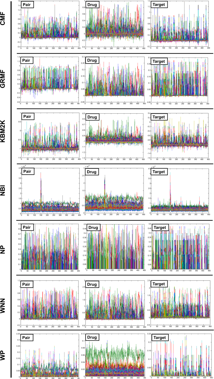
The different cross-validation settings: 1: Pair (DTI)- involves drug-target pairs from the interaction matrix Y to use as the test set, 2: Drug- is the setting where entire drug profiles are shown and 3: Target- entire target profiles. The CV settings for S1, S2, and S3 are provided on the X-axis while the Y-axis represents the standard deviation (SD) of all the employed techniques.
-
(ii)
In the ion channels (IC) and enzymes (E) data sets, the performance of the Weighted Profile is better than the Nearest Profile. This is due to the reason that IC and E data sets are larger than non-redundant (NR) and G-Protein Coupled Receptor (GPCR) counterparts having a large number of neighbors. Therefore, interactions can be deduced more accurately (Fig. 4).

Drug prediction case (Drug)
Ongoing from the drug-target interaction CV setting to the Drug CV setting, it was observed that the results in Fig. 4 were more interesting than the Drug-target interaction. Usually, it is more difficult to predict interactions for the drugs or targets which are unknown in the test sets. This is different from the Drug-target interaction where the drug or target interaction profiles are partially missing out.
The performance of WGRMF is best, followed by the CMF. Therefore, the Matrix Factorization method is again performing well in general. The WGRMF has done well than the CMF under Drug setting because of its graph regularization terms. This also expresses the benefits of manifold learnings while it is an informative locale.
RLS-WNN, which is based upon the network similarities also provides a useful prediction performance. The reasonable performance of RLS-WNN is due to its preprocessing procedure which strengthens its learning progression by inferring to the temporary profiles for the missing drugs. The network similarity in RLS-WNN is calculated by the GIP kernels which can be used in the algorithm later on. Logically, temporary profiles are indeed better for calculating network similarity than the initially empty profiles of the missing drugs, which underlines the significance of preprocessing procedures like WNN when the inclusion of a network similarity in training the classifiers is intended.
Target prediction case (Target)
As projected, the AUPR (Area Under the Precision-Recall) results of the Target settings are relatively lower than the S1 setting but are gradually higher than those of the results obtained under drug-target interaction settings. Methods including Matrix Factorization are usually better in drug cases. From here, we conclude that the target genomic sequence similarities are extremely better even than the similarities of drugs’ chemical structures. The performance of WGRMF is better even than the CMF due to the involvement of graph regularization terms. However, RLS-WNN has an average performance. As for NBI, similar to the Drugs’ cases and Drug-target interactions, It is not capable to outperform the Nearest Profile, baseline methods, and Weighted Profiles. Therefore, it is concluded that the best choice for the prediction of DTIs is network-based methods as shown in Fig. 4; for more information (Supplementary Data).
Discussion
Many computational techniques are involved in drug repositioning which is used in various conditions, depending on the existing knowledge about the concerned disease or adverse condition. Using these methods, we have generated an outline of DTI prediction, which is an important aspect of the drug discovery process. Many web servers have been developed to deal with this work for practitioners, intending to perform this work on a universal scale.
Generally, in the prediction of DTIs, the best method reported is the Matrix Factorization method. In addition to this, the manifold assumption is that the point lies on or near to the low dimensional manifold90,91,92 are more successful for the improvement of DTIs’ prediction performance (as demonstrated by WGRMF). It is essential to state that the RLS-WNN method did not compete with the Matrix Factorization method in the DTIs prediction but an added advantage is the faster algorithm (RLS-WNN). However, when someone wants to predict DTIs, it is beneficial to obtain the primary predictions by RLS-WNN first. It is also highlighted that if the data sets are larger, then the BLMs (Bipartite local models) are the best to be considered as they are proved to be faster and efficient.
While considering the network-based method (NBI), it did not perform well in comparison to other methods which may be due to the properties of DTIs networks that are not satisfactory to deal with network-based methods. Examples related to the interactions of drugs or targets present in the network are very less or there may be the presence of undiscovered interactions present in the noninteracting groups (which may have a negative influence upon the obtained prediction). Moreover, their performance in the prediction of new interactions for orphan drugs (previously unknown interactions) is not well discovered. However, this problem becomes more complex when attempts are being made to predict new interactions for the orphan targets as well; this is because of the indirect network path between the orphan drug and its target which gives a low prediction score; for more information (Supplementary Data).
Conclusion
Alternatively, network-based methods still have a significant role in predicting DTIs. For example, the NRWRH80, the generation of a heterogeneous network is a prominent idea for performing DTIs prediction. By improving the heterogeneous network with more data (i.e. addition of more drug-target pairwise similarities) can help the network-based methods to solve the issues occurring in DTIs prediction for orphan drugs or targets up to some extents. It is also helpful to be inspired from the previous effort on generating functional linkage network (FLNs). FLNs are functionally linked networks between genes that have been used successfully in genes-related functions and disease research. To construct FLN, it requires the information collected from various heterogeneous resources of varying classes and comprehensiveness that may highly correlate with each other. Such understanding in creating FLNs can be delivered to the generation of heterogeneous DTI networks on which network-based methods can be applied for new DTIs prediction with greater precision and accuracy.
In the present work, we have started with a brief description of the data that we required for the drug-DTI prediction and also showed some examples that could be used for its prediction. An outline of different methods is given that are trained with the available data. After this, we have performed an empirical comparison between the methods which are best in their respective category, to illustrate their prediction performances under different situations. At last, a compiled list of all the possibilities was provided for further enhancement of the prediction performance.
According to data, the datasets are binary in nature, i.e. given an interaction matrix Y (where Yij = 1 if the drug and target interact with each other, if there is no interaction Yij = 0); that creates another possibility. Some of the interactions where Yij = 0 have not yet been discovered, which may create a problem in the training process for various classifiers. Besides, there is another possibility that in a real situation, the drug-target pairs having binding energies, showing variations over a wide range of the spectrum (interactions are not binary on/off). Some data sets having continuous values representing drug-target binding energies (as opposed to distinct 0 and 1 values). For that reason, using such continuous-valued data sets is more useful because it represents the actual situation than the binary sets in a better way which has been used earlier in the DTI’s prediction extensively.
Future direction
The type of work mentioned above particularly focuses on the target proteins, but there is another type of target which is the noncoding RNAs (ncRNAs), and the drugs which are successfully developed. These are the RNAs that are not protein-coding, and they contain subcategories which include microRNAs (miRNAs), long coding RNAs (lcRNA) and Intronic RNAs (iRNA) among several others. A few examples are the use of miRNAs to treat the Hepatitis C virus and Alport nephropathy. The behavior and mechanism of each of the ncRNAs are quite. Research on chemogenomic methods for prediction of ncRNAs is likely to continue for the next several years with contributions involving deep learning concepts, Multiview learning and possibly unprecedented clever features for representing drugs or targets. Therefore, it leads to different opportunities and challenges, all of which are discussed with examples in the recent reports regarding DTIs.
Data availability
The way we want to predict the new DTI is completely different from the existing training data. The data which represents the drug and the target involved in the interaction is also needed for this purpose. The overall workflow for the prediction of new DTIs is graphically produced (Fig. 1). Interaction data were retrieved from different sources. Drugs data were retrieved from Rcpi, PyDPI, and Open Babel. Targets data were retrieved from Gene Ontology (GO) information, gene expression profiles, gene sequence, disease associations, and protein-protein interaction (PPI) network information; for more information (Supplementary Data). All data generated and analyzed during this study are included in this article. The proposed DTI (Dataset, Statistical Metrics, Confidence Interval & Benchmark Evaluation Results) is freely accessible at http://weislab.com/WeiDOCK/?page=DTI.
The provided data includes dataset files (.txt format), metrics files (.mat format), statistical metrics (.mat format), confidence intervals (.mat format), benchmark evaluation results (.mat format), and scripts for executing this DIT Model (.py format).
References
Wen, M. et al. Deep-learning-based drug–target interaction prediction. Journal of proteome research 16, 1401–1409 (2017).
Chen, X. et al. Drug–target interaction prediction: databases, web servers and computational models. Briefings in bioinformatics 17, 696–712 (2015).
Kaushik, A. C. & Sahi, S. Biological complexity: ant colony meta-heuristic optimization algorithm for protein folding. Neural Computing and Applications, 28(11), 3385–3391 (2017).
Ashburn, T. T. & Thor, K. B. Drug repositioning: identifying and developing new uses for existing drugs. Nature reviews Drug discovery 3, 673 (2004).
Ding, H., Takigawa, I., Mamitsuka, H. & Zhu, S. Similarity-based machine learning methods for predicting drug–target interactions: a brief review. Briefings in bioinformatics 15, 734–747 (2013).
Novac, N. Challenges and opportunities of drug repositioning. Trends in pharmacological sciences 34, 267–272 (2013).
Wu, Z., Wang, Y. & Chen, L. Network-based drug repositioning. Molecular BioSystems 9, 1268–1281 (2013).
Wu, C., Gudivada, R. C., Aronow, B. J. & Jegga, A. G. Computational drug repositioning through heterogeneous network clustering. BMC systems biology 7, S6 (2013).
Vanunu, O., Magger, O., Ruppin, E., Shlomi, T. & Sharan, R. Associating genes and protein complexes with disease via network propagation. PLoS computational biology 6, e1000641 (2010).
Hearst, M. A. In Proceedings of the 37th annual meeting of the Association for Computational Linguistics on Computational Linguistics. 3–10 (Association for Computational Linguistics).
Xue, H., Li, J., Xie, H. & Wang, Y. Review of drug repositioning approaches and resources. International journal of biological sciences 14, 1232 (2018).
Frantz, S. (Nature Publishing Group, 2005).
McLean, S. R. et al. Imatinib binding and cKIT inhibition is abrogated by the cKIT kinase domain I missense mutation Val654Ala. Molecular cancer therapeutics 4, 2008–2015 (2005).
Pepin, J., Guern, C., Milord, F. & Schechter, P. Difluoromethylornithine for arseno-resistant Trypanosoma brucei gambiense sleeping sickness. The Lancet 330, 1431–1433 (1987).
Chong, C. R., Chen, X., Shi, L., Liu, J. O. & Sullivan, D. J. Jr A clinical drug library screen identifies astemizole as an antimalarial agent. Nature chemical biology 2, 415 (2006).
Miguel, D. C., Yokoyama-Yasunaka, J. K., Andreoli, W. K., Mortara, R. A. & Uliana, S. R. Tamoxifen is effective against Leishmania and induces a rapid alkalinization of parasitophorous vacuoles harbouring Leishmania (Leishmania) amazonensis amastigotes. Journal of Antimicrobial Chemotherapy 60, 526–534 (2007).
Chow, W. A., Jiang, C. & Guan, M. Anti-HIV drugs for cancer therapeutics: back to the future? The lancet oncology 10, 61–71 (2009).
Gloeckner, C. et al. Repositioning of an existing drug for the neglected tropical disease Onchocerciasis. Proceedings of the National Academy of Sciences 107, 3424–3429 (2010).
Aronson, J. Old drugs–new uses. British journal of clinical pharmacology 64, 563–565 (2007).
Wang, Y. et al. Pubchem bioassay: 2017 update. Nucleic acids research 45, D955–D963 (2016).
Yao, L., Evans, J. A. & Rzhetsky, A. Novel opportunities for computational biology and sociology in drug discovery: Corrected paper. Trends in biotechnology 28, 161–170 (2010).
Keiser, M. J. et al. Predicting new molecular targets for known drugs. Nature 462, 175 (2009).
Goodsell, D. S., Morris, G. M. & Olson, A. J. Automated docking of flexible ligands: applications of AutoDock. Journal of molecular recognition 9, 1–5 (1996).
Pérez, A. et al. Refinement of the AMBER force field for nucleic acids: improving the description of α/γ conformers. Biophysical journal 92, 3817–3829 (2007).
Yang, S. et al. cmFSM: a scalable CPU-MIC coordinated drug-finding tool by frequent subgraph mining. BMC bioinformatics 19, 98 (2018).
Cheng, Q. et al. In 2015 15th IEEE/ACM International Symposium on Cluster, Cloud and Grid Computing. 725–728 (IEEE).
Cui, Y. et al. mSNP: A massively parallel algorithm for large-scale SNP detection. IEEE Transactions on Parallel and Distributed Systems 29, 2557–2567 (2018).
Kaushik, A. C. et al. A-CaMP: a tool for anti-cancer and antimicrobial peptide generation. Journal of Biomolecular Structure and Dynamics, 1–9 (2020).
Dong, D., Su, W., Shi, W., Zou, Q. & Peng, S. VCSRA: A fast and accurate multiple sequence alignment algorithm with a high degree of parallelism. Journal of genetics and genomics= Yi chuan xue bao 45, 407 (2018).
Schellhammer, I. & Rarey, M. FlexX-Scan: Fast, structure-based virtual screening. PROTEINS: Structure, Function, and Bioinformatics 57, 504–517 (2004).
Johnson, M. A. & Maggiora, G. M. Concepts and applications of molecular similarity. (Wiley, 1990).
Keiser, M. J. et al. Relating protein pharmacology by ligand chemistry. Nature biotechnology 25, 197 (2007).
Jacob, L. & Vert, J.-P. Protein-ligand interaction prediction: an improved chemogenomics approach. Bioinformatics 24, 2149–2156 (2008).
Li, H. et al. TarFisDock: a web server for identifying drug targets with docking approach. Nucleic acids research 34, W219–W224 (2006).
Cheng, A. C. et al. Structure-based maximal affinity model predicts small-molecule druggability. Nature biotechnology 25, 71 (2007).
Kaushik, A. C. & Sahi, S. HOGPred: artificial neural network-based model for orphan GPCRs. Neural Computing and Applications, 29(4), 985–992 (2018).
Kaushik, A. C. et al. Deciphering the biochemical pathway and pharmacokinetic study of amyloid βeta-42 with superparamagnetic iron oxide nanoparticles (SPIONS) using systems biology approach. Molecular neurobiology, 55(4), 3224–3236 (2018).
Yıldırım, M. A., Goh, K.-I., Cusick, M. E., Barabási, A.-L. & Vidal, M. Drug—target network. Nature biotechnology 25, 1119 (2007).
Opella, S. J. Structure determination of membrane proteins by nuclear magnetic resonance spectroscopy. Annual Review of Analytical Chemistry 6, 305–328 (2013).
Yamanishi, Y., Araki, M., Gutteridge, A., Honda, W. & Kanehisa, M. Prediction of drug–target interaction networks from the integration of chemical and genomic spaces. Bioinformatics 24, i232–i240 (2008).
Bredel, M. & Jacoby, E. Chemogenomics: an emerging strategy for rapid target and drug discovery. Nature Reviews Genetics 5, 262 (2004).
Mousavian, Z. & Masoudi-Nejad, A. Drug–target interaction prediction via chemogenomic space: learning-based methods. Expert opinion on drug metabolism & toxicology 10, 1273–1287 (2014).
Pahikkala, T. et al. Toward more realistic drug–target interaction predictions. Briefings in bioinformatics 16, 325–337 (2014).
Yamanishi, Y. et al. DINIES: drug–target interaction network inference engine based on supervised analysis. Nucleic acids research 42, W39–W45 (2014).
Kanehisa, M., Goto, S., Sato, Y., Furumichi, M. & Tanabe, M. KEGG for integration and interpretation of large-scale molecular data sets. Nucleic acids research 40, D109–D114 (2011).
Knox, C. et al. DrugBank 3.0: a comprehensive resource for’omics’ research on drugs: Nucleic Acids Res. Database issue) D1035-41 (2011).
Gaulton, A. et al. ChEMBL: a large-scale bioactivity database for drug discovery. Nucleic acids research 40, D1100–D1107 (2011).
Kuhn, M. et al. STITCH 4: integration of protein–chemical interactions with user data. Nucleic acids research 42, D401–D407 (2013).
Mehmood, A., Kaushik, A. C. & Wei, D. Q. Prediction and validation of potent peptides against herpes simplex virus type 1 via immunoinformatic and systems biology approach. Chem. Biol. Drug Des 94, 1868–1883 (2019).
van Laarhoven, T., Nabuurs, S. B. & Marchiori, E. Gaussian interaction profile kernels for predicting drug–target interaction. Bioinformatics 27, 3036–3043 (2011).
Van Laarhoven, T. & Marchiori, E. Predicting drug-target interactions for new drug compounds using a weighted nearest neighbor profile. PloS one 8, e66952 (2013).
Cheng, F. et al. Prediction of drug-target interactions and drug repositioning via network-based inference. PLoS computational biology 8, e1002503 (2012).
Gönen, M. Predicting drug–target interactions from chemical and genomic kernels using Bayesian matrix factorization. Bioinformatics 28, 2304–2310 (2012).
Zheng, X., Ding, H., Mamitsuka, H. & Zhu, S. In Proceedings of the 19th ACM SIGKDD international conference on Knowledge discovery and data mining. 1025–1033 (ACM).
Ezzat, A., Zhao, P., Wu, M., Li, X.-L. & Kwoh, C.-K. Drug-target interaction prediction with graph regularized matrix factorization. IEEE/ACM Transactions on Computational Biology and Bioinformatics (TCBB) 14, 646–656 (2017).
Gu, Q., Zhou, J. & Ding, C. In Proceedings of the 2010 SIAM international conference on data mining. 199–210 (SIAM).
Shang, F., Jiao, L. & Wang, F. Graph dual regularization non-negative matrix factorization for co-clustering. Pattern Recognition 45, 2237–2250 (2012).
Weininger, D. SMILES, a chemical language and information system. 1. Introduction to methodology and encoding rules. Journal of chemical information and computer sciences 28, 31–36 (1988).
Kuhn, M., Campillos, M., Letunic, I., Jensen, L. J. & Bork, P. A side effect resource to capture phenotypic effects of drugs. Molecular systems biology 6 (2010).
Skrbo, A., Begović, B. & Skrbo, S. Classification of drugs using the ATC system (Anatomic, Therapeutic, Chemical Classification) and the latest changes. Medicinski arhiv 58, 138–141 (2004).
Lamb, J. The Connectivity Map: a new tool for biomedical research. Nature reviews cancer 7, 54 (2007).
Cao, D.-S., Xiao, N., Xu, Q.-S. & Chen, A. F. Rcpi: R/Bioconductor package to generate various descriptors of proteins, compounds and their interactions. Bioinformatics 31, 279–281 (2014).
Cao, D.-S. et al. (ACS Publications, 2013).
O’Boyle, N. M. et al. Open Babel: An open chemical toolbox. Journal of cheminformatics 3, 33 (2011).
Jain, E. et al. Infrastructure for the life sciences: design and implementation of the UniProt website. BMC bioinformatics 10, 136 (2009).
Ashburner, M. et al. Gene ontology: tool for the unification of biology. Nature genetics 25, 25 (2000).
Emig, D. et al. Drug target prediction and repositioning using an integrated network-based approach. PLoS One 8, e60618 (2013).
Zong, N., Kim, H., Ngo, V. & Harismendy, O. Deep mining heterogeneous networks of biomedical linked data to predict novel drug–target associations. Bioinformatics 33, 2337–2344 (2017).
Cannataro, M., Guzzi, P. H. & Veltri, P. Protein-to-protein interactions: Technologies, databases, and algorithms. ACM Computing Surveys (CSUR) 43, 1 (2010).
Klingström, T. & Plewczynski, D. Protein–protein interaction and pathway databases, a graphical review. Briefings in bioinformatics 12, 702–713 (2010).
Zhang, P. et al. A protein network descriptor server and its use in studying protein, disease, metabolic and drug targeted networks. Briefings in bioinformatics 18, 1057–1070 (2016).
Shi, J.-Y. & Yiu, S.-M. In 2015 IEEE International Conference on Bioinformatics and Biomedicine (BIBM). 1636–1641 (IEEE).
Bleakley, K. & Yamanishi, Y. Supervised prediction of drug–target interactions using bipartite local models. Bioinformatics 25, 2397–2403 (2009).
Xia, Z., Zhou, X., Sun, Y. & Wu, L. In The Third International Symposium on Optimization and Systems Biology. 123–131 (Citeseer).
Mei, J.-P., Kwoh, C.-K., Yang, P., Li, X.-L. & Zheng, J. Drug–target interaction prediction by learning from local information and neighbors. Bioinformatics 29, 238–245 (2012).
Cheng, F., Zhou, Y., Li, W., Liu, G. & Tang, Y. Prediction of chemical-protein interactions network with weighted network-based inference method. PloS one 7, e41064 (2012).
Wang, W., Yang, S. & Li, J. In Biocomputing 2013 53-64 (World Scientific, 2013).
Chen, X., Liu, M.-X. & Yan, G.-Y. Drug–target interaction prediction by random walk on the heterogeneous network. Molecular BioSystems 8, 1970–1978 (2012).
Fakhraei, S., Huang, B., Raschid, L. & Getoor, L. Network-based drug-target interaction prediction with probabilistic soft logic. IEEE/ACM Transactions on Computational Biology and Bioinformatics (TCBB) 11, 775–787 (2014).
Ba-Alawi, W., Soufan, O., Essack, M., Kalnis, P. & Bajic, V. B. DASPfind: new efficient method to predict drug–target interactions. Journal of cheminformatics 8, 15 (2016).
Cobanoglu, M. C., Liu, C., Hu, F., Oltvai, Z. N. & Bahar, I. Predicting drug–target interactions using probabilistic matrix factorization. Journal of chemical information and modeling 53, 3399–3409 (2013).
Liu, Y., Wu, M., Miao, C., Zhao, P. & Li, X.-L. Neighborhood regularized logistic matrix factorization for drug-target interaction prediction. PLoS computational biology 12, e1004760 (2016).
Hao, M., Bryant, S. H. & Wang, Y. Predicting drug-target interactions by dual-network integrated logistic matrix factorization. Scientific reports 7, 40376 (2017).
He, Z. et al. Predicting drug-target interaction networks based on functional groups and biological features. PloS one 5, e9603 (2010).
Yu, H. et al. A systematic prediction of multiple drug-target interactions from chemical, genomic, and pharmacological data. PloS one 7, e37608 (2012).
Xiao, X., Min, J.-L., Wang, P. & Chou, K.-C. iGPCR-Drug: A web server for predicting interaction between GPCRs and drugs in cellular networking. PloS one 8, e72234 (2013).
Ezzat, A., Wu, M., Li, X.-L. & Kwoh, C.-K. Drug-target interaction prediction via class imbalance-aware ensemble learning. BMC bioinformatics 17, 509 (2016).
Ezzat, A., Wu, M., Li, X.-L. & Kwoh, C.-K. Drug-target interaction prediction using ensemble learning and dimensionality reduction. Methods 129, 81–88 (2017).
Perlman, L., Gottlieb, A., Atias, N., Ruppin, E. & Sharan, R. Combining drug and gene similarity measures for drug-target elucidation. Journal of computational biology 18, 133–145 (2011).
Tenenbaum, J. B., De Silva, V. & Langford, J. C. A global geometric framework for nonlinear dimensionality reduction. science 290, 2319–2323 (2000).
Roweis, S. T. & Saul, L. K. Nonlinear dimensionality reduction by locally linear embedding. science 290, 2323–2326 (2000).
Belkin, M. & Niyogi, P. In Advances in neural information processing systems. 585–591.
Raymond, R. & Kashima, H. In Joint european conference on machine learning and knowledge discovery in databases. 131–147 (Springer).
Peng, H., Long, F. & Ding, C. Feature selection based on mutual information: criteria of max-dependency, max-relevance, and min-redundancy. IEEE Transactions on Pattern Analysis & Machine Intelligence, 1226–1238 (2005).
De Jong, S. SIMPLS: an alternative approach to partial least squares regression. Chemometrics and intelligent laboratory systems 18, 251–263 (1993).
Wang, L. et al. Rfdt: A rotation forest-based predictor for predicting drug-target interactions using drug structure and protein sequence information. Current Protein and Peptide Science 19, 445–454 (2018).
Zhang, C.-X. & Zhang, J.-S. A variant of Rotation Forest for constructing ensemble classifiers. Pattern Analysis and Applications 13, 59–77 (2010).
Zhou, Z.-H. Ensemble methods: foundations and algorithms. (Chapman and Hall/CRC, 2012).
Meng, F.-R., You, Z.-H., Chen, X., Zhou, Y. & An, J.-Y. Prediction of drug–target interaction networks from the integration of protein sequences and drug chemical structures. Molecules 22, 1119 (2017).
Tipping, M. E. Sparse Bayesian learning and the relevance vector machine. Journal of machine learning research 1, 211–244 (2001).
Huang, Y.-A., You, Z.-H. & Chen, X. A systematic prediction of drug-target interactions using molecular fingerprints and protein sequences. Current Protein and Peptide Science 19, 468–478 (2018).
Yamanishi, Y., Pauwels, E., Saigo, H. & Stoven, V. Extracting sets of chemical substructures and protein domains governing drug-target interactions. Journal of chemical information and modeling 51, 1183–1194 (2011).
Finn, R., Mistry, J., Tate, J., Coggill, P. & Heger, A. Pfam: the protein families database. Nuclei. Acids Re (2014).
Tabei, Y. & Yamanishi, Y. Scalable prediction of compound-protein interactions using minwise hashing. BMC systems biology 7, S3 (2013).
Acknowledgements
The simulations in this work were supported by the Center for High-Performance Computing, Shanghai Jiao Tong University. Thanks to Prof. Cheng-Tang Pan and Yow-Ling Shiue for their support to improve manuscript visibility. This work was supported by the Key Research Area Grant 2016YFA0501703 of the Ministry of Science and Technology of China, the National Natural Science Foundation of China (Contract no. 61832019 and 61503244), the State Key Lab of Microbial Metabolism, and the Joint Research Funds for Medical and Engineering and Scientific Research at Shanghai Jiao Tong University (YG2017ZD14). These funding sources have no role in the writing of the manuscript or the decision to submit it for publication.
Author information
Authors and Affiliations
Contributions
A.C.K. and D.Q.W. designed the experiments. A.C.K. and D.Q.W. computationally scripted DTI and assisted in writing the manuscript. D.Q.W. and A.C.K. analyzed the data and wrote the manuscript. A.C.K., D.Q.W., X.F.D., and A.M. read the manuscript and advised on the method development. All authors have approved the final version of the manuscript.
Corresponding authors
Ethics declarations
Competing interests
The authors declare no competing interests.
Additional information
Publisher’s note Springer Nature remains neutral with regard to jurisdictional claims in published maps and institutional affiliations.
Supplementary information
Rights and permissions
Open Access This article is licensed under a Creative Commons Attribution 4.0 International License, which permits use, sharing, adaptation, distribution and reproduction in any medium or format, as long as you give appropriate credit to the original author(s) and the source, provide a link to the Creative Commons license, and indicate if changes were made. The images or other third party material in this article are included in the article’s Creative Commons license, unless indicated otherwise in a credit line to the material. If material is not included in the article’s Creative Commons license and your intended use is not permitted by statutory regulation or exceeds the permitted use, you will need to obtain permission directly from the copyright holder. To view a copy of this license, visit http://creativecommons.org/licenses/by/4.0/.
About this article

Cite this article
Kaushik, A.C., Mehmood, A., Dai, X. et al. A comparative chemogenic analysis for predicting Drug-Target Pair via Machine Learning Approaches. Sci Rep 10, 6870 (2020). https://doi.org/10.1038/s41598-020-63842-7
Received:
Accepted:
Published:
DOI: https://doi.org/10.1038/s41598-020-63842-7
This article is cited by
-
Drug repurposing and prediction of multiple interaction types via graph embedding
BMC Bioinformatics (2023)
-
DEDTI versus IEDTI: efficient and predictive models of drug-target interactions
Scientific Reports (2023)
-
Novel drug-target interactions via link prediction and network embedding
BMC Bioinformatics (2022)
Comments
By submitting a comment you agree to abide by our Terms and Community Guidelines. If you find something abusive or that does not comply with our terms or guidelines please flag it as inappropriate.
