
Abstract
Surface soil moisture (SSM) is an important variable in drought monitoring, floods predicting, weather forecasting, etc. and plays a critical role in water and heat exchanges between land and atmosphere. SSM products from L-band observations, such as the Soil Moisture Active Passive (SMAP) Mission, have proven to be optimal global estimations. Although X-band has a lower sensitivity to soil moisture than that of L-band, Chinese FengYun-3 series satellites (FY-3A/B/C/D) have provided sustainable and daily multiple SSM products from X-band since 2008. This research developed a new global SSM product (NNsm-FY) from FY-3B MWRI from 2010 to 2019, transferred high accuracy of SMAP L-band to FY-3B X-band. The NNsm-FY shows good agreement with in-situ observations and SMAP product and has a higher accuracy than that of official FY-3B product. With this new dataset, Chinese FY-3 satellites may play a larger role and provide opportunities of sustainable and longer-term soil moisture data record for hydrological study.
Background & Summary
Surface soil moisture (SSM) is essential for agriculture, ecosystem, weather, climate system and human health1,2,3,4. SSM is a boundary condition, affecting the evapotranspiration and infiltration in water cycle, as well as the latent and sensible heat fluxes in land surface energy balance5,6,7,8,9. Soil moisture is necessary for crop growth and yield, and soil moisture plays important role in monitoring disaster (e.g., drought, flood, landslide etc.)10,11,12 and climate extremes (e.g., heatwave)13,14. Soil information can help improve weather forecasting accuracy and model performance when using soil moisture observed by satellites into land surface model15,16,17. Long-term and spatio-temporally consistent SSM datasets are therefore necessary for those applications and scientific researches18,19.
Microwave remote sensing has proven successful for providing spatial and temporal distribution of global soil moisture from satellite missions, especially L band passive sensors in recent years. C/X/K band sensors (SSM/I (Special Sensor Microwave/Imager), AMSR-E/AMSR2 (Advanced Microwave Scanning Radiometer), MWRI etc.20,21) provide 40 years SSM observations at sensing depth of ~1 cm, with more uncertainties due to vegetation effects compared with L band. In contrast, L band radiometers (SMOS (Soil Moisture and Ocean Salinity) and SMAP) provide only 14 years and 8 years SSM products with higher accuracy at sensing depth of ~5 cm, with more penetration into vegetation and less opaque of atmosphere22,23.
To meet more application requirements for long-term datasets, there are generally two strategies: 1) The first strategy is SSM retrieval with one consistent algorithm, which requires inter-calibrated microwave observations. Different methods have been explored, including the regression method24, the neural network (NN) method25,26, the land parameter retrieval model (LPRM), and the recent multi-channel collaborative algorithm (MCCA)27, etc. 2) The second strategy is to blend multi-satellite products. Owe28 developed a dataset dating back to 2007 by applying LPRM to the entire brightness temperature (TB) observed by C- and X-bands sensors. Then, Liu29,30 combined products from active and passive microwave sensors by rescaling active and passive products to a reference land surface model data using a cumulative distribution function (CDF) matching approach. On the basis of above works, Gruber31 proposed a triple collocation analysis (TCA)-based method for merging soil moisture taking into account the error characteristics of the individual active and passive datasets, forming the basis of Climate Change Initiative soil moisture (CCIsm) product version v03.x and higher. SMOPS32 (soil moisture operational product system) provides a daily global SSM product with high spatial coverage (2017.03-present) that merged soil moisture retrievals from multiple satellites.
CCIsm33,34,35,36 is a publicly available and widely used long-term soil moisture dataset. While CCIsm has sufficient record length (from 1978.11 to present) for climatological studies, it depends on numerous sensor specifications and CDF matching reduces inter-annual variability and climatological trends. It is found that the accuracy of CCIsm depends on regions and seasons, and the accuracy could be further improved through blending more SSM products. To be noted, the CCIsm only blends the FY-3B observations from June 2011 to August 2019. We developed a NN method extending L band (SMOS or SMAP) benefits to previous C/X band AMSR-E/AMSR2 data, and then released a nearly 20 years long-term soil moisture product37,38 (NNsm-AMSR), with high accuracy similar to SMAP but greater spatial coverage than SMOS and SMAP. Unfortunately, NNsm-AMSR has a temporal gap of 9 months due to data gaps between AMSR-E and AMSR2 sensors, which limits its applications. On the other hand, MWRI onboard Chinese FY-3 satellites has almost the same frequencies configuration with AMSR-E/AMSR2 except C-band, and the FY-3 (B/C/D) data are available since 2010. The development of FY-3 SSM products can be an important input for future blended SSM products.
This research developed an SSM product (named as NNsm-FY) at 36 km resolution from 2010 to 2019 by transfering high accuracy of SMAP L-band SSM to X-band MWRI of FY-3B. Figure 1 shows the scheme of the NNsm-FY dataset development. Validation against in situ data from representative networks demonstrate that the NNsm-FY matches well with in situ SSM, with similar accuracy to SMAP (~0.04 m3/m3). This dataset provides a new soil moisture product of Chinese FY-3 with high accuracy, and fills in the gap (2011.11–2012.06) between the effective end of AMSR-E and beginning of the AMSR2, such as a previously developed long term dataset NNsm-AMSR39, and intends to provide opportunities for sustainable and longer-term soil moisture for hydrological or climate change study at global or regional scale.

Flow chart of soil moisture retrieval of NNsm-FY dataset.
Methods
In our research, we used two kinds of data. SMAP level 3 soil moisture product (SMAPL3sm, Version 6), available at website of National Snow and Ice Data Center (NSIDC, https://nsidc.org/data/smap), are in a global cylindrical 36 km Equal-Area Scalable Earth Grid, Version 2.0 (EASE-Grid 2.0), with size of 406 rows × 964 columns. TBs of FY-3B MWRI are re-calibration level 1 swath data, provided by National Satellite Meteorological Center (NSMC). And the footprint sizes of MWRI 10.65 GHz, 18.7 GHz, 23.8 GHz, 36.5 GHz, 89 GHz are 51 km × 58 km, 30 km × 50 km, 27 km × 45 km, 18 km × 30 km and 18 km × 30 km. Table 1 summarizes the data used, their spatial resolutions, and provenance.
A soil moisture retrieval model was developed based on artificial neural network (ANN), which is a modified version of method developed by Yao37,39. As shown in Fig. 1, the NNsm-FY dataset was generated with three steps:(1) data pre-processing and data matching, (2) training of soil moisture ANN model, (3) retrieval and validation of NNsm-FY dataset.
Data Pre-processing
To match FY-3B TBs with SMAPL3sm, FY-3B TBs are firstly resampled to 36 km. We use the “drop in the bucket” method to resample FY-3B L1 swath data to 36 km EASE-Grid format. All swath data that fall within a 36 km grid cell are averaged together. Microwave vegetation index(MVI), proposed by Shi40, is an indicator of effect of vegetation in soil moisture retrieval. MVI is calculated by TBs of two bands, and the formula is as follows:
Training of soil moisture ANN model
The training is implemented in Matlab R2018b version. Cascade-forward neural network is selected as the training model, with “hiddenSizes” being 10, “Training function” being “trainlm (Levenberg-Marquardt)”. Mean squared error (mse) is used to evaluate the performance of the neural network. In the training period from 2015 to 2017, the training target is SMAPL3sm, and the Input data are matched FY-3 TBs from 10 GHz to 36.5 GHz and MVI derived from FY-3 TBs. The training dataset doesn’t include the frozen condition, cause the SMAPL3sm has no value when soil is frozen.
The ANN model is trained to learn the relationship between the input TBs related variables and the target SMAPL3sm. The model is trained separately for each grid cell in Matlab R2018b version. To reduce the impact of temperature in soil moisture model, FY-3 TBs at 2:00 o’clock and SMAPL3sm at 06:00 o’clock are selected. From 2015 to 2017, spatial-temporal matched FY-3B data and SMAP data form the training dataset.
Matlab randomly divide the training dataset into 3 kinds of samples: 70% training samples, 15% validation samples and 15% testing samples. The network is trained and adjusted according to its error of multiple train epochs with training samples. The validation samples are used to halt training when the network stops improving. The test sample provide an independent measure of network performance during and after training.
Retrieval of NNsm-FY for each grid cell
After establishing the ANN relationship model between the input and the target for each grid cell, the model is applied with inputting pre-processed FY-3B TBs and MVI at the corresponding 36 km grid cell from 2010 to 2019. The retrieval is implemented using one year’s daily data over one grid cell, and the global daily soil moisture from 2010 to 2019 are obtained finally.
Data Records
The data records41 contain global daily soil moisture data with a spatial resolution of 36 km, in unit of m3/m3, from November 2010 to July 2019. These data are stored in NetCDF format with one file per day, defined by two dimensions (lat, lon, respectively representing latitude and longitude) and a variable soil moisture (soil_moisture). The file name is “NNsm-FY-yyyyddd.nc”, where “yyyy” stands for year and “ddd” stands for Julian date. For example, “2019001.nc” contains the global soil moisture distribution on the first day of 2019. This dataset is freely available from National Tibetan Plateau Data Center (TPDC, http://data.tpdc.ac.cn/).
Naming convention:
NNsm-FY-yyyyddd.nc
Variable: soil_moisture = volumetric soil moisture [m3/m3]
Technical Validation
Validation is critical for providing accurate product before widely usage. The NNsm-FY dataset was validated at different spatio-temporal scales. Before validation, the training results were evaluated by comparing with training target. The NNsm-FY dataset was firstly validated using in-situ observations. Then the performance of NNsm-FY was compared with that of FY-3B official soil moisture product (FY-sm) and ERA5 soil moisture. We previously developed a soil moisture product called NNsm_AMSR (2002–2011,2012–2020) using similar method with SMAPL3sm and AMSR-E/AMSR2 TB. Finally, the homogeneity of NNsm-FY and NNsm_AMSR was verified. For evaluation against in situ observations and other SSM products, we used the correlation coefficient (CC), root mean square error (RMSE), bias, unbiased RMSE (ubRMSE) for statistical results.
Evaluation of training results
To demonstrate the reliable of soil moisture ANN model, the relationship between the training results with training target SMAPL3sm is shown in Fig. 2, in terms of CC, RMSE and relative error at each grid cell over the training period. Traning results has high CC (>0.8) with the target SMAPL3sm globally, except for regions of equatorial rainforest and forest at high latitude such as part of Russia. Statistically, 57 percent of RMSEs over global land are below 0.03 m3/m3, and 29 percent of RMSEs is between 0.03 m3/m3 and 0.05 m3/m3. The high CC and low RMSE indicate that the input and the target of the model has a good correlation, and the trained result has a good agreement with the target.

Statistical map between training result and SMAPL3sm over training period (2015–2017): (a) CC, (b) RMSE(m3/m3), (c) Relative error and (d) RMSE distribution at different NDVI interval.
The map of relative error in Fig. 2c shows a different information of error. Statistically, over global land, only 30 percent of relative error is below 10%, 54 percent of relative error is between 10% and 20%. At forest area and tundra area, where the soil moisture is generally high, the relative error is small. At the central part of Eurasia, where the soil moisture is generally low, the relative error is larger. Vegetation effect is an important influence factors in soil moisture retrieval. To test the effect of vegetation on the error level of NNsm-FY, the RMSE distribution between the training result NNsm-FY and the reference target SMAPsm is displayed in Fig. 2d, at different NDVI interval. As a whole the RMSE increases as the NDVI increases. When NDVI is between 0.6 and 0.8, the median of RMSE is 0.034 m3/m3, and when NDVI is greater than 0.8, the median of RMSE is 0.049 m3/m3.
Validation using in situ observations
An ideal in situ validation network should has multiple sampling sites and represent the “truth” within a spatial domain that matching a satellite product grid. We choose both classical “dense” in situ networks with multiple sampling sites for validation, and “sparse” in situ networks with only one or very few sampling sites. These validation networks distribute in different climate regime and land cover in five continents.
-
(1)
Dense validation networks
14 representative in situ dense networks are used for validation, shown in Fig. 3 and Table 2, including: (a) 7 United States Department of Agriculture (USDA) watershed networks42,43, (b) 2 Tibetan Plateau networks, (c) 2 Australian Moisture Monitoring Network (OZNet) networks44, (d) the REMEDHUS network, and (e) 2 African Monsoon Multidisciplinary Analysis (AMMA) networks45. Data of OZNet, REMEDHUS and AMMA sites are provided by International Soil Moisture Network (ISMN) (https://ismn.geo.tuwien.ac.at/) website46,47. As space is limited, time series of bold-face networks are shown in the following figures.
Fig. 3 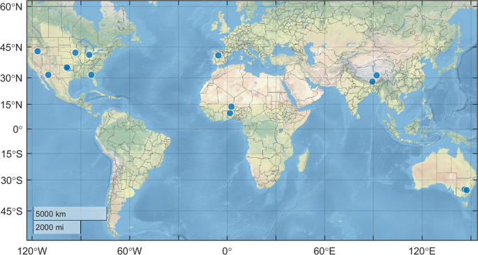
Location of in situ soil moisture validation dense networks.
Table 2 List of validation dense networks. -
(2)
Flux sites

FLUXNET (https://fluxnet.org/) is a global network of micrometeorological tower sites that measure the carbon dioxide, water vapor, and energy between terrestrial ecosystems and the atmosphere. We use 5 flux datasets: (1) FLUXNET201548, the most recent FLUXNET data product, (2) ICOS202049, Warm Winter 2020 ecosystem eddy covariance flux product, (3) ICOSETC202250, (4) AmeriFlux Network (https://ameriflux.lbl.gov/), and (5) TERN, the Terrestrial Ecosystem Research Network(https://portal.tern.org.au/). The half-hour soil moisture observations at 5 cm depth from those sites are used shown in Table 3.
The performance of NNsm-FY over in situ dense networks and Flux sites are shown in time series in Fig. 4 and in a statistical result for an independent validation period (2018–2019) in Table 4.

Time series comparison of the SMAPsm (red dots), NNsm-FY (blue dots) and in situ soil moisture observations (obs-sm in gray lines) for period 2010 to 2019 over in situ networks: (a) Little Washita, (b) Naqu, (c) Yanco, (d) REMEDHUS, (e) Benin.
Figure 4 shows time series comparison of the SMAPsm (red dots), NNsm-FY (blue dots) and in situ soil moisture observations (obs-sm in gray lines). For demonstration, we only show time series for one in situ network in every continent. NNsm-FY can reconstruct the pattern of SMAPsm including magnitude and variability, with a mean CC 0.86. Both NNsm-FY and SMAPsm show good agreement with in situ SSM (obs-sm) at daily time scale, capturing the daily and seasonal dynamics of SSM. For the Little Washita network, there is a slight underestimation during dry period. In Naqu, NNsm-FY has more retrievals than SMAPsm, especially in winter. Over Yanco, in many instances, NNsm-FY overestimates soil moisture associated with precipitation events, together with SMAPsm. For the AMMA-Benin, NNsm-FY overestimates soil moisture at both dry and wet period.
Table 4 and plots in Figs. 5, 6 show statistical results for NNsm-FY and SMAPsm at dense networks and flux sites, at an independent validation period of 2018–2019, for both actual satellite SSM and SSM anomalies. For actual SSM and its anomalies, NNsm-FY generally have a lower accuracy than SMAPsm for most networks, with lower CC and higher ubRMSE. For actual SSM, correlations of NNsm-FY with in situ SSM are slightly lower than that of SMAPsm at dense netwoks, ranging from 0.56 to 0.91 (except 0.35 at South Fork) for NNsm-FY, and ranging from 0.50 to 0.94 for SMAPsm. For SSM anomalies, NNsm-FY performs worse than SMAPsm at most networks in terms of CC. For both NNsm-FY and SMAPsm, SSM anomalies have higher accuracy in terms of ubRMSE. Although the SSM anomalies show lower CC than actual SSM, both products still have relatively strong correlations and high accuracy after removing seasonal cycle.

CC of NNsm-FY and SMAPL3sm against in situ soil moisture at 12 dense validation networks, at an independent validation period (2018–2019), for both actual SSM and SSM anomalies.

Box plots of statistics of NNsm-FY and SMAPsm against in situ soil moisture at an independent validation period (2018–2019), for both actual SSM and SSM anomalies: (a) CC, (b) ubRMSE(m3/m3) at dense networks, (c) CC and (d) ubRMSE(m3/m3) at flux sites.
From Fig. 5 over most sites CC of SSM anomalies are stable or slightly decrease from the CC of actual SSM, both for NNsm-FY and SMAP. Over site South Fork, NNsm-FY performs worse than SMAPsm, and it is more pronounced for SSM anomalies. Over site Naqu and site Kyeamba, NNsm-FY and SMAPsm have similar performance, but CC of NNsm-FY (Anomalies) is lower than CC of SMAP (Anomalies). There are several reasons for the difference of performance between NNsm-FY and SMAPsm. L-band on SMAP has higher sensitivity to soil moisture than high-frequency bands such as X-band,Ku-band and K-band on MWRI/FY-3B; The incident angle of SMAP (40°) is different with incident angle of MWRI/FY-3B (53°). Studies have shown that performance of soil moisture estimations is better at intermediate incidence angle of 40°to 45°, while performance will be degraded when incident angle is larger than 50°or less than 30°. And the sensitivity of different microwave bands to soil moisture and soil moisture change varies with the rainfall event, change of surface cover type and vegetation cover51,52.
Validation and Comparison with FY-3B official product FY-sm at dense networks and flux sites
To further illustrate the accuracy of our product, we compared NNsm-FY with FY-3B official soil moisture product53,54 (FY-sm), at dense networks and flux sites.
Figure 7 shows time series of the NNsm-FY (blue dots), FY-sm (green dots) and in situ soil moisture observations (obs-sm in gray lines) at dense networks. NNsm-FY shows good agreement with in situ observations, while FY-sm shows overestimation over some networks. For Little Washita network and REMEDHUS network, FY-sm significantly overestimates soil moisture. In Naqu network, FY-sm has very few retrievals only in Northern summer, and at Yanco network, FY-sm retrievals has very few retrievals in southern winter. For the AMMA-Benin, NNsm-FY and FY-sm have similar soil moisture distribution curve, and both products overestimates soil moisture, especially in dry period.

time series comparison of the NNsm-FY (blue dots), FY-sm (green dots) and in situ soil moisture observations (obs-sm in gray lines) for period 2010 to 2019 over in situ networks: (a) Little Washita, (b) Naqu, (c) Yanco, (d) REMEDHUS, (e) Benin, (f) Saint Joseph’s and (g) South Fork.
Table 5 shows statistical results for NNsm-FY and FY-sm at dense networks and flux sites for the whole FY-3B period (2010–2019). In terms of accuracy, our product NNsm-FY outperforms FY-sm, with lower ubRMSE and relatively higher CC (except Benin network). At Little River, Saint Joseph’s and South Fork networks, FY-sm highly overestimates soil moisture. FY-sm has no retrievals in northern winter caused by failure of algorithm and overestimate soil moisture in northern summer (as shown in the time series figures in Fig. 7f,g) at Saint Joseph’s and South Fork networks, which belong to the cold climate area according to Table 2. At those two networks, FY-sm even has no correlations with in situ observations. The same issues occur at two networks on the Tibetan Plateau, FY-sm has a few retrievals in northern summer at Naqu network, and has little retrievals at Pali networks.
Figure 8 shows the validation results at dense networks and flux sites. At dense networks, it is found that NNsm-FY has a relatively good performance with median CC of 0.66 and median ubRMSE of 0.046 m3/m3, while FY-sm has a worse performance with median CC of 0.44 and median ubRMSE of 0.065 m3/m3. At flux sites, although all statistical results get worse, NNsm-FY performs better than FY-sm. To be noted, there is a spatial scale mismatch between satellite and in situ flux sites soil moisture, as Cosh et al.43 demonstrated that at least 6 soil moisture sampling sites are necessary to adequately represent a 25 km × 25 km footprint-scale soil moisture. Here, soil moisture from flux sites, which is a measurement at point scale, is compared with 36 km × 36 km or 25 km × 25 km averaged satellite observation. These statistical results have certain uncertainty and are found lower than that from dense networks.

Box plots of statistics for NNsm-FY and FY-sm against in situ soil moisture observations for both actual SSM and SSM anomalies: (a) CC, (b) ubRMSE(m3/m3) at 13 dense validation networks, (c) CC and (d) ubRMSE(m3/m3) at flux sites.
Comparison with ERA5 soil moisture
Due to the limited coverage of ground soil moisture observations, we complemented the comparison between our product and ERA5 soil moisture (ERA5sm, first layer soil moisture of fifth generation of European Centre for Medium Range Weather Forecasts (ECMWF) reanalysis data). We presented the global distribution of mean and standard deviation values of NNsm-FY and ERA5sm in Fig. 9, and the statistical results of CC and bias between the two in Fig. 10.

Global distribution of daily averaged soil moisture and standard deviation from 2010 to 2019.

Comparisons of daily data of NNsm-FY with ERA5sm in the whole FY-3B period (2010–2019) at each grid cell globally: (a) CC, (b) Bias(m3/m3).
In Fig. 9a,b, at a global scale, NNsm-FY shows very similar spatial pattern as ERA5sm but it’s globally drier than ERA5sm, with lower SSM in Sahara, Australia and other arid areas, and higher SSM in tropical rainforests and in northern high latitudes. There are two exceptions to this similar pattern, the eastern Russia, and the Great Lakes and adjacent coniferous forest area of Canada. In eastern Russia, NNsm-FY is relatively dry, while ERA5sm is wetter. In the Great Lakes and adjacent coniferous forest area of Canada, NNsm-FY is wetter than ERA5sm. These two exceptions are also displayed in the bias map in Fig. 10b. The standard deviation (SD) of soil moisture in Fig. 9c,d is calculated on the daily soil moisture from 2010 to 2019. SD is an excellent descriptor of the average seasonal variation. SD is low for long-term dry and wet areas, indicating less variability in soil moisture for those areas such as tropical regions and deserts. Both NNsm-FY and ERA5sm have a high seasonal variation (high SD values) in the Sahel region, the southern part of Central and East Africa, India. SD of NNsm-FY are systematically lower than SD of ERA5sm, indicating that ERA5sm may overestimate SSM variability, which was also evidenced in researches when comparing ERA5sm with SMAPsm or in situ data from agrometeorological stations55,56.
Figure 10 shows the statistical results of CC and Bias between daily data of NNsm-FY with ERA5sm in the whole FY-3B period from 2010 to 2019. In general correlations are positive over most regions globally, and relatively strong correlations occur in regions with high seasonal variability in soil moisture, where may lack of seasonal repeatability. This indicates that the neural network is indeed working. It is reasonable that the correlation can be very weak for regions with lower values of SD of soil moisture.
Homogeneity of NNsm_FY and NNsm_AMSR
-
(1)
Fill in gap of NNsm-AMSR
Previously developed product NNsm-AMSR39 has a similar accuracy with SMAPL3sm, successfully transferring high accuracy of L-band SMAP to C/X-band AMSR. Unfortunately, NNsm-AMSR has a gap in period from Oct. 2011 to Jun 2012, because AMSR-E and its successive sensor AMSR2 have a gap in this period. This gap limits application of NNsm-AMSR such as drought analysis and climate change research. NNsm-FY dataset developed in this research, spanning from late 2010 to 2019, exactly fill in this gap, with a similar high accuracy with SMAP, as shown in the red dotted box in Fig. 11.
Fig. 11 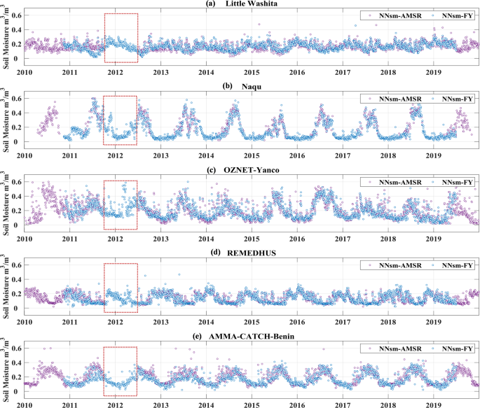
time series comparison of the NNsm-AMSR (purple dots) and NNsm-FY (blue dots) for period 2010 to 2019 over in situ networks: (a) Little Washita, (b) Naqu, (c) Yanco, (d) REMEDHUS, (e) Benin.
-
(2)
Homogeneity of NNsm_FY and NNsm_AMSR

Before combination usage of NNsm_FY and NNsm_AMSR, we evaluated the homogeneity of those two datasets. As shown in Fig. 11, NNsm_FY and NNsm_AMSR have the similar dynamic range and values of soil moisture. We also tested the consistency in terms of CC, bias Cumulative Distribution Function (CDF), and Quantile-Quantile plot(Q-Q plot), shown in the Fig. 12 (all global grid cells) and Table 6 (taking the grid cells where validation networks located as examples). The Q-Q plot and CDF, based on all of the daily data for the NNsm_FY and NNsm_AMSR in Fig. 12c,d, demonstrates that those two datasets have similar spatio-temporal distribution pattern. NNsm_FY agrees well with NNsm_AMSR, with high CC values in regions with significant soil moisture dynamics, and with most absolute values of bias less than 0.01 m3/m3, as shown in the Fig. 12a,b and Table 6.

Statistical comparisons of NNsm-FY with NNsm-AMSR in the whole FY-3B period (2010–2019) at each grid cell globally: (a) CC, (b) Bias(m3/m3), (c)CDF and (d) Q-Q plot.
Advantages of NNsm-FY
As described in the previous section, NNsm-FY has high accuracy, showing good agreement with SMAPsm and in situ observations, and performs better than FY-3B official soil moisture product (FY-sm) when comparing with in situ soil moisture. Filling in gap of NNsm-AMSR (2011.11–2012.06), NNsm-FY works together with NNsm-AMSR to provide complete long-term soil moisture since 2002, both having a high accuracy similar with SMAPsm.
For the convenience of application, we also compare data spatial coverage, taking 2018 as an example. In Fig. 13a, NNsm-FY can provide considerable amount of soil moisture retrievals at each grid cell globally. Another important detail worth mentioning is that, NNsm-FY has more soil moisture retrievals in the Tibetan Plateau and in some part of the high latitudes. FY-sm shown in Fig. 13b has no retrievals at most grid cell in the Tibetan Plateau, and has less retrievals in the high latitudes, caused by the failure of algorithm or flagging of frozen soil. In addition to high accuracy, our product NNsm-FY has a greater spatial coverage than SMAPsm and SMOSsm, especially in the Tibetan Plateau area, as shown in Fig. 13a,c,d. This is primarily determined by the satellite configuration, as swath width of SMAP and SMOS is 1000 km and swath width of FY-3 MWRI is 1400 km. In the Tibetan Plateau area, NNsm-FY has more retrievals both for swath width and retrieval algorithm. NNsm-AMSR in Fig. 13e can provide most soil moisture retrievals globally among those 5 single satellite products, except that NNsm-FY has more retrievals than NNsm-AMSR in the Tibetan Plateau. In Fig. 13f for CCIsm(Version v05.2), numbers of retrievals per year at some medium- and low-latitude grid cells are close to or equal to 365, namely CCIsm has retrievals almost every day at those gird cells, which is because CCIsm merged ASCAT, AMSR2, SMOS and SMAP into one product57. Even so, CCIsm has less retrievals in the Tibetan Plateau (less than 100 retrievals per year at one grid cell), due to the LPRM retrieval algorithm as well as different quality and uncertainties of other used soil moisture products.

Amount of soil moisture retrievals at each grid cell within 2018 for the following products: (a) NNsm-FY, (b) FY-sm, (c) SMAPsm, (d) SMOSsm, (e) NNsm-AMSR, and (f) CCIsm.
Code availability
The input data processing, dataset generation and validation were conducted using Matlab software (R2018b version). Code is available on Github: https://github.com/panpanyao/NNsm-FY-code.
References
Porporato, A., D’Odorico, P., Laio, F. & Rodriguez-Iturbe, I. Hydrologic controls on soil carbon and nitrogen cycles. I. Modeling scheme. Adv. Water Resour. 26, 45–58 (2003).
Falloon, P., Jones, C. D., Ades, M. & Paul, K. Direct soil moisture controls of future global soil carbon changes: An important source of uncertainty. Global Biogeochem. Cycles 25, 1–14 (2011).
McColl, K. A. et al. The global distribution and dynamics of surface soil moisture. Nat. Geosci. 10, 100–104 (2017).
Montzka, E. C. et al. Soil Moisture Product Validation Good Practices Protocol. https://doi.org/10.5067/doc/ceoswgcv/lpv/sm.001 (2020).
Oki, T. & Kanae, S. Global hydrological cycles and world water resources. Science (80-.). 313, 1068–1072 (2006).
Seneviratne, S. I. et al. Investigating soil moisture-climate interactions in a changing climate: A review. Earth-Science Rev. 99, 125–161 (2010).
Short Gianotti, D. J., Akbar, R., Feldman, A. F., Salvucci, G. D. & Entekhabi, D. Terrestrial Evaporation and Moisture Drainage in a Warmer Climate. Geophys. Res. Lett. 47, 1–12 (2020).
Short Gianotti, D. J., Rigden, A. J., Salvucci, G. D. & Entekhabi, D. Satellite and Station Observations Demonstrate Water Availability’s Effect on Continental-Scale Evaporative and Photosynthetic Land Surface Dynamics. Water Resour. Res. 55, 540–554 (2019).
Zhao, T. et al. Soil moisture experiment in the Luan River supporting new satellite mission opportunities. Remote Sens. Environ. 240 (2020).
Sheffield, J. & Wood, E. F. Global trends and variability in soil moisture and drought characteristics, 1950–2000, from observation-driven simulations of the terrestrial hydrologic cycle. J. Clim. 21, 432–458 (2008).
Ray, R. L., Jacobs, J. M. & Cosh, M. H. Landslide susceptibility mapping using downscaled AMSR-E soil moisture: A case study from Cleveland Corral, California, US. Remote Sens. Environ. 114, 2624–2636 (2010).
Lakshmi, V., Piechota, T., Narayan, U. & Tang, C. Soil moisture as an indicator of weather extremes. Geophys. Res. Lett. 31, 2–5 (2004).
Alexander, L. Climate science: Extreme heat rooted in dry soils. Nat. Geosci. 4, 12–13 (2011).
Fischer, E. M., Seneviratne, S. I., Vidale, P. L., Lüthi, D. & Schär, C. Soil moisture-atmosphere interactions during the 2003 European summer heat wave. J. Clim. 20, 5081–5099 (2007).
Hirschi, M., Mueller, B., Dorigo, W. & Seneviratne, S. I. Using remotely sensed soil moisture for land-atmosphere coupling diagnostics: The role of surface vs. root-zone soil moisture variability. Remote Sens. Environ. 154, 246–252 (2014).
Chen, F., Crow, W. T., Starks, P. J. & Moriasi, D. N. Improving hydrologic predictions of a catchment model via assimilation of surface soil moisture. Adv. Water Resour. 34, 526–536 (2011).
Scipal, K., Drusch, M. & Wagner, W. Assimilation of a ERS scatterometer derived soil moisture index in the ECMWF numerical weather prediction system. Adv. Water Resour. 31, 1101–1112 (2008).
Narasimhan, B., Srinivasan, R. & Arnold, J. G. & Di Luzio, M. Estimation of long-term soil moisture using a distributed parameter hydrologic model and verification using remotely sensed data. Trans. Am. Soc. Agric. Eng. 48, 1101–1113 (2005).
Huntington, T. G. Evidence for intensification of the global water cycle: Review and synthesis. J. Hydrol. 319, 83–95 (2006).
Jackson, T. J. III. Measuring surface soil moisture using passive microwave remote sensing. Hydrol. Process. 7, 139–152 (1993).
Koike, T. Description of GCOM-W1 AMSR2 Soil Moisture Algorithm. Descr. GCOM-W1 AMSR2 Lev. 1R Lev. 2 Algorithms 8.1–8.13 (2013).
Kerr, Y. H. et al. Soil moisture retrieval from space: The Soil Moisture and Ocean Salinity (SMOS) mission. IEEE Trans. Geosci. Remote Sens. 39, 1729–1735 (2001).
Entekhabi, D. et al. The soil moisture active passive (SMAP) mission. Proc. IEEE 98, 704–716 (2010).
Al-Yaari, A. et al. Testing regression equations to derive long-term global soil moisture datasets from passive microwave observations. Remote Sens. Environ. 180, 453–464 (2016).
Rodriguez-Fernandez, N. et al. Soil moisture retrieval from SMOS observations using neural networks. Int. Geosci. Remote Sens. Symp. 2431–2434, https://doi.org/10.1109/IGARSS.2014.6946963 (2014).
Rodríguez-Fernández, N. J. et al. Long term global surface soil moisture fields using an SMOS-Trained neural network applied to AMSR-E data. Remote Sens. 8 (2016).
Zhao, T. et al. Retrievals of soil moisture and vegetation optical depth using a multi-channel collaborative algorithm. Remote Sens. Environ. 257, 112321 (2021).
Owe, M., de Jeu, R. & Holmes, T. Multisensor historical climatology of satellite-derived global land surface moisture. J. Geophys. Res. Earth Surf. 113, F01002 (2008).
Liu, Y. Y. et al. Developing an improved soil moisture dataset by blending passive and active microwave satellite-based retrievals. Hydrol. Earth Syst. Sci. 15, 425–436 (2011).
Liu, Y. Y. et al. Trend-preserving blending of passive and active microwave soil moisture retrievals. Remote Sens. Environ. 123, 280–297 (2012).
Gruber, A., Dorigo, W. A., Crow, W. & Wagner, W. Triple Collocation-Based Merging of Satellite Soil Moisture Retrievals. IEEE Trans. Geosci. Remote Sens. 55, 6780–6792 (2017).
Liu, J. et al. Noaa soil moisture operational product system (smops) and its validations 1. Earth System Science Interdisciplinary Center (ESSIC)/Cooperative Institute for Climate & Satellite-Maryland (CICS-MD), University of Maryland, College Park, Maryland. 3477–3480 (2016).
Dorigo, W. et al. ESA CCI Soil Moisture for improved Earth system understanding: State-of-the art and future directions. Remote Sens. Environ. 203, 185–215 (2017).
Gruber, A., Scanlon, T., Van Der Schalie, R., Wagner, W. & Dorigo, W. Evolution of the ESA CCI Soil Moisture climate data records and their underlying merging methodology. Earth Syst. Sci. Data 11, 717–739 (2019).
Hollmann, R. et al. The ESA climate change initiative: Satellite data records for essential climate variables. Bull. Am. Meteorol. Soc. 94, 1541–1552 (2013).
Dorigo, W. A. et al. Evaluation of the ESA CCI soil moisture product using ground-based observations. Remote Sens. Environ. 162, 380–395 (2015).
Yao, P., Shi, J., Zhao, T., Lu, H. & Al-Yaari, A. Rebuilding long time series global soil moisture products using the neural network adopting the microwave vegetation index. Remote Sens. 9, 1–27 (2017).
Yao, P. & Lu, H. A long term global daily soil moisture dataset derived from AMSR-E and AMSR2 (2002-2022). Natinal Tibetan Plateau Data Center. https://doi.org/10.11888/Soil.tpdc.270960 (2020).
Yao, P. et al. A long term global daily soil moisture dataset derived from AMSR-E and AMSR2 (2002–2019). Sci. Data 8, 1–16 (2021).
Shi, J. et al. Microwave vegetation indices for short vegetation covers from satellite passive microwave sensor AMSR-E. Remote Sens. Environ. 112, 4285–4300 (2008).
Yao, P., Lu, H., Zhao, T., Wu, S. & Shi, J. A global daily soil moisture dataset derived from Chinese FengYun-3B Microwave Radiation Imager (MWRI) (2010–2019). National Tibetan Plateau Data Center. https://doi.org/10.11888/Terre.tpdc.271954 (2021).
Jackson, T. J. et al. Validation of advanced microwave scanning radiometer soil moisture products. IEEE Trans. Geosci. Remote Sens. 48, 4256–4272 (2010).
Cosh, M. H., Jackson, T. J., Starks, P. & Heathman, G. Temporal stability of surface soil moisture in the Little Washita River watershed and its applications in satellite soil moisture product validation. J. Hydrol. 323, 168–177 (2006).
Smith, A. B. et al. The Murrumbidgee Soil Moisture Monitoring Network data set. Water Resour. Res. 48, 1–6 (2012).
Pellarin, T. et al. Hydrological modelling and associated microwave emission of a semi-arid region in South-western Niger. J. Hydrol. 375, 262–272 (2009).
Dorigo, W. A. et al. The International Soil Moisture Network: A data hosting facility for global in situ soil moisture measurements. Hydrol. Earth Syst. Sci. 15, 1675–1698 (2011).
Dorigo, W. A. et al. Global Automated Quality Control of In Situ Soil Moisture Data from the International Soil Moisture Network. Vadose Zo. J. 12, vzj2012.0097 (2013).
Pastorello, G. et al. The FLUXNET2015 dataset and the ONEFlux processing pipeline for eddy covariance data. Sci. data 7, 225 (2020).
Warm Winter 2020 Team, & I. E. T. C. Warm Winter 2020 ecosystem eddy covariance flux product for 73 stations in FLUXNET-Archive format—release 2022-1 (Version 1.0). https://doi.org/10.18160/2G60-ZHAK (2022).
ICOS RI. Ecosystem final quality (L2) product in ETC-Archive format - release 2021-1. ICOS ERIC-Carbon Portal. https://doi.org/10.18160/FZMY-PG92 (2022).
Zhao, T. et al. Soil moisture retrievals using L-band radiometry from variable angular ground-based and airborne observations. Remote Sens. Environ. 248, 111958 (2020).
Calvet, J. C. et al. Sensitivity of passive microwave observations to soil moisture and vegetation water content: L-band to W-band. IEEE Trans. Geosci. Remote Sens. 49, 1190–1199 (2011).
Shi, J. et al. Physically based estimation of bare-surface soil moisture with the passive radiometers. IEEE Trans. Geosci. Remote Sens. 44, 3145–3152 (2006).
Sun, R., Zhang, Y., Wu, S., Yang, H. & Du, J. The FY-3B/MWRI soil moisture product and its application in drought monitoring. in International Geoscience and Remote Sensing Symposium (IGARSS) 3296–3298, https://doi.org/10.1109/IGARSS.2014.6947184 (2014).
Wang, H., Zan, B., Wei, J., Song, Y. & Mao, Q. Spatiotemporal Characteristics of Soil Moisture and Land–Atmosphere Coupling over the Tibetan Plateau Derived from Three Gridded Datasets. Remote Sens. 14, 5819 (2022).
Zhang, R. et al. Assessment of Agricultural Drought Using Soil Water Deficit Index Based on ERA5-Land Soil Moisture Data in Four Southern Provinces of China. Agriculture 11, 411 (2021).
Scanlon, T. et al. ESA Climate Change Initiative Plus - Soil Moisture Algorithm Theoretical Baseline Document (ATBD) D2.1 Version 04.7. ESA Bull. Version4.7, 73 (2020).
Peel, M. C., Finlayson, B. L. & McMahon, T. A. Updated world map of the Köppen-Geiger climate classification. Hydrol. Earth Syst. Sci. 11, 1633–1644 (2007).
Acknowledgements
This work was jointly supported by the National Natural Science Foundation of China (NSFC) (Grant no. 42090014), the Open Fund of Ministry of Education Key Laboratory for Earth System Modeling(Tsinghua University), the Second Tibetan Plateau Scientific Expedition and Research Program (2019QZKK0206), the National Key Research and Development Program of China (No. 2018YFB0504905). The authors thank NASA, NSIDC and NSMC for providing TB and SM products of SMAP and FY-3B. We acknowledge ISMN for providing in situ SSM observations. USDA is an equal opportunity provider and employer. This research was a contribution from the Long-Term Agroecosystem Research (LTAR) network. LTAR is supported by the United States Department of Agriculture. We acknowledge all the FLUXNET2015 sites, ICOS2020 sites, ICOSETC2022 site, AmeriFlux sites, TERN sites for their data records. Funding for AmeriFlux data resources was provided by the U.S. Department of Energy’s Office of Science. TERN flux data was sourced from Terrestrial Ecosystem Research Network (TERN) infrastructure, which is enabled by the Australian Government’s National Collaborative Research Infrastructure Strategy (NCRIS).
Author information
Authors and Affiliations
Contributions
P.Y., H.L. and P.Z. conceived this research; P.Y. performed the experiments and data processing, wrote the manuscript. H.L. and T.Z. gave detailed advice in the experiment and the manuscript writing, S.W. provided the re-calibrated FY-3B MWRI TB data and gave advices in data processing. J.S., K.Y., L.J., Z.P. and M.C. provided guidance and advice throughout the experiment and analysis and commented on the manuscript. K.Y. provided the Tibetan Plateau networks observations. M.C. provided the USDA networks observations and the validation suggestion.
Corresponding authors
Ethics declarations
Competing interests
The authors declare no competing interests.
Additional information
Publisher’s note Springer Nature remains neutral with regard to jurisdictional claims in published maps and institutional affiliations.
Rights and permissions
Open Access This article is licensed under a Creative Commons Attribution 4.0 International License, which permits use, sharing, adaptation, distribution and reproduction in any medium or format, as long as you give appropriate credit to the original author(s) and the source, provide a link to the Creative Commons license, and indicate if changes were made. The images or other third party material in this article are included in the article’s Creative Commons license, unless indicated otherwise in a credit line to the material. If material is not included in the article’s Creative Commons license and your intended use is not permitted by statutory regulation or exceeds the permitted use, you will need to obtain permission directly from the copyright holder. To view a copy of this license, visit http://creativecommons.org/licenses/by/4.0/.
About this article

Cite this article
Yao, P., Lu, H., Zhao, T. et al. A global daily soil moisture dataset derived from Chinese FengYun Microwave Radiation Imager (MWRI)(2010–2019). Sci Data 10, 133 (2023). https://doi.org/10.1038/s41597-023-02007-3
Received:
Accepted:
Published:
DOI: https://doi.org/10.1038/s41597-023-02007-3
