
Abstract
Single-virus tracking (SVT) offers the opportunity to monitor the journey of individual viruses in real time and to explore the interactions between viral and cellular structures in live cells, which can assist in characterizing the complex infection process and revealing the associated dynamic mechanisms. However, the low brightness and poor photostability of conventional fluorescent tags (e.g., organic dyes and fluorescent proteins) greatly limit the development of the SVT technique, and challenges remain in performing multicolor SVT over long periods of time. Owing to the outstanding photostability, high brightness and narrow emission with tunable color range of quantum dots (QDs), QD-based SVT (QSVT) enables us to follow the fate of individual viruses interacting with different cellular structures at the single-virus level for milliseconds to hours, providing more accurate and detailed information regarding viral infection in live cells. So far, the QSVT technique has yielded spectacular achievements in uncovering the mechanisms associated with virus entry, trafficking and egress. Here, we provide a detailed protocol for QSVT implementation using the viruses that we have previously studied systematically as an example. The specific procedures for performing QSVT experiments in live cells are described, including virus preparation, the QD labeling strategies, imaging approaches, image processing and data analysis. The protocol takes 1–2 weeks from the preparation of viruses and cellular specimens to image acquisition, and 1 d for image processing and data analysis.
Introduction
Viruses are strictly intracellular parasites that accomplish their own life activities by hijacking the metabolism of the host cell. Viral infection begins with the binding of a virus to a specific receptor on the cell surface. Then some viruses fuse with the plasma membrane by interacting with membrane receptors and the lipid microenvironment to release their genome into the host cell. Other viruses enter the host cell via endocytosis and are then sequestered in specific organelles, releasing their genomes to targeted sites for replication under the appropriate conditions. After being accumulated for a period of time, the newly synthesized viral proteins and viral genome are packaged into infectious progeny that exit the cell via cell lysis and exocytosis1,2. Thus, the viral journey in the host cell is a complex and dynamic process involving multiple infection pathways and steps, dissociation of viral components and complex interactions with cellular structures3,4. Therefore, the comprehensive understanding of the dynamics and mechanisms involved in viral infection may contribute to the prevention and treatment of viral diseases and the development of antiviral drugs.
The quantum dot (QD)-based single-virus tracking (QSVT) technique is an imaging approach that uses QDs as fluorescent tags to label different viral components and fluorescence microscopy to investigate the infection process of single viruses and the dynamic relationship between viruses and cellular components5,6. In QSVT experiments, the behavior of a single virus or viral component labeled with QDs can be monitored within a host cell for long term and in real time. After reconstructing the movement trajectories of individual viruses, the associated dynamic information can be extracted meticulously to reveal the infection mechanism of viruses. The extremely high brightness and excellent photostability of QDs facilitate high-contrast and long-time span imaging of individual viruses from milliseconds to hours, and allow for the localization of individual viruses with nanometer-level precision7. The color-tunable emission with a narrow full width at half maximum makes QDs an excellent label for synchronous multicomponent labeling of viruses, with single-virus sensitivity8. Therefore, QDs have greatly facilitated the development of the single-virus tracking (SVT) technique, especially for applications such as viral journeys requiring long-term and multicolor imaging, and single-virus level studies of virus–cell interactions9,10,11,12,13,14.
Development of the protocol
The concept of SVT emerged in the early twenty-first century, when organic dyes, as a conventional fluorescent tag easily available from commercial companies, were used to label different viral components to enable the tracking of individual viruses in live cells15,16,17. Notably, benefiting from lipophilic dye labeling, changes in fluorescence intensity of individual viruses have been widely used to detect the virus–endosome fusion events for genome release in live cells16,18,19. Fluorescent proteins (FPs), with colors covering almost the entire visible region and even the near-infrared light region, can be genetically manipulated to achieve site-specific protein labeling in live cells and are commonly used to label viral components and cellular structures20,21,22,23,24,25. However, some inherent limitations of organic dyes and FPs, such as comparatively low fluorescence signal, inferior photostability and wide absorption/emission spectra, lead to harsh imaging conditions, cumbersome experimental operations and poor experimental reproducibility8, which greatly limit the application of the SVT technique for long-term, multicolor tracking of viral components during the infection process.
Fluorescent semiconductor QDs, as inorganic nanocrystals composed of II–VI, III–V and IV–VI periodic elements, have attracted wide interest from researchers owing to their special photophysical properties such as superior brightness, high photostability, broad absorption, narrow and size-tunable fluorescent emission, and large Stokes shift26. They have been used in many applications such as biomarkers, biosensing and bioimaging7,26,27,28,29. Advances in QD synthesis and biofunctionalization techniques have made them appealing as fluorophores for labeling different components of viruses6,12,14,30,31,32,33,34, which in turn has facilitated the development of the long-term, multicolor QSVT technique14,35,36,37,38, enabling the visualization of dynamic molecular events during viral infection that were difficult to observe with prior approaches.
We have been conducting researches related to QSVT for the past decade, and have done a lot of work to promote the development of this technique and to systematically explore the mechanisms of virus infection9,35,36,39,40,41,42,43. In particular, many methodological improvements in the QSVT technique have been made in recent years, not only in the strategies of virus labeling with QDs44,45,46,47, but more importantly in the image processing and imaging algorithms10,11,48,49, making the QSVT technique a mature and commonly used method for virus tracking. Here, we present a protocol to illustrate how QSVT can be readily used to decipher complex infection processes of viruses and uncover the underlying mechanisms. We have refined and standardized the steps of QSVT in this protocol, which has and will continue to allow researchers to better use this remarkable tool in virological research.
Overview of the procedure
The key steps in performing QSVT experiments include the following six stages (Fig. 1):

To obtain labeled virus samples for imaging, protocols for the propagation, purification and characterization of virus depend strongly on the virus type (stage 1). Next, cell structure labeling and drug inhibition assays can be used to facilitate the exploration of the dynamic interactions between virus and cellular structures and the steps of the infection process (stage 2). Labeling viral components with QDs is crucial for QSVT. The appropriate labeling method needs to be carefully chosen to avoid affecting the viral infectivity. The labeled viruses are then incubated with host cells for imaging (stage 3). Then, labeled viruses can be individually tracked with two-dimensional, three-dimensional or multicolor QSVT techniques using a SDCM to obtain time-series images (stage 4). After that, image processing is required to convert the original stack of fluorescent images into trajectories (stage 5). Finally, on the basis of the time-dependent plot of speed or intensity, MSD and colocalization, the trajectories are statistically analyzed to uncover the underlying mechanisms of virus infection (stage 6).
Stage 1: virus amplification and characterization. Virus stocks should first be amplified and purified to obtain samples that meet the requirements for efficient labeling of viruses to avoid interference of nonviral structures during imaging.
Stage 2: cell labeling and drug inhibition. Cells need to be seeded in a glass-bottomed Petri dish for confocal imaging. Since the dynamic interactions between cellular and viral components is a continuous process throughout the entire life cycle of a virus, labeling of cellular structures with FPs or organic dyes can be used to identify the specific locations of viruses in live cells, and inhibition of cellular function with common inhibitors can be used to identify cellular uptake and transport pathways of viral infection. Thus, cell labeling and drug inhibition are optional steps to investigate the different phases of viral infection, which can be selected to treat cell samples separately or simultaneously before imaging, depending on the experimental purpose.
Stage 3: virus labeling with QDs. During the viral journey to infect a live cell, different components of the virus are dynamically disassembled as the infection process advances, and therefore both inner and outer components of the virus should be labeled with QDs separately or simultaneously to comprehensively understand the mechanism of viral infection. Once the labeled viruses are incubated with the cells cultured in the Petri dish, the infection is initiated and imaging can be performed.
Stage 4: image acquisition. The infection behavior of individual viruses in live cells can be monitored with fluorescent microscopes equipped with detectors of sufficient sensitivity and fast acquisition capabilities. Two-dimensional (2D), three-dimensional (3D) and multicolor QSVT techniques can be performed by using a spinning-disk confocal microscope (SDCM) to accurately track the motility behavior of individual viral particles.
Stage 5: image processing. After the microscope images containing a large amount of information are acquired, the trajectories of the virus infection behaviors need to be obtained through image processing steps, including noise reduction, particle localization and trajectory reconstruction.
Stage 6: data analysis. Finally, the dynamic parameters associated with the viral infection are extracted by analyzing the viral motion trajectories, including transport characteristics analysis, fluorescence intensity analysis and multicolor image analysis, to reveal the underlying viral infection mechanism.
Applications of the protocol
Virus infection is a complex process in which viruses interact dynamically with host cells in a spatio–temporal manner (Fig. 2)1,4. The QSVT technique facilitates in-depth study of the transport behavior of various animal viruses in their host cells and potential mechanisms of infection pathways. By complementing with cell labeling techniques and drug inhibition assays, this technique allows extensive access to dynamic information about the cellular components associated with viruses to reveal their underlying biological mechanisms, examples of which are discussed in the following sections. Thus, the technique is suitable for a wide range of situations where the dynamic mechanisms of viral infection need to be studied. For example, the dynamic infection mechanisms of emerging viruses urgently require this technique, and the strategies and tools developed so far may advance the field of virus prophylaxis and virus vaccine development.

The process of virus infection in live cells involves virus entry, virus transport, virus assembly and virus budding. The virus first binds to the receptor after attaching to the cell membrane. Most viruses enter the cell via CME (1), caveolin-mediated endocytosis (2), or nonclathrin and noncaveolin endocytosis (3). The virus trapped in the endosome is then transported along actin filaments and microtubules to the microtubule organizing center (MTOC). After fusing with the appropriate endosome, viral genomes can be released into the cytosol or the nucleus. Some viruses can fuse with the plasma membrane directly, allowing for direct genome release into the cytosol (4). The newly synthesized viral genome is then packaged into the capsid and envelope near the MTOC and transported to the cell periphery via microtubules, after which the virus is released into the extracellular environment (i). Some capsids can also be encapsulated by the plasma membrane and released to the outside of the cell (ii).
Virus entry into host cells
An important issue in virus infection of host cells is how the virus internalizes into the cell by means of the host cell’s endocytic pathways. QSVT has greatly contributed to the study of the dynamic mechanisms of the viral internalization process36,48. For example, QSVT showed that influenza A viruses (IAVs) tend to bind to sialic acid receptors on the cell surface and then enter the host cell via the endocytic pathway. Further systematic studies revealed two distinct pathways of internalization for IAVs. When IAVs attached to the receptors on the cell surface, most of them were internalized by forming clathrin-coated vesicles with the help of dynamin. Other viruses entered the cell in a clathrin-independent manner, relying only on dynamin41.
Virus transport along cytoskeleton
Viruses that enter cells by endocytosis are encapsulated in endosomes and transported along the cytoskeleton towards the vicinity of the nucleus. By tracking the infection behavior of IAV over 30 min, we analyzed the population behavior of viruses within individual cells, revealing five stages of viral infection processes associated with early and late endosomes35. In addition, QSVT was used to investigate the effect of microtubule geometry on viral behaviors in live cells, and elucidated the ‘drive switch’ mechanism responsible for the seamless delivery of virus from myosin VI to microtubules by the molecular motor switch9,50. By performing long-term and multicolor real-time QSVT, we also found that ~20% of the virus internalized by the cell was trapped in autophagosomes lacking Rab5, which subsequently moved from the cell periphery to the perinuclear region via microtubules for infection43. Meanwhile, since Rab5 and Rab7 are proteins responsible for the regulation of endosome transport and maturation, we explored the Rab5- and Rab7-related infection behavior of IAVs using the 3D QSVT technique, and revealed the different dynamic behavior of Rab5- and Rab7-positive endosomes involved in the intracellular transport of viruses51.
Virus uncoating during infection
Once the virus reaches the inner region of the cell, it releases the genome from its dense package into the cytoplasm or nucleus for subsequent replication. Most of the enveloped viruses release their genomes by fusion of the viral envelope and the endosomal membrane at low pH11. By wrapping QD-bound viral ribonucleoprotein complexes in infectious IAV virions, QSVT revealed that ~30% of IAV viral particles trigger uncoating by fusion with late endosomes in the perinuclear region within 30–90 min after infection37. By combining QSVT with in situ quantification of pH, we have achieved real-time visualization and quantification of the genome release process at the single-virus level, revealing that Japanese encephalitis virus (JEV) genome release events occur primarily in the mature endosome, an intermediate stage between the early and late endosomes, resolving the long-standing question of where JEV releases its genome for replication10.
Comparison with other methods
Compared with strategies using organic dyes and FPs as tags for SVT, QSVT has notable advantages in the following aspects: (i) the brilliant brightness of QDs makes it possible to use very few or even only one QD to achieve viral labeling that facilitates SVT; (ii) the excellent photostability of QDs allows them to be used to track the infection process of individual viruses over a long period; (iii) the color-tunable emission characteristics make it possible to simultaneously label various components of the virus with multiple colors and (iv) the abundance of surface ligands on QDs facilitates the labeling of different components of the virus by various labeling strategies5. By further combining QD labeling strategies with 3D QSVT, several researchers have successfully revealed new dynamic mechanisms of virus infection48,49,51. Organic dyes and FPs do have a natural advantage in labeling the cytoskeleton as well as the internal components of the virus, and can be used as an aid for short time tracking of viral components or precise localization of the virus within the host cell. Therefore, we emphasize that the combined use of these fluorescent labels for SVT techniques is essential.
Limitations of QSVT
The process of viral infection involves interactions between viral and cellular components, so to obtain more accurate information by QSVT, not only high-performance QDs are required, but also site-specific, quantitative in-situ labeling methods designed according to the characteristics of the viral structure and dynamic infection process are crucial to reducing interference with the viral infection behavior. Although the brilliant brightness of QDs facilitates high signal-to-noise (S/N) single-QD tracking to explore how molecules move dynamically and in a coordinated manner in the cell to ensure cell structure and function, labeling viral components with only one QD remains a great challenge in implementation. Although genetically engineered site-specific labeling methods can enable the labeling of a protein with a single QD, it remains a challenge to label a viral particle with a single QD because viruses have complex structures that often contain multiple identical proteins.
So far, monitoring the dynamic process of virus assembly and egress with QSVT remains a major challenge as nascent progeny viruses and their components are difficult to label with QDs efficiently. With the further development of QD labeling strategies and the combination with other novel technologies, the QSVT technique holds the promise of becoming a powerful tool to probe the entire dynamic process of virus infection. Furthermore, the majority of current QSVT studies have been conducted at the cellular level, which does not provide the most realistic and valuable dynamic information in revealing the infection mechanisms of viruses in vivo. As a result, there is an urgent need to work on new labeling and imaging strategies to monitor the infection behaviors of viruses in living tissues or in vivo.
Expertise and equipment needed to implement the protocol
The implementation of this technique requires the use of well-equipped microscopy instruments and a high biosafety level laboratory (≥P2 level). The protocol will be easier to perform if the operator is skilled in nanoparticle biofunctionalization, cell and virus culture, and microscope operation.
Experimental design
Stage 1: virus amplification and purification (Steps 1–8)
Our laboratory has applied the QSVT technique mainly to four virus strains, namely IAV9,11,41,48, JEV10,52, pseudorabies virus40, and baculovirus44,46. In this protocol, we chose IAV and JEV as models to study the dynamic infection mechanisms of these two kinds of virus in their host cells (Madin–Darby canine kidney cell line (MDCK) cells for IAV and baby hamster kidney-21 (BHK-21) cells for JEV). To obtain efficiently labeled virus samples for imaging in the context of nonviral structures, it is often recommended to start with amplification and purification of the virus to obtain a concentrated virus stock solution. The procedures for growing, isolating and purifying viruses vary considerably depending on the type of virus. Virus stocks are usually generated by infecting cells in large-scale culture medium or allowing viruses to grow in eggs or live animals. Precipitation and concentration by ultracentrifugation with a density gradient are classic purification methods (e.g., sucrose and cesium chloride). In addition, some viruses are now available in purified form as commercial products from related biotechnology companies. In this section, we present the detailed steps of virus amplification and purification in embryonated eggs and live cells, using IAV and JEV as examples, respectively. Next, transmission electron microscopy and titer assays can be used to examine viral integrity and infectivity.
Stage 2: cell labeling and drug inhibition (Steps 9–11)
Confocal microscopy is an essential tool to investigate the infection behavior of individual viruses in live cells, which requires the cells to be cultured in a glass-bottomed Petri dish for imaging. Since the occurrence of virus–host interactions continues throughout the course of viral infection, the combination of QSVT techniques with cell structure labeling or drug inhibition assays is optional for the exploration of the dynamic interactions between virus and cellular structures and different stages of the entire infection process.
Labeling cellular proteins with FPs is frequently useful (Step 11A). This is accomplished by fusing the FP gene to the gene of interest and expressing the fusion protein in the host cell, either transiently or stably. Transient transfection is much faster and can be accomplished more easily, but can result in inconsistent levels of expression of FPs, and overexpression of FPs can be severely detrimental to cell health and proliferation. Therefore, when using FPs for QSVT experiments, the relevant functional validation experiments need to be performed to test for such adverse effects. It is optional to generate stable cell lines that exhibit the expression of transfected protein at consistent levels in each cell, but the procedure of stable transfection is cumbersome and time consuming. Following stable transfection, a population of cells with low but discernible expression levels can also be chosen to eliminate the influence of the overexpression of transfected proteins on cell function. Thus, optimal expression levels of the fusion protein are required to detect individual cellular structures without interfering with cellular processes.
Small-molecule inhibitors can be used to identify cellular uptake and transport mechanisms (Step 11B). In this section, we used the example of drugs that depolymerize actin networks (cytochalasin D) and microtubules (nocodazole) to inhibit cytoskeleton-dependent transport. The required dose and exposure time of the drug should be verified by immunofluorescent staining for actin or tubulin to verify the disruption of the cytoskeletal network. Moreover, the drug should be kept in the imaging medium for the whole experiment to ensure that the cytoskeletal structure is disrupted continuously. The drug inhibition and cell labeling can be used to process the same cell samples simultaneously, depending on the experimental demand.
Stage 3: virus labeling with QDs (Step 12)
The next step to perform QSVT experiments is to use QDs to label the viral components. For the outer components of viruses, the QD labeling strategies we have developed for QSVT are mainly based on biotin–streptavidin interaction47,52 and direct chemical coupling45. In Step 12 we describe four options: option A for labeling viral outer components with QDs on the basis of biotin–streptavidin interaction; option B for labeling viral outer components with QDs on the basis of direct chemical coupling; option C for dual labeling of viral inner and outer components with QDs on the basis of electroporation or option D for dual labeling of viral inner with organic dyes and outer components with QDs on the basis of capsid breathing motion (a dynamic process of conformational change of the viral capsid). These labeling methods shed light on the mechanisms of viral entry and transport. However, they cannot be used to detect the separation of the viral genome from the external components of the virus, resulting in the loss of critical information about the genome release event following membrane fusion. Therefore, to comprehensively understand the mechanism of viral infection, it is crucial to effectively label and track the different viral components, especially the viral genome, during viral infection. Unfortunately, once the genome is assembled into the virus, it is difficult to attach external labels. To help labels break through the external barrier of the virus and label inner components, we developed two labeling strategies based on electroporation and capsid breathing motion10,53.
Biotin–streptavidin labeling strategies use biotinylated reagents, such as sulfosuccinimidyl-6-(biotin-amino)hexanoate (Sulfo-NHS-LC-biotin) or DSPE-PEG2000-biotin, to modify the viral surface with biotin and then streptavidin-modified QDs (SA-QDs) can bind to it via the biotin–streptavidin interaction. Sulfo-NHS-LC-biotin and DSPE-PEG2000-biotin achieve biotin modification of viruses by covalent coupling to amino groups on the virus surface and hydrophobic interactions inserted into the viral envelope, respectively. Therefore, Sulfo-NHS-LC-biotin is suitable for both enveloped and nonenveloped viruses, but DSPE-PEG2000-biotin is only suitable for enveloped viruses with a lipid layer.
The direct chemical coupling strategy utilizes 4-formylbenzoate (4FB)-modified QDs (4FB-QDs) to directly label 6-hydrazinylacetone hydrazone (HyNic)-modified viruses by covalent bonding; 4FB-QDs can be obtained by the reaction between amino-modified quantum dots (NH2-QDs) and succinimidyl 4-formylbenzoate (NHS-4FB) (Step 12B(i)). Optionally, the successful preparation of 4FB-QDs could be characterized by the slower migration rate of 4FB-QDs than NH2-QDs by agarose gel electrophoresis. Also, 5 μL of the solutions containing 4FB-QDs and NH2-QDs could be dropped on a cover glass, respectively, and fluorescence images of 4FB-QDs and NH2-QDs can be acquired by confocal microscopy. The fluorescence intensity of the two samples can be analyzed and compared to ensure that individual 4FB-QDs still retained high fluorescence brightness for further use.
Dual labeling of viral inner and outer components using electroporation is achieved by using direct chemical coupling to label the viral outer components as in option B, and using an electroporator to deliver nucleoprotein antibody-modified QDs (NPAb-QDs) to label the viral inner components. Briefly, as viruses contain multiple proteins, QDs modified with primary antibodies to viral proteins can be used to label viral proteins through antigen–antibody interactions. Immunofluorescent labeling of viral proteins is achieved by first binding the primary antibody to the target viral protein through antigen–antibody interaction, and then labeling the primary antibody with a fluorescently labeled secondary antibody. For multicolor QSVT, QDs with different emission wavelengths that can be well separated by emission filters should be selected. As the emission bands of QDs are generally narrow, they can easily meet the needs of multicolor QSVT experiments. Besides, benefiting from the high brightness of QDs, the excitation intensity can be kept as low as possible to achieve the desired S/N ratio and frame interval while protecting the cells from photodamage.
Dual labeling of viral inner and outer components on the basis of capsid breathing motion uses the biotin–streptavidin interaction to achieve QDs labeling of the outer components of the virus as in option A, and multiple molecular beacons (MMB) labeling of the genome of the virus by capsid breathing. MMBs are designed to specifically bind the viral genome, recovering fluorescent signals after binding to enable labeling of viral nucleic acids10.
Labeling efficiency can be assessed by colocalization analysis of immunofluorescence of viral proteins or fluorescence of Syto 82 (nucleic acid dye)-labeled viral genomes with fluorescence of QDs, and further verified by comparing the differences in hydrodynamic size and zeta potential of labeled and wild-type viruses53. The titer of labeled viruses also needs to be tested to assess the influence of the labeling process on viral infectivity.
Stage 4: image acquisition (Step 13)
A typical QSVT device consists of an inverted microscope, several lasers, a high numerical aperture objective and a sensitive detector. In contrast to wide-field fluorescence microscopy, confocal microscopy can eliminate or reduce fluorescence beyond the focal plane, allowing for continuous optical sectioning of cells and 3D QSVT in live cells. Owing to its high power and narrow band beam, this laser has been utilized increasingly as a light source for QSVT devices to minimize background noise in images. To capture as many fluorescence signals as possible from the excitation, the confocal equipment is always fitted with a high numerical aperture for the objective and a sharp fluorescence filter with high transmittance (>80%). For real-time monitoring, the imaging instrument should also be equipped with a high-sensitivity and high-speed detector with fast frame transfer and high quantum yield to obtain a high S/N ratio image. Electron multiplying charge-coupled device detectors can have fast readout speeds, high quantum yields and optimal resolution. With the ability to simultaneously excite more points in the focal plane, the SDCM can be combined with an electron multiplying charge-coupled device to obtain high spatial and temporal resolution sequence images, which are well suited for QSVT experiments. Combined with the color-tunable emission wavelength and a narrow full width at half-maximum of QDs, multicolor QSVT experiments can be performed using this equipment. If dynamic data on different components of viruses and cells need to be collected simultaneously, these components can be labeled with QDs or other fluorescent labels with different emission wavelengths. Simultaneous multichannel QSVT requires excitation of different fluorescent tags with lasers of different wavelengths and separation of the emitted light with emission filters to enable acquisition of multicolor images. Owing to the limitations of current confocal microscopy instruments, only four-color imaging is usually possible at most.
Stage 5: image processing (Step 14)
After recording the images, there are several image processing steps used to precisely track single viruses in live cells, including minimizing image noise, identifying virus positions and reconstructing trajectories. First, to reduce the interference of background noise on the localization precision of viral particles, we use a spatial filter to reduce background noise. Owing to the diffraction limit, the optical microscope has a resolution of ~250 nm in the lateral direction and ~500 nm in the axial direction, so the center of the viral particles should be precisely detected by localization algorithms (e.g., centroid, Gaussian fitting and radial symmetry algorithm)49. Next, the trajectory of a particle can be reconstructed by connecting its specific position in each frame. Manual linking is a general method, but is time consuming and subjective because the eyes can recognize only apparent particle motions, such as movement or nonmovement. Automatic linking methods typically utilize the shape, size and intensity of particles to link their positions in each frame, which is a more robust approach for reconstructing the trajectories of viruses. Additionally, when images are captured using multiple-color channels, fluorescence signals of aligned color channels can be used to measure the colocalization of two different fluorescently labeled structures. Fluorescence intensity versus time curves can be calculated for each color channel associated with the tracking point, and the dynamic interactions between these labeled structures can be examined by comparing them with the local background levels of each channel.
Different data types can be analyzed using specific software to improve the efficiency of the analysis. Image-Pro Plus (IPP) is particularly suitable for the reconstruction of 2D trajectories and the extraction of parameters such as velocity, distance, fluorescence intensity, etc. It is notably intuitive and easy to use. Imaris is a microscopic image analysis software focused on 3D images, with a sharper field of view and faster processing when working with 3D QSVT data, making it well suited for batch extraction and analysis of 3D trajectories. ImageJ has some unique advantages when processing multicolor QSVT data for kymograph, colocalization and statistical analysis between different channels.
Stage 6: data analysis (Steps 15–27)
Viruses usually change their motion behavior during infection, for example, viruses cross the cell membrane in a restricted manner, transport in a directional manner in the cytoplasm and move around the nucleus in a bidirectional diffusion manner. With the help of an instantaneous velocity versus time plot, different motion patterns of the trajectory can be differentiated and analyzed separately. Analysis of the mean square displacement (MSD) of virus trajectory is also a desirable way to characterize the viral particle transport properties. By calculating the MSD as a function of time lag, the movement behaviors of viruses can be classified into normal diffusion (also known as Brownian motion), directional motion, confined/corralled diffusion and anomalous diffusion. Some analyses are performed directly, for example, to observe colocalization and interactions between diverse structures and viral components, or to quantify the kinetics of virus entry by increasing and saturating the fluorescence intensity. To obtain realistic and unbiased information about the viral motility and virus–cell interactions to better assess virus infection process, it is essential to acquire hundreds or even thousands of virus trajectories through multiple independent experiments for statistical analysis.
Controls
Negative and positive controls are always needed throughout the experiment. During the virus labeling stage, negative controls can be selected from either the virus-free treatment group or the target-loss treatment group (e.g., where incorrect targeting sequences are involved during capsid breathing). Positive controls can be selected from other known targeting dyes or antibodies for labeling of viral targets. The labeling efficiency of the experimental group can also be obtained by assessing the degree of colocalization of the experimental group with the positive control group. At this stage, we also recommend to evaluate the labeling efficiency for viruses either fixed on the slide or bound to the surface of cell membranes. When treating cells with inhibitors, the cells need to be immersed in medium containing the inhibitor at all times to prevent weakening or loss of the inhibitory effect. In addition to the negative control (no inhibitor group), as many inhibitors have been reported to cause damage to cell health and proliferation at high concentrations, we recommend performing an additional toxicity control at this stage for the dose of inhibitor used. Imaging parameters (e.g., exposure time, laser power, frame interval, etc.) need to be as consistent as possible, in addition to using unlabeled viruses as negative controls during imaging. When analyzing trajectories, we recommend batch analysis and statistics of trajectories to minimize subjective bias.
Materials
Biological materials
-
Cell lines of interest. MDCK (ATCC, cat. no. CCL 334; RRID: CVCL_0422) and BHK-21 cell line (ATCC, cat. no. CCL-10; RRID: CVCL_1914) were used in this protocol
Caution
Cell lines should be maintained at 37 °C in a 5% CO2 and humidified atmosphere and checked periodically to ensure their authenticity and protection from mycoplasma contamination.
-
Viruses of interest. We used IAV (H9N2; A/chicken/Hubei/01-MA01/1999) and live-attenuated JEV (SA-14-14-2; GenBank accession number: AF315119) with known titer from previous preparations (IAV and JEV were provided by Prof. Han-Zhong Wang and Prof. Gengfu Xiao of Wuhan Institute of Virology, Chinese Academy of Sciences, respectively)
Caution
All materials and experiments involving viruses should be conducted in a class II biosafety cabinet in approved biosafety level 2 or higher biosafety level laboratory with appropriate personal protective equipment. Some high pathogenic viruses require a higher biosafety level. Persons planning to conduct experiments with samples that are known or intended to contain viruses must confer with institutional committees and government agencies before beginning any work to ensure that all experiments comply with relevant biosafety regulations.
-
9–11-d-old specific-pathogen-free (SPF) embryonated chicken eggs (Boehringer Ingelheim Viton Biotechnology)
Caution
Experiments with live animals must conform to all relevant institutional regulations. All animal experiments were approved by the institutional animal care and use committee, Center for Animal Experiment of Wuhan University.
Reagents
General reagents
-
Ultrapure water (from Milli-Q direct water purification system)
-
Ethanol, 70% (vol/vol)
-
Sodium chloride (NaCl; Solarbio, cat. no. S8210)
-
Potassium chloride (KCl; Solarbio, cat. no. P9921)
-
Calcium chloride (CaCl2; Solarbio, cat. no. C7250)
Caution
High energy release when it dissolves in water.
-
Sodium bicarbonate (NaHCO3; Solarbio, cat. no. S5240)
-
Magnesium chloride (MgCl2; Sigma-Aldrich, cat. no. M8266)
-
Hydrochloric acid (HCl; Sigma-Aldrich, cat. no. 258148)
Caution
May cause serious burns. Avoid direct contact with skin and eyes. Use in a fume hood. Wear gloves and protective equipment.
-
Dimethyl sulfoxide (DMSO; Sigma-Aldrich, cat. no. D8418)
Caution
DMSO is hazardous and corrosive. Keep away from skin and eyes. Wear gloves and protective equipment.
-
HEPES (Sigma-Aldrich, cat. no. H3375)
-
Glucose (Sigma-Aldrich, cat. no. 49163)
-
Phosphate buffered saline (PBS), pH 7.4 (Life Technologies, cat. no.10010-023)
-
Triton X-100 (Aladdin, cat. no. T109026-1L)
-
Phosphotungstic acid hydrate (Sango Biotech, cat. no. A601241)
Virus amplification and purification
-
Paraffin wax (Sigma-Aldrich, cat. no. 411663)
-
Sodium citrate buffer (Solarbio, cat. no. C1010)
-
N-tosyl-l-phenylalanine chloromethyl ketone–trypsin (Aladdin, cat. no. T128771-100 mg)
-
Chicken red blood cells (RBCs), 5% (vol/vol) (Lampire, cat. no. 7241409)
-
Methylcellulose (Sango Biotech, cat. no. A600616)
-
Crystal violet (Sango Biotech, cat. no. A600331)
-
Bradford protein assay kit (Solarbio, cat. no. PC0010)
Cell culture
-
Trypsin–EDTA, phenol red (Thermo Fisher Scientific, cat. no. 25300-62)
-
Dulbecco’s modified Eagle medium (DMEM) (Sigma-Aldrich, cat. no. D0819)
Critical
Comply with the manufacturer’s recommended storage conditions and shelf life.
-
Fetal bovine serum (FBS; Sigma-Aldrich, cat. no. 12003C)
-
Penicillin–streptomycin–glutamine solution 100× solution (Thermo Fisher Scientific, cat. no. 10378-016)
Virus labeling
-
DSPE-PEG2000-biotin (Avanti, cat. no. 880129P-10 mg)
-
Sulfo-NHS-LC-biotin (Thermo Fisher Scientific, cat. no. 21335)
-
605 nm-, 625 nm- and 705 nm-emitting SA-QDs (Wuhan Jiayuan)
-
525 nm- and 605 nm-emitting NH2-QDs, (Wuhan Jiayuan,)
-
NHS-4FB (Yuanye, cat. no. Y39997)
-
Succinimidyl 6-hydrazinonicotinate acetone hydrazone (NHS-HyNic; Heliosense, cat. no. HS-12008025)
-
Dithiothreitol (DTT; Thermo Fisher Scientific, cat. no. R0861)
Caution
DTT is toxic by aspiration and harmful in contact with skin or mucosa. Wear gloves and protective equipment.
-
4-(N-maleimidomethyl) cyclohexane-1-carboxylic acid 3-sulfo-N-hydroxysuccinimide ester sodium salt (Sulfo-SMCC; Thermo Fisher Scientific, cat. no. 22322)
-
NPAb (Abcam, cat. no. ab128193)
-
MMBs (Sango Biotech) (the MMB sequences used in this protocol are included in ref. 10)
Cell labeling and drug inhibition
-
Syto82 (Thermo Fisher Scientific, cat. no. S11363)
Critical
For best labeling effects, dissolve in DMSO and store at −20 °C away from light.
-
Lipofectamine LTX reagent (Thermo Fisher Scientific, cat. no.15338500)
-
Opti-MEM I medium (Thermo Fisher Scientific, cat. no.11058021)
-
Nocodazole (Sigma-Aldrich, cat. no. 487928)
-
Cytochalasin-D (Cyto-D; Sigma-Aldrich, cat. no. C2618)
-
d-Glucose (Solarbio, cat. no. G8150)
-
GFP1-clathrin light chain (Clc) plasmid (available from authors upon request)
-
Sodium azide (Sigma-Aldrich, cat. no. S2002)
Caution
Sodium azide is highly toxic by aspiration and harmful in contact with skin or mucosa. Wear gloves and protective equipment.
Agarose gel electrophoresis
-
Tris–acetate–EDTA (TAE), 10× (Invitrogen, cat. no. 15558042)
-
Agarose RA, biotechnology grade (VWR Life Science, cat. no. 97064-258)
Immunofluorescence
-
Paraformaldehyde (Sango Biotech, cat. no. A500684)
-
Anti-Japanese encephalitis antibody, mouse monoclonal (Millipore, cat. no. MAB8743)
Critical
Comply with the manufacturer’s recommended storage conditions and shelf life.
-
Dylight 488-conjugated goat anti-mouse IgG (Abbkine, cat. no. A23210)
-
Bovine serum albumin (BSA; Sigma-Aldrich, cat. no. A1933)
Equipment
Biosafety
-
Approved biosafety level 2 or higher biosafety level laboratory facilities
-
Biological safety cabinet (Heal Force, cat. no. HFsafe-1500LC(A2))
-
Personal protective equipment
-
Autoclave (Zealway, cat. no. GR60DR)
Common devices
-
Multichannel pipettes (Thermo Fisher Scientific)
-
Vortex mixer (Thermo Scientific, cat. no. 88880018)
-
Thermo-shaker (Allsheng, cat. no. MS-100)
-
Water bath (Scientz, cat. no. SB800DT)
-
Refrigerated microcentrifuge (Eppendorf, cat. no. 5415R)
-
Refrigerated benchtop centrifuge (Eppendorf, cat. no. 5810R)
-
Freezers and refrigerators (Haier, cat. no. BCD-149WDPV; Haier, cat. no. DW-25L262; Haier, cat. no. DW-86L626)
-
Ice machine (Coolium, cat. no. FM100)
-
pH meter (Mettler Toledo, cat.no. S210-S)
-
Ultracentrifuge (Beckman Coulter)
-
Electronic balance (Mettler Toledo, cat.no. ME104E)
-
Ultramicro balance (Mettler Toledo, cat.no. XS105)
-
Ultra-pure water purifier (Milli-Q, cat. no. C85358)
-
Electroporator (Bio-Rad, cat. no. 1652660)
Common consumables
-
Microcentrifuge tube, 0.2 mL, 1.5 mL and 2 mL
-
Low-retention pipette tips, 20 μL, 200 μL and 1,000 μL
-
Centrifuge tube, 15 mL and 50 mL (NEST, cat. nos. 601002 and 602002)
-
Pasteur pipette, 3 mL (NEST, cat. no. 318212)
-
0.22 μm filter (Thermo Fisher Scientific, cat. no. 097203)
-
Superdex 200 separation column (GE Healthcare)
-
NAP-5 column (GE Healthcare)
-
Micropipette with tips (Thermo Fisher Scientific)
-
Microtiter plates, U-bottom, 96 well (Thermo Scientific, cat. no. 2205)
-
Copper mesh
-
Snap-cap microtubes, 1.5 mL (Eppendorf, cat. no. 022363204)
-
Parafilm (Millipore, cat. no. P7793)
-
Rotator (Scientz, cat. no. HS-3)
-
Magnetic stirrers (Thermo Fisher Scientific, cat. no. SP88857106)
-
Electroporation cuvette (Bio-Rad, cat. no. 1652082EDU)
-
Spectrophotometer (Thermo Scientific Multiskan SkyHigh, cat. no. A51119600DPC)
Virus culture in eggs
-
Pencil
-
Egg trays
-
Injection syringe
-
Egg candling light
-
Cotton swabs
-
Sterile forceps
-
Egg incubator (Taisite Instrument, cat. no. SPX-70BIII)
Cell culture
-
Cell culture incubator (Thermo Fisher Scientific, cat. no. 51033546)
-
Automated cell counter (Thermo Fisher Scientific, cat. no. AMEP4746)
-
Cell culture flask, 25 cm2 (NEST, cat. no. 707003)
-
Cell culture dish, 10 cm (NEST, cat. no. 704202)
-
35 mm glass-bottomed Petri dish (NEST, cat. no. 706001)
-
Centrifuge (Eppendorf, cat. no. 5424 R)
-
Cell culture microscope (Carl Zeiss)
Agarose gel electrophoresis
-
Casting tray
-
Microwave oven
-
Electrophoresis chamber
-
Power supply (Bio-Rad, cat. no. 1645050)
-
UV light box (Liuyi, cat. no. WD-9413B)
-
Imaging system for agarose gels (Bio-Rad, cat. no. 12003154)
Fluorescence imaging
-
Confocal microscope with appropriate filter sets. An Andor Revolution XD SDCM was used in this procedure. In the microscopic imaging process, we utilized 488 nm, 561 nm and 640 nm lasers to excite QD (525 nm)/GFP, QD (605 nm)/Syto82 and QD (705 nm), respectively. Multicolor fluorescence images were obtained with bandpass 525/50 nm, 617/73 nm and 685/40 nm filters for fast split-channel imaging on the detector, respectively. We recommend that the power of the excitation laser is initially set at 20%, and then adjust the laser power if it does not meet the requirements. High resolution objective 100× with high numerical aperture (usually more than 1.40) should be used. The time interval of time-lapse images should be set to less than 1 s with image format of 1,024 × 1,024
-
CO2 online culture system (Tokai Hit, cat. no. NUBG2-PI)
-
Microscope mounting ring
-
Microscope slides
Software
-
Image Pro Plus (Version 7.0) (https://www.mediacy.com/imageproplus)
-
Fiji-ImageJ software 2.1.0/1.53c (https://imagej.net/Fiji/Downloads)
-
ImageJ software with MBF plugin (https://imagej.nih.gov/ij/download.html)
-
Origin (version 2020) (https://www.originlab.com/)
Reagent setup
Tyrode’s buffer solution
Dissolve 7.89 g NaCl, 0.75 g KCl, 0.08 g MgCl2, 2.38 g HEPES and 0.11 g CaCl2 in 1 L ultrapure water and adjust pH to 7.4 with 10 mM NaOH. Autoclave and keep at 4 °C for 1 month.
Tyrode’s plus buffer
Supplement Tyrode’s buffer solution with 5.6 mM glucose and 0.1% BSA (wt/vol) and filter with a 0.22 μm filter. Prepare fresh each time.
Embryonated chicken eggs (9–11 d old)
Before inoculation, place the egg in front of an egg candling light to check. Make sure that each egg is fertilized and that the eggshell is intact by marking the edges of the air sac with a pencil.
Infection media (IM) for IAV
Supplement DMEM medium with 35 % (vol/vol) BSA, 1% (vol/vol) penicillin–streptomycin, 2 μg/mL N-tosyl-l-phenylalanine chloromethyl ketone–trypsin and 5 % (wt/vol) sodium bicarbonate. Filter with a 0.22 µm filter. Prepare fresh each time.
IM for JEV
Supplement DMEM medium with 2% (vol/vol) FBS, 1% (wt/vol) methylcellulose and 1% (vol/vol) penicillin–streptomycin. Filter with a 0.22 µm filter. Prepare fresh each time.
1 % (wt/vol) crystal violet
Dissolve 0.05 mg crystal violet power to 4 mL distilled water. Mix with a magnetic stir bar to dissolve, then add water to make a total volume of 5 mL. Prepare fresh each time.
15%, 37.5% and 60% (wt/vol) sucrose solutions
Dissolve 7.5 mg, 18.75 mg and 30 mg of sucrose powder in 40 mL of distilled water. Mix with a magnetic stir bar to dissolve, then add water to make a total volume of 50 mL to prepare 15%, 37.5% and 60% (wt/vol) sucrose solutions, respectively. Prepare fresh each time.
0.5% (vol/vol) chicken RBCs
Add 5 mL of RBCs (5%, vol/vol) to 45 mL precooled 1× PBS and mix gently. Centrifuge at 300g at 4 °C for 5 min and repeat three times until the supernatant becomes clear. Dilute in 1× PBS to a concentration of 0.5% (vol/vol) RBCs. The samples should be prepared fresh each time and washed with chilled PBS before each use.
4% (wt/vol) paraformaldehyde solution
Dissolve 4 g of paraformaldehyde in 50 mL of 1× PBS buffer and heat at 65 °C for 30 min. Adjust the pH to 8.0 with 10 mM NaOH and fix the volume to 100 mL with 1× PBS buffer. Prepare fresh each time.
Complete DMEM medium
DMEM medium containing 10% (v/v) FBS (heat inactivated), 1% (v/v) penicillin–streptomycin. The medium can be kept at 4 °C for 1 month.
TAE, 1× for agarose gel electrophoresis
Mix 10× TAE with ultrapure water at a 1:10 (vol/vol) ratio to the preferred volume. This buffer can be stored at room temperature (RT, 22–25 °C) for several months.
1% (wt/vol) agarose gel
Add 0.25 g of agarose to 25 mL of 1× TAE buffer solution, heat in the microwave oven to dissolve fully, and pour into the gel-making mold. Cool the agarose solution to RT to solidify. Prepare fresh each time.
Immunofluorescence blocking buffer
Add FBS (10%, vol/vol) and BSA (3%, wt/vol) to 1× PBS and mix well. Prepare fresh each time.
Immunofluorescent antibody diluent
Dissolve BSA (1%, wt/vol) to 1× PBS and mix well. Prepare fresh each time.
Procedure
Caution
All virus-related operations need to be conducted in a minimum biosafety level 2 laboratory. Temperature affects the proliferation and infectivity of viruses, so it is necessary to conduct the following procedure in appropriate temperatures according to guidance.
Stage 1: virus amplification and characterization
Timing 4–8 d

a, Virus amplification and purification. The virus is propagated in eggs or cells, which are then collected and purified by sucrose gradient centrifugation. b, Hemagglutination assay for total titer. The virus suspension is proportionally diluted and added to a 96-well plate. Then, 0.5 % chicken RBCs are added and coincubated for 30 min and the total titer of virus is calculated. c, TCID50 assay for infectivity titer. The virus suspensions are diluted at different ratios and added sequentially to 96-well plates seeded with host cells, washed and incubated for 72 h, and then TCID50 value was calculated by determining the dilution at which the last hemagglutination or CPE is positive (Step 7B(vi)). d, Plaque assay for infectivity titer. The virus suspension diluted logarithmically can be successively added to the six-well plate with cells for culture. After fixation, crystal violet should be added and the number of plaques is counted for calculating the infectivity titer. e, TEM for virus integrity. Place the copper mesh on droplet of virus suspension for 5 min, dry with filter paper, then place on phosphotungstic acid (2%, wt/vol) for 3 min, dry overnight and image.
Caution
Amplification and purification should be performed using standard guidelines for the type of virus best suited to the needs of the experimenter. We take the amplification and purification of IAV and JEV, which we have studied a lot, as an example to introduce in detail (Fig. 3).
Virus amplification
-
1
Amplify the virus to obtain purified viruses for efficient labeling. This can be done following option A to amplify the virus (e.g., IAV) in chicken embryos, or option B to amplify virus (e.g., JEV) in host cells.
-
(A)
Amplify the virus in embryonated chicken eggs
Critical
Although influenza viruses can be amplified by some cell lines, such as MDCK cells and kidney epithelium Vero cells, embryonated chicken eggs can readily produce high titers of viruses free of mammalian pathogens54. Therefore, we present to the reader the method of amplification of influenza viruses by embryonated chicken eggs in this procedure.
-
(i)
Prepare 9–11-d-old SPF embryonated chicken eggs and maintain them at 37 °C in an egg incubator.
-
(ii)
Examine the eggs with an egg candling light and remove eggs that are dead, cracked, underdeveloped or have weeping holes.
-
(iii)
Illuminate the eggs with a lamp and mark the boundary between air sac and the allantoic cavity with a pencil.
-
(iv)
Place the eggs with the air chamber facing upwards on the egg tray, disinfect the embryonated eggs with 75% alcohol and drill a small hole with forceps at ~5 mm from the boundary of the egg’s air chamber.
-
(v)
Inoculate the embryonated chicken eggs with virus stock (1,048 hemagglutination unit/40 μL or 3 × 10⁴ 50% tissue culture infectivity dose (TCID50) diluted in 100 μL PBS using a 1 mL syringe.
Critical step
Ensure that the needle is pointing straight down to inoculate the virus into the allantoic fluid.
-
(vi)
Seal the hole with paraffin wax, and incubate the eggs at 37 °C for 72 h. Check the survival status of the embryos every 24 h, and discard the eggs with dead embryos.
-
(vii)
Transfer the eggs to 4 °C at the end of the incubation time and leave it to rest overnight to kill the embryo.
-
(viii)
Use forceps to break the eggshell at the air sac in aseptic conditions. Collect the embryonic allantoic fluid into a 50 mL sterile centrifuge tube placed on ice by using a sterile 10 mL syringe.
Critical step
This operation requires avoiding puncturing the blood vessels and yolk in the embryo.
-
(ix)
Centrifuge the allantoic fluid at 5,000g at 4 °C for 15 min and repeat the centrifugation once more to remove debris pellet. Collect the supernatant for further use.
Pause point
Collected viral supernatant should be stored at −80 °C for ≤6 months.
-
(i)
-
(B)
Amplify the virus in host cells
Critical
The methods of amplification used by various types of viruses differ substantially. Our lab has also studied JEV, pseudorabies virus and baculoviruses, which primarily use host cells for viral amplification. As an example, the amplification steps of JEV are described in detail here.
-
(i)
Plate 1 × 10⁶ BHK-21 cells onto a 10 cm cell culture plate in complete DMEM medium overnight.
-
(ii)
Remove the complete DMEM medium and inoculate 100 μL of the virus solution into the plate (multiplicity of infection = 0.1 plaque-forming units (pfu) per cell) and add 5 mL of complete DMEM medium. Incubate the plate at 37 °C for 1 h.
-
(iii)
Replace the medium with 5 mL of IM (for JEV) and culture for 48 h at 37 °C.
-
(iv)
Collect the supernatant and centrifuge at 250g for 10 min at 4 °C to remove cell debris.
Pause point
Store the viral supernatant at −80 °C for ≤6 months.
-
(i)
-
(A)
Virus purification
-
2
Ultracentrifuge the allantoic fluid or the supernatant of cell culture at 110,000g for 90 min at 4 °C.
-
3
Discard the supernatant and dissolve the precipitate in 2 mL PBS solution.
-
4
Prepare 15%, 37.5% and 60% (wt/vol) sucrose solutions using PBS buffer. Slowly add 3 mL of each sucrose solution with different concentrations to the gradient column in increasing order of concentration. Add 2 mL of the virus-containing solution from Step 3 to the upper layer of the prepared column. Centrifuge the column at 110,000g for 60 min at 4 °C.
Caution
The aim of density gradient centrifugation is to keep the virus from sinking and separating it from other proteins and impurities, so the different sucrose density gradients should be chosen for purification depending on the size of the viruses.
-
5
Harvest the viruses (a clear white band) from the sucrose concentration gradient by using a sterile Pasteur pipette. Add five times the volume of sterile PBS solution and centrifuge at 200,000g for 30 min at 4 °C to remove the sucrose. Discard the supernatant.
-
6
Dissolve the precipitate in sterile PBS solution.
Pause point
Store at −80 °C for ≤6 months for further use.
Virus characterization
Caution
The hemagglutination test can be used to determine total virus titers, but it can only be used for those viruses that hemagglutinate RBCs, such as influenza virus. The virus’s infectivity titer can be measured using TCID50 and plaque assay (PFU). The virus’s integrity can be checked by using transmission electron microscopy (TEM). There is no clear preference among these four methods, which must be chosen on the basis of type of virus and experimental design.
-
7
Characterize the titer and integrity of the virus, using option A for the hemagglutination test, option B for the TCID50 assay, option C for the plaque assay or option D for TEM.
-
(A)
Hemagglutination assay for total titer
-
(i)
Add 40 μL of sterile PBS buffer to each well of a 96-well U-bottomed microtiter plate.
-
(ii)
Place 40 μL of virus solution into the first column of the plate.
-
(iii)
Perform serial 1:2 dilutions in the 12 adjacent wells (left to right, 21–212 dilutions) by transferring 40 μL between wells, and discard the excess 40 μL from the last well. Repeat this procedure three times for all samples to be tested in the empty rows.
-
(iv)
Add 40 μL of 0.5% (vol/vol) chicken RBCs to each well of the plate. Mix the well contents, and incubate at RT for 30 min without disturbing the plate.
-
(v)
With the naked eye, observe the degree of agglutination of RBCs in all wells and record the titer of virus per 40 μL. Samples that truly contain IAV usually exhibit positive hemagglutination activity over a range of dilutions. In negative samples, RBCs will be evenly distributed throughout the wells. If the sample is hemagglutination positive, the last well with complete hemagglutination (highest dilution of antigen) is the end point of the titration.
-
(i)
-
(B)
TCID50 assay for infectivity titer
-
(i)
Add 2 × 10⁴ MDCK cells to each well of 96-well plates and maintain the plates in a 37 °C cell culture incubator overnight in complete DMEM medium until 80–90% confluence is reached. Make three replicates for each virus sample.
-
(ii)
Add 180 μL of IM to each well of an empty 96-well plate. Add 20 μL of virus sample into the first row of the plate, mix with IM and transfer 20 μL to the next row using a multichannel pipette. Perform serial 1:10 dilutions in the eight adjacent wells (101–108 dilutions) by transferring 20 μL between wells, and discard the excess 20 μL from the last well. Test the cell medium as control in the empty columns.
Caution
Make sure to operate the plate on ice or at 4 °C. Ensure thorough mixing of the virus sample and IM, and change the tips at each dilution.
-
(iii)
Transfer 200 µL per well of diluted virus sample into cells from Step 7B(i) using a multichannel pipette and incubate in a 37 °C cell culture incubator for 1 h.
-
(iv)
Discard virus-containing supernatant of 96-well plates and wash gently twice with 100 μL of sterile PBS.
-
(v)
Add 200 µL of IM and incubate the plate at 37 °C for 72 h.
-
(vi)
Observe the hemagglutination with the naked eye or the cytopathic effect (CPE) with a microscope. Calculate the titer by determining the dilution at which the last hemagglutination or CPE is positive54. The number of wells positive for the last dilution is scored (number of wells out of three positive wells). On the basis of this score, calculate the TCID50 of the virus according to the Reed–Muench formula.
$${\mathrm{Titer}}\,{\mathrm{of}}\,{\mathrm{virus}}\,{\mathrm{sample}} = 10^{\left( {\left( {A - 50\% } \right)/\left( {A - B} \right) + X} \right)}{\mathrm{TCID}}_{50}/20\,\upmu{\mathrm{L}}$$where A is the percentage of the wells infected at dilution next above 50%, B is the percentage of the wells infected at dilution next below 50% and X is the number of wells above the 50% value.
-
(i)
-
(C)
Plaque assay for infectivity titer
-
(i)
Place 5 × 10⁵ MDCK cells in each well of a six-well plate and culture the cells at 37 °C overnight in a cell culture incubator. One six-well plate should be used for each treated virus sample, and the appropriate number of plates should be prepared according to the number of samples.
-
(ii)
Take six sterile centrifuge tubes, and number them individually. Add 990 μL IM to tube 1 and 900 μL IM to each of the remaining five tubes. Add 10 μL of virus stock solution to tube one and mix thoroughly. Prepare tenfold serial dilutions of the virus (102–107 dilutions) in the six sterile centrifuge tubes by transferring 100 μL between tubes.
-
(iii)
Remove the culture medium from the six-well plate, and wash twice with 1 mL of sterile PBS.
-
(iv)
Add 200 μL of a tenfold serial dilution of virus solution to each well, leaving one well without virus as a blank control.
-
(v)
Allow the viruses to absorb to the cell surface for 1 h at 37 °C in a cell culture incubator.
-
(vi)
Remove the culture medium from the six-well plate and wash it three times with sterile PBS.
-
(vii)
Add 1 mL of IM to each well and maintain at 37 °C for 72 h.
-
(viii)
Pipette out the virus solution and wash each well with sterile PBS.
-
(ix)
Fix the cells with 4% paraformaldehyde solution for 1 h at RT.
-
(x)
Add 1 mL of crystal violet (1% wt/vol) per well and incubate for 1 h at RT.
-
(xi)
Rinse the staining solution off the plate gently with water and dry it at 37 °C in an oven overnight.
-
(xii)
Calculate the number of plaques per well.
-
(xiii)
Compute the infectivity titer using the formula below:
$${\mathrm{Infectivity}}\,{\mathrm{titer}}\left( {{\mathrm{pfu}}/{\mathrm{mL}}} \right) = \left( {N \times 10^x} \right)/V$$where N is the number of plaques, x is the dilution counted and V is the amount of virus per well (mL).
-
(i)
-
(D)
TEM sampling for virus integrity
-
(i)
Place one drop of fresh virus suspension and one drop of 2% (wt/vol) phosphotungstic acid on a parafilm.
-
(ii)
Put a carbon-coated copper mesh face down on the virus drops for 5 min.
-
(iii)
Take out the copper mesh, absorb the excess virus suspension on the mesh with filter paper and place the mesh on the phosphotungstic acid droplet for 3 min.
Caution
The time of this negative staining needs to be strictly controlled, which will seriously affect the TEM results.
-
(iv)
Wipe off the excess phosphotungstic acid solution from the copper mesh with filter paper and leave the mesh to dry at RT overnight.
-
(v)
Image the samples by TEM.
-
(i)
-
(A)
-
8
Determine the viral concentration by utilizing the Bradford protein assay kit, following the manufacturer’s instructions.
Critical
Quantification of viruses by this method can be conveniently used for chemical coupling and modification of viruses.
Stage 2: cell labeling and drug inhibition
Timing 1–2 d
Critical
This stage is an optional part of the procedure.
-
9
Plate 1 × 10⁵ MDCK or BHK-21 cells onto a 35 mm glass-bottomed Petri dish in complete DMEM medium.
-
10
Culture the cells in 5% CO2 at 37 °C until they reach 50–70% confluence for labeling or imaging.
Critical step
Cellular overgrowth may induce cell differentiation, which may lead to changes in the efficiency of subsequent viral infection. Ensure that cells are healthy and grow in an exponential manner. Usually, cells with more than 30 generations are considerably less sensitive to IAV or JEV viruses, so new cell lines with a lower generation need to be used.
-
11
Label the cellular structures with FPs using option A, or inhibit the cellular functions by small-molecule inhibitors using option B. Both of these options can be performed on the same cell samples.
-
(A)
Labeling cellular structures with FPs
Critical
In this section, we describe the detailed procedure of labeling the clathrin and dynamin protein as an example to describe the detailed procedure of transient transfection of Clc plasmid in live cells.
-
(i)
Measure the concentration of DNA of GFP1-Clc plasmids DNA by using spectrophotometer.
-
(ii)
Add 0.5 µg DNA into 100 µL Opti-MEM I medium.
-
(iii)
Add 1 μL Lipofectamine LTX reagent and mix it thoroughly.
-
(iv)
Incubate the mixture at RT for 25 min.
-
(v)
Replace the culture medium of the cells plated on 35 mm glass-bottomed Petri dish from Step 10 with 500 ml fresh Opti-MEM I medium.
-
(vi)
Add the mixture from Step 11A (iv) to the Petri dish of cells from Step 11A (v) and pipette it gently.
-
(vii)
Incubate the mixture for 4 h at 37 °C.
-
(viii)
Pipette out the mixture and replace with fresh culture medium and keep the dishes in the cell culture incubator at 37 °C for 24–48 h.
Critical step
Different types of cells have different transfection efficiency and plasmid expression levels, so the plasmid usage and incubation time need to be adjusted appropriately.
-
(ix)
Observe the fluorescence of the transfected cells under a fluorescence microscope to check the transfection efficiency before imaging.
Critical step
To make it easier to perform QSVT experiments, a minimum transfection efficiency of 50% is required.
-
(i)
-
(B)
Inhibition of the cellular functions by small-molecule inhibitors
Critical
In this section, we use endocytosis inhibitors as examples to describe the protocol. Different cell types require different inhibitor doses.
-
(i)
See Box 1 for the procedure to treat cells with different example small-molecule inhibitors. In addition, detailed information about common small-molecule inhibitors used in cellular entry and trafficking experiments is presented in Table 1.
Table 1 Common small-molecule inhibitors used in cellular entry and trafficking experiments
-
(i)
-
(A)
Stage 3: virus labeling
Timing 1–3 d
-
12
Label the components of viruses with QDs (Fig. 4), using option A for labeling viral outer components on the basis of biotin–streptavidin interaction, option B for labeling viral outer components on the basis of direct chemical coupling, option C for dual labeling of viral inner and outer components on the basis of electroporation or option D for dual labeling of viral inner and outer components on the basis of capsid breathing motion.
Fig. 4: Graphics depicting the labeling strategies in QSVT experiments. 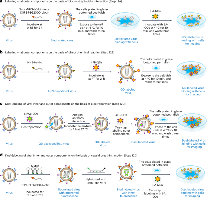
a, Labeling the outer components of biotinylated viruses with SA-QDs via biotin–streptavidin interaction. b, Labeling the outer components of HyNic-modified viruses with 4FB-QDs via direct chemical coupling. c, Labeling the inner components with NPAb-QDs by electroporation followed by labeling of outer components with 4FB-QDs by direct chemical coupling to obtain dual-labeled viruses for imaging. d, Labeling the inner components with MMBs via capsid breathing motion of virus capsid and simultaneous labeling of the outer components with SA-QDs to obtain dual-labeled viruses for imaging.
Table 2 Comparison of the methods for labeling viral outer components Fig. 5: Verification of the labeling efficiency of JEV. 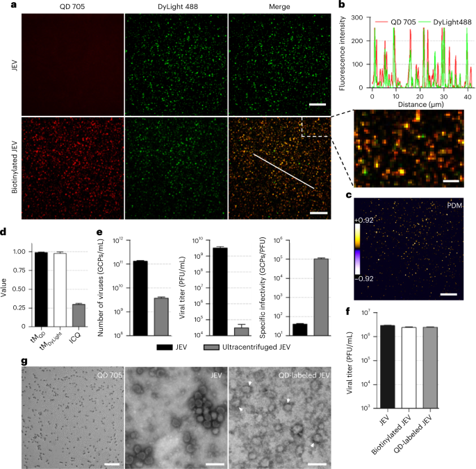
a, Fluorescent images of JEV and biotinylated JEV labeled by SA-QDs (red) via biotin and streptavidin interactions and by anti-E-Dylight 488 (green) via antigen–antibody interactions. Scale bar, 10 μm. The area of dotted line is magnified to clearly show the colocalization of two fluorescence channels. Scale bar, 2 μm. b, Line profile showing colocalization of the red and green signals on the white line in the merged image in a. c, The product of the differences from the mean (PDM) image of the lower merge panel in a. The color code is used to indicate the colocalization extent of two fluorescence channels. Scale bar, 10 μm. d, The Mander’s coefficient (tMQD and tMDyLight) and ICQ values calculated from 20,000 viral particles from three experiments (tMQD, 0.99 ± 0.0078; tMDyLight, 0.98 ± 0.021; ICQ, 0.30 ± 0.014). tMQD denotes the percentage of QD signals colocalized with DyLight signals in the thresholded images, tMDyLight denotes the percentage of DyLight signals colocalized with QD signals in the thresholded images, and ICQ value from 0.5 (colocalization) to −0.5 (exclusion) indicates the colocalization degree of signals. e, Comparison of genome-containing particles (GCPs), viral titers and specific infectivity of wild-type JEV and ultracentrifuged JEV: n = 10 cells from four GCPs, three (viral titers) and four (specific infectivity) independent experiments, respectively. f, Titer of wild-type JEV, biotinylated JEV, SA-QD 705 -labeled JEV. n = 10 cells from three independent experiments. g, TEM images of SA-QD705, JEV and QD-labeled JEV (arrowheads), respectively. Scale bar, 100 nm. Bars represent mean ± s.d. Figure reproduced from ref. 52 under a Creative Commons license CC BY 4.0. Source data.
Critical
Compared with option B, option A is easier to implement and has higher labeling efficiency and less impact on viral infectivity, which is critical for QSVT experiments (Table 2). However, option A requires biotinylated viruses to first bind to receptors on cell membranes and then label the viruses using SA-QDs, resulting in a dynamic process in which the binding of viruses and host cell membrane receptors cannot be monitored. Option B can satisfy the requirements of the above situation. Additionally, option D is easier to implement the dual labeling of viruses for investigating the genome release of viruses in live cells than option C, but cannot be used for investigate the binding dynamics of viruses and host cell membrane receptors. Option C can be used to meet the requirements of the above scenario.
Critical
Once the virus has been labeled, the viral titer (Step 7B or 7C) (Fig. 5e,f) and integrity (Step 7D) (Fig. 5g) of the virus can be examined using the parallel samples of the labeled virus. Virus labeling efficiency can also be checked by performing colocalization experiments (Box 2). In addition, fluorescence spectroscopy, zeta potential and hydrodynamic size experiments can also be performed to initially assess whether the viruses are labeled by QDs53.
Critical step
Filter the solutions containing viruses or SA-QDs to eliminate aggregates before incubation with the cells.
-
(A)
Labeling viral outer components on the basis of biotin–streptavidin interaction
Critical
We present here two methods of biotinylating the outer components of viruses that have little effect on the viral infectivity. Sulfo-NHS-LC-biotin achieves biotinylation of the viral surface by covalent coupling with the amino group on the viral surface, while DSPE-PEG2000-biotin can be inserted into the viral envelope by hydrophobic interaction and is only applicable to enveloped viruses.
-
(i)
Use 100 μL virus suspension (1 mg/mL) and add biotin at a final concentration of 0.1 mg/mL Sulfo-NHS-LC-biotin (or 0.1 mg/mL DSPE-PEG2000-biotin) and incubate for 2 h at RT with shaking.
-
(ii)
Remove the excess biotinylated reagent by using a NAP-5 column, and elute the biotinylated virus from the column with Tyrode’s plus buffer.
-
(iii)
Filter the biotinylated viruses with a 0.22 μm filter to remove the virus aggregates.
-
(iv)
Wash the cells from Step 11 with precooled Tyrode’s plus buffer, add 100 μL biotinylated virus (0.5 mg/mL) and incubate for 10 min at 4 °C.
-
(v)
Aspirate and discard the biotinylated virus suspension and wash the cells three times with precooled Tyrode’s plus buffer, add SA-QDs at a final concentration of 2 nM and incubate for 10 min at 4 °C.
-
(vi)
Wash the treated cells again with precooled Tyrode’s plus buffer to remove the unreacted QDs.
Caution
This cell-based labeling approach, also called the two-step labeling approach, includes multiple washing processes and should be done gently to avoid damaging the cell monolayer on the dish.
-
(vii)
Add 1 mL Tyrode’s plus buffer into the dish and make sure the treated cells are immersed in the buffer solution for imaging immediately.
-
(i)
-
(B)
Labeling viral outer components on the basis of direct chemical coupling
-
(i)
Add 5 μL of 8 μM NH2-QDs (605 nm) and 0.5 mg of NHS-4FB to 45 μL of Tyrode’s plus solution and react for 2 h at RT.
-
(ii)
Remove the excess NHS-4FB by using a NAP-5 column to obtain 4FB-QDs.
-
(iii)
Add 0.1 mg of NHS-HyNic to 100 μL of purified IAV (0.5 mg/mL) and react for 2 h at RT to modify the virus.
Critical step
To verify that viruses have been modified with HyNic, the absorption peak at the absorbance of at 354 nm can be detected using a UV spectrophotometer.
-
(iv)
Remove the excess NHS-HyNic by using a NAP-5 column.
-
(v)
React 1 nM 4FB-QDs with 100 μL of HyNic-modified IAV at RT for 2 h.
-
(vi)
Separate the QD-labeled viruses from the excess 4FB-QDs by sucrose density gradient centrifugation (15−60%), as detailed in Steps 4–6.
-
(vii)
Incubate 100 μL labeled viruses with the treated cells from Step 11 for 10 min at 4 °C.
-
(viii)
Wash the treated cells three times with precooled Tyrode’s plus buffer to remove the unbound viruses.
-
(ix)
Add 1 mL Tyrode’s plus buffer into the dish and make sure the treated cells are immersed in the buffer solution for imaging immediately.
-
(i)
-
(C)
Dual labeling of viral inner and outer components on the basis of electroporation
Critical
Here, we take IAV as an example to label the inner components with NPAb-QDs by antigen–antibody interaction.
-
(i)
Break the disulfide bonds of NPAb by reacting 1 M of DTT with 0.5 mg/mL of NPAb for 0.5 h at RT.
-
(ii)
Remove the excess DTT with a NAP-5 column to acquire reduced NPAb.
-
(iii)
Incubate 4 μM NH2-QDs (525 nm) with 10 mM sulfo-SMCC.
-
(iv)
Remove the excess sulfo-SMCC with a NAP-5 column to obtain activated QDs.
-
(v)
Mix the reduced NPAb with activated QDs, and incubate the mixture at RT for 2 h. Purify the QDs-NPAb conjugates using a Superdex 200 separation column, and concentrate by ultrafiltration to obtain 1.5 μM QDs-NPAb.
-
(vi)
Mix 15 μL of 1 mg/mL IAV with 5 μL QDs−NPAb in 0.1 cm electroporation cuvettes.
-
(vii)
Incubate the mixture for 1 h at 37 °C after eight pulses of electroporation at 500 V/cm, 5 ms duration, 1 Hz frequency to allow NPAb to couple with the viral ribonucleoprotein complex and restore the viral envelope.
-
(viii)
Separate the IAV (containing QDs) from free QDs−NPAb by sucrose density gradient centrifugation as detailed in Steps 4–6.
-
(ix)
Follow the one-step labeling strategy described above (Step 12B) to label the outer components of virus with QDs.
-
(x)
Incubate 100 μL dual-labeled viruses with the treated cells from Step 11 for 10 min at 4 °C.
-
(xi)
Wash the treated cells three times with precooled Tyrode’s plus buffer to remove the unbound viruses.
-
(xii)
Add 1 mL Tyrode’s plus buffer into the dish and make sure the treated cells are immersed in the buffer solution for imaging immediately.
-
(i)
-
(D)
Dual labeling of viral inner and outer components on the basis of capsid breathing motion
Critical
For tracking the genome release during virus infection, some other fluorescent labels that can easily label the viral genome are also recommended as alternative tags. For example, we have used MMBs to label the genome of JEV.10
-
(i)
Add 0.1 mg DSPE-PEG2000-biotin to 100 μL of purified viruses at a concentration of 1 mg/mL, and incubate for 2 h.
-
(ii)
Add 1 μL MMBs (100 nM) into the mixture and shake at 37 °C for 2 h.
-
(iii)
Shield the mixture from light to reduce the influence on the fluorescence of organic dye and shake at 37 °C for 2 h.
-
(iv)
Remove the excess unbounded DSPE-PEG2000-biotin and the MMBs using a NAP-5 desalting column.
-
(v)
Incubate the BHK-21cells with the viruses for 10 min at 4 °C and wash three times with precooled Tyrode’s plus buffer.
-
(vi)
Add 100 μL SA-QDs (2 nM) to the cell-culture dish and incubate at 4 °C for 10 min.
-
(vii)
Wash the cells in the Petri dishes three times with precooled Tyrode’s buffer.
-
(viii)
Add 1 mL Tyrode’s plus buffer in the cell-culture dish for imaging immediately.
-
(i)
-
(A)


Stage 4: image acquisition
Timing 6–8 h
-
13
Place the cells (from Step 12) incubated with the labeled viruses under confocal microscope equipped with CO2 online culture system to obtain the time-series images of the infection process of individual viruses in live cells. The most commonly used tracking method is to track single virus by 2D QSVT (option A). Three-dimensional QSVT (3D QSVT) can also be performed if detailed virus tracking information is required in Z dimensions (option B). In addition, if multiple components of the virus or cell structure need to be labeled, multicolor QSVT can be performed (option C). Figure 6 shows the workflow of 2D, 3D and multicolor QSVT.
Fig. 6: Detailed steps for 2D, 3D and multicolor QSVT. 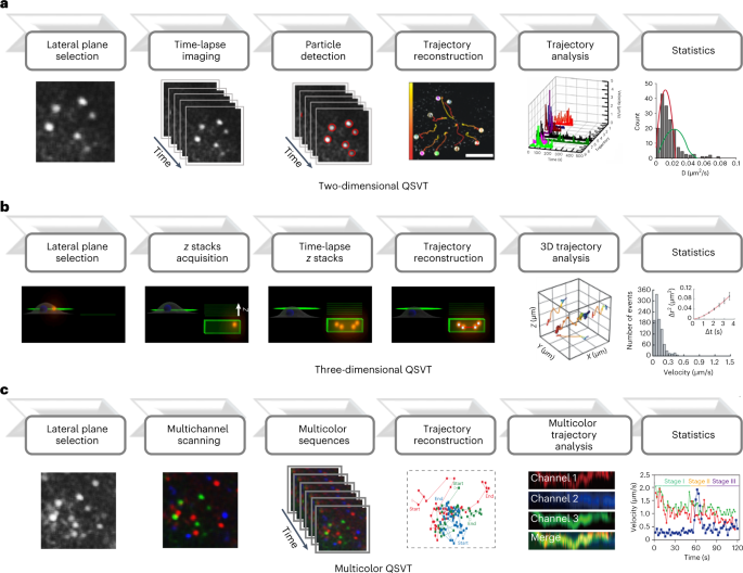
a, Graphics show the procedures of 2D QSVT. Select the lateral plane and perform time-lapse imaging, then detect the particles in the raw image to reconstruct trajectories, and finally conduct statistical analysis of the newly generated trajectories. b, Graphics show the procedures of 3D QSVT. Obtain z-stack images after selecting the lateral plane, then acquire time series of z stacks, reconstruct 3D trajectories and finally perform statistical analysis of 3D trajectories. c, Graphics shows the procedures of multicolor QSVT. Select the lateral plane and perform multichannel scanning, then obtain multicolor sequence of images and finally perform statistical analysis of the reconstructed multicolor trajectories. Images reproduced with permission from: a, ref. 35, American Chemical Society; b, ref. 48, Wiley-VCH. Image adapted with permission from: c, ref. 10, Elsevier.
Critical step
Imaging duration depends on the progression of virus-infected cells, so various types of viruses require different imaging times. In this protocol, imaging times are ~30–90 min for IAV and 30–60 min for JEV. Meanwhile, the live-cell online culture system needs to be turned on 30 min before the start of imaging to maintain proper conditions for virus infection within the live cells.
-
(A)
Performing 2D QSVT
-
(i)
Preview the sample with the camera to obtain the minimal exposure time for imaging individual labeled viruses at high S/N ratios.
-
(ii)
Set the appropriate frame interval with a frame interval less than 500 ms for time-lapse recording.
Caution
QDs are highly photostable, but prolonged exposure to light sources may cause photodamage to cells.
-
(iii)
Acquire fast-time consecutive confocal images (typically ≥500 frames) of the cell.
-
(i)
-
(B)
Performing 3D QSVT
-
(i)
Choose the channel specified in the Z-Scan Control option panel.
-
(ii)
Define Start and End positions to allow the area of interest to be recorded into the scan.
-
(iii)
Set the Z step as 0.3 μm, which is also the size of z-direction pixels.
-
(iv)
Ensure that the frame interval is less than 500 ms after Z reconstruction.
Critical step
To achieve high-speed z-scanning function, we strongly recommend a Prior Nano Scan Z (NZ100CE) for z-sectioning in 3D QSVT.
-
(v)
Acquire a z-stack covering the whole depth of the virus-moving space to obtain 3D images.
Critical step
Although not prohibited, acquisition of z-stacks greater than 0.3 m may result in some loss of fluorescence signal, making long-term tracking of single viruses difficult.
-
(i)
-
(C)
Performing multicolor QSVT
-
(i)
Choose the multichannel imaging settings panel.
-
(ii)
Define the suitable lasers and emission filters for multicolor imaging.
-
(iii)
Set a laser intensity of ~20% and exposure time of ~300 ms for each channel imaging.
-
(iv)
Chose the fluorescent cell of interest in the focal plane, and ensure the frame interval is less than 1 s before recording.
Critical step
The exposure time of each channel should be optimized according to the photostability and brightness of the fluorescent labels.
-
(v)
Acquire fast-time consecutive multichannel confocal images (typically ≥500 frames).
-
(vi)
Save the recorded images and analyze the data when needed.
-
(i)
-
(A)

Stage 5: image processing
Timing 3–6 h
-
14
Extract viral trajectories from 2D QSVT (option A), 3D QSVT (option B) or multicolor QSVT (option C) data.
-
(A)
Extracting the viral trajectory from 2D QSVT data
Critical
Software such as IPP and ImageJ (National Institutes of Health) can be used to process the 2D QSVT images. For ease of use and stability, IPP is strongly recommend and the detailed instructions are as follows:
-
(i)
Import the entire sequence of images into IPP software and convert the sequence of images to 8-bit by selecting Edit > convert to > Gray scale 8, and then select the ‘Best fit’ option.
-
(ii)
Ensure that changes are made to all stacks by selecting the ‘Apply to all stacks’ button on the Sequence tool bar.
-
(iii)
Select Process > Filters > Enhancement > Gauss. Adjust the parameters (e.g., Size, Passes and Strength) in the Option dialogue box below and observe the views in the Sample to obtain an image with a high S/N ratio and maintaining the integrity of the signals. Click the Apply button.
-
(iv)
Regulate the contrast of the image by select Enhance > Contrast enhancement > Brightness/contrast command.
-
(v)
Click the Play button on the Sequence toolbar to check the movements of the particles. Then click the Stop button.
-
(vi)
Open the ‘Tracking Data’ table by selecting Measure > Track Objects.
-
(vii)
Perform either manual particle tracking or automated particle tracking as described in Box 3. Manual particle tracking is suitable for processing images with a small number of particles (≤50), while automatic tracking is suitable for batch analysis with a large number of particles (>50) to obtain a large amount of tracking data more quickly.
-
(i)
-
(B)
Extract the viral trajectory from 3D QSVT data
Critical
For ease of use and stability, Imaris software is strongly recommended to extract the viral trajectory from 3D images. The detailed instructions are as follows:
-
(i)
Import the 3D image sequence into the Imaris software by selecting File > Open > Select file > Open.
-
(ii)
Select Edit > Show Display Adjustment. Adjust the contrast of the image by change the slider bar in the ‘Display Adjustment’ column.
-
(iii)
Select the ‘Surpass’ and ‘3D View’ mode.
-
(iv)
Select the ‘Frame’, ‘Volume’, ‘Spots’ icons in the submenu.
-
(v)
Set the algorithm by selecting Spots > Create > Algorithm Settings > Track Spots (over Time).
-
(vi)
Click the ‘Next: Source Channel’. Set the ‘Estimated XY D’ value according to the size of the particle on the imported image. Click ‘Background Subtraction’.
-
(vii)
Click ‘Next: Classify Spots’. Adjust the slider bar to classify spots.
Critical step
In this column, different filter types can be chosen to classify spots. In general, we recommend to use ‘Quality’ option. Ensure that the particles of interest are selected in this step.
-
(viii)
Click ‘Next: Edit Spots’. Select the ‘all visible’ option.
-
(ix)
Click ‘Next: Tracking’. Set the ‘Tracking Algorithm’ as ‘Connected components’ and ‘Parameters’ according the particle movements.
-
(x)
Click ‘Next: Classify Tracks’. Choose the appropriate filter type to obtain an image with higher S/N ratio while maintaining the integrity of the signal.
-
(xi)
Click ‘Finish: Execute all creation steps and terminate the wizard’ to complete the tracking.
-
(i)
-
(C)
Extract the viral trajectory from multicolor QSVT data
-
(i)
Open the image stacks of a single channel with the Fiji-ImageJ software by selecting File > Import > Image sequence.
Critical step
Split channels by selecting Image > Color > Split channels, if the stacks have multiple color channels.
-
(ii)
Apply the Gaussian blur filter. Select Process > Filters > Gaussian Blur. A panel will appear: deselect the ‘show kernel’ function, and set the Radius (pixels) between 0.5 and 2.0. Click the ‘OK’ button.
Caution
To remove the background noise of the acquired images, many other filters can be used, such as LoPass and Median. A suitable filter should be selected with the aim of obtaining a higher S/N ratio while maintaining the integrity of the signal.
-
(iii)
Draw a line on the first image of the stack passing through the point or region of interest.
-
(iv)
Apply multi kymograph by selecting Analyze > Multi Kymograph > Multi Kymograph.
-
(v)
Set the linewidth between 1.0 and 2.0 on the new pop-up panel. Click the ‘OK’ button.
-
(vi)
Select ‘LUT’ button on the toolbar to color the newly generated image.
-
(vii)
Convert the newly generated image to RGB color by selecting Image > Type > RGB Color.
-
(viii)
Analyze the fluorescent intensity changes by Plot Profile. Draw a line on the RGB color image and then select Analyze > Plot Profile.
-
(ix)
Save the generated kymograph images and Plot Profile results.
-
(i)
-
(A)
Stage 6: data analysis
Timing 3–6 h
Trajectory analysis
-
15
Calculate the instantaneous speeds of the trajectory and plot the instantaneous speed versus time plot to dissect the transport stages during viral infection (Box 4).
-
16
Calculate MSD values at different time lags using the supplementary software, and plot the MSD versus time lag plot to probe the motional mode of virus at different stages (Box 4).
-
17
Analyze the particle intensity versus time plot to investigate the dynamic process of associated protein recruitments during viral infection (Fig. 7).
Fig. 7: Anticipated results of observing the entry of QD-labeled IAV in MDCK cells expressing AcGFP1-Clc by two-color time-lapse imaging. 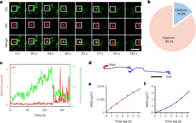
a, Snapshots of the entry of a QDs-labeled (605 nm, red) virus via CME (white squares highlighted) in MDCK cells expressing AcGFP1-Clc (green). Scale bar, 2 μm. b, The proportion of viruses in the internalized virus group (n = 161) that recruited clathrin during entry. c, Fluorescence intensity profile of the clathrin located at virus sites and the velocity profile of virus diffusion shown in a. d, The trajectory of single virus diffusion shown in a. Restriction and orientation phases are shown in red and blue, respectively. Scale bar, 1 μm. e,f, Plots of MSD versus time lag for virus diffusion. The red (e) and blue (f) lines show the fits to the corresponding equations for restricted and directed diffusion, respectively. Figure adapted with permission from ref. 41, American Chemical Society.

Colocalization analysis
-
18
Open the image sequence with different channels into the ImageJ software by selecting File > Import > Image sequence.
Critical step
Make sure the image is 8-bit; if not, select Image > Type > 8-bit.
-
19
Select the ROI containing the fluorescence signals, and crop the image by Image > Crop.
-
20
Denoise with the Gaussian blur filter. Select Process > Filters > Gaussian Blur. A panel will appear: deselect the ‘show kernel’ function, and set the Radius (pixels) between 0.5 and 2.0. Click the ‘OK’ button.
-
21
Apply changes to all slices to the command ‘Yes’.
-
22
Convert stack to images by selecting Image > Stacks > Convert Stack to Images.
-
23
Subtract the background of each image. Select the region of interest (ROI) in the blank area on the image, and perform the background subtraction operation by Plugins > ROI > BG Subtraction from ROI.
-
24
Set the Scaling factor between 1.0 and 3.0, Click the ‘OK’ button.
-
25
Perform colocalization analysis by selecting Plugins > Colocalization Analysis > Intensity Correlation Analysis.
-
26
In the new pop-up panel, set the Crosshair size (pixels) between 2.0 and 3.0, and select ‘Display ICA plots’ and ‘List PDM values’ function. Click the ‘OK’ button.
-
27
Save the data or generated images.
Critical step
The Mander’s coefficient and the intensity correlation quotient (ICQ) values can be acquired to quantitatively analyze the colocalization efficiency.
Troubleshooting
Troubleshooting advice can be found in Table 3.
Timing
-
Steps 1–8, virus amplification and characterization: 4–8 d
-
Steps 9–11, cell labeling and drug inhibition: 1–2 d
-
Step 12, virus labeling: 1–3 d
-
Step 13, image acquisition: 6–8 h
-
Step 14, image processing: 3–6 h
-
Steps 15–27, data analysis: 3–6 h
-
Box 1, drug inhibition: 1–2 h
-
Box 2, colocalization assay: 4–7 h
-
Box 3, 2D QSVT trajectory reconstruction: 1–3 h
Anticipated results
The protocol provides details of virus amplification and labeling methods, as well as the implementation of QSVT experiments. By carefully following the protocol, the dynamic infection behavior of individual viruses and the transient molecular events associated with virus–host cell interactions in living cells can be visualized and analyzed in real time.
Figure 7 shows the anticipated results of observing QD-labeled IAV entry in MDCK cells expressing AcGFP1-Clc by two-color time-lapse imaging (Fig. 7a)41. We analyzed the trajectory of the virus moving from the plasma membrane to the perinuclear region, the time-dependent instantaneous speed of the virus and the fluorescence intensity of the corresponding AcGFP1-labeled clathrin-coated structures (Fig. 7c,d). The fluorescence intensity of clathrin gradually increased with increasing time of virus infection and reaches a peak after a certain time, indicating that clathrin recruitment occurs at the binding site of the virus on the cell membrane, which is also an indicator of the initiation of clathrin-coated pits (CCP). Analysis of MSD versus time lag plots revealed that during clathrin recruitment, the virus underwent mainly slow (~0.1 μm/s) and restricted diffusion movements (Fig. 7e), indicating that the virus was confined to the binding site while CCPs were being produced and grown. Then, the dramatic decrease and eventual disappearance of clathrin fluorescence, followed by rapid movement of the virus toward the cytoplasm, suggests that clathrin-coated vesicles are able to rapidly depolymerize before the virus is transported to the cytoplasm. The rapid movement of the virus (>0.5 μm/s) is consistent with motor-driven directional diffusion and represents cytoskeleton-dependent transport of the virus-containing vesicles (Fig. 7f). Statistical results showed that ~85% of the internalized viruses (137/161 in 20 cells) were ensnared during clathrin recruitment (Fig. 7b), suggesting that IAV tends to trigger and hijack clathrin-mediated endocytosis (CME) for their entry.
Figure 8 shows the anticipated results when JEV virus infection of BHK cells was studied by QSVT technique10. Confocal imaging showed that the virus was mainly distributed around the plasma membrane after incubation with BHK-21 cells at 4 °C for 10 min (Fig. 8a). After initiating infection at 37 °C for 20 min, the viruses were observed to accumulate in the inner regions of the cells. As the infection time increased, more virus particles entered the cytoplasm of the cells. Also, by 60 min of infection, 80% of the viral particles within the cytoplasm underwent separation of envelope and RNA genomic signals. Figure 8b,c illustrates a typical viral track that starts at the cell periphery, moves toward the nucleus and releases its genome in the perinuclear region. Examining the instantaneous speed versus time curve of the virus found that the entire infection process of JEV follows a distinct slow-fast-slow movement pattern (Fig. 8d). The virus initially moves slowly in the cell periphery (stage I), then rapidly and directionally move toward the nucleus (stage II), followed by a bidirectional and intermittent movement near the nucleus before genome release (stage III). The fluorescence signal of the labeled genome can still be detected at the single-virus level throughout the infection (Fig. 8e). The distribution of instantaneous speed and MSD versus time lag curves of the viral movement at each stage confirmed that JEV moved from the cell periphery to the perinuclear region along actin filaments and microtubules before genome release (Fig. 8f–h). In contrast, after using Cyto-D or nocodazole to disrupt microfilaments and microtubules for 60 min, respectively, the motilities of the viruses were significantly restricted and the circle radiuses became greatly reduced in the treated cells, demonstrating that JEV is transported from the cell membrane to the nucleus via actin filament and microtubule.

a, Postinfection images of live BHK-21 cells infected by dual-labeled JEVs at different timepoints (n = 50). The viral envelope is labeled by 625 nm QDs (green) and viral genome is labeled by Cy5-modified multiple molecular beacons (red). Fluorescence colocalization (yellow) demonstrates that genome release has not occurred. Scale bar, 10 µm. Zoomed images of white dotted boxes shown in the merged images. Scale bar, 5 µm. b, Display of a typical trajectory of a single dual-labeled virus that moved from the periphery of BHK-21 cell toward the perinuclear region. Trajectory are coded with color bars representing a consistent timeline from 0 s to 120 s. It is highlighted by a white dotted line for the nucleus and a white dashed line for the cell boundary. Scale bar, 2 µm. c, Time-lapse images of the single JEV particle (white arrows) shown in b. Scale bar, 200 nm. d, The instantaneous velocity plot of the virus motion trajectory in b. According to the instantaneous velocity, the movement of the virus can be divided into three phases (phases I, II and III). e, Fluorescence intensity plot of the viral genome (red) and envelope (green) following the trajectory shown in b. f–h, Frequency distribution plots of instantaneous virus velocity for stages I, II and III. The inset shows the MSD versus time lag plots of the viruses in the three phases (n = 3). The lines are fits to the MSD = 4Dt + (Vt)2 + constants, D = 0.008 μm2/s (f), 0.012 μm2/s (g) and 0.011 μm2/s (h); V = 0.07 μm/s (f), 0.27 μm/s (g) and 0.12 μm/s (h). D and V are the diffusion coefficient and the fitted velocity, respectively, and the constant is attributed to the noise. i, One movement trajectory for 150 s extracted from the untreated, Cyto-D-treated and nocodazole-treated cells, respectively. j, Mean circle radius of movement trajectories extracted from untreated, Cyto-D-treated and nocodazole-treated cells (n = 20). Bars represent mean ± s.d. Statistical analysis was performed using unpaired two-sample t-test; ⋆⋆⋆P < 0.001. Figure adapted with permission from ref. 10, Elsevier.
Code availability
All the MSD calculation code used in this study is available in the Supplementary Software.
References
Marsh, M. & Helenius, A. Virus entry: open sesame. Cell 124, 729–740 (2006).
Greber, U. F. & Way, M. A superhighway to virus infection. Cell 124, 741–754 (2006).
Liu, S. L. et al. Single-virus tracking: from imaging methodologies to virological applications. Chem. Rev. 120, 1936–1979 (2020).
Brandenburg, B. & Zhuang, X. Virus trafficking–learning from single-virus tracking. Nat. Rev. Microbiol. 5, 197–208 (2007).
Wang, Z. G., Liu, S. L. & Pang, D. W. Quantum dots: a promising fluorescent label for probing virus trafficking. Acc. Chem. Res. 54, 2991–3002 (2021).
Yang, Y. B. et al. Single virus tracking with quantum dots packaged into enveloped viruses using CRISPR. Nano Lett. 20, 1417–1427 (2020).
Pinaud, F., Clarke, S., Sittner, A. & Dahan, M. Probing cellular events, one quantum dot at a time. Nat. Methods 7, 275–285 (2010).
Resch-Genger, U., Grabolle, M., Cavaliere-Jaricot, S., Nitschke, R. & Nann, T. Quantum dots versus organic dyes as fluorescent labels. Nat. Methods 5, 763–775 (2008).
Zhang, L. J. et al. A ‘driver switchover’ mechanism of influenza virus transport from microfilaments to microtubules. ACS Nano 12, 474–484 (2018).
Liu, H. Y. et al. In-situ quantitation of genome release of Japanese encephalitis viruses by quantum dot-based single-virus tracking. Nano Today 40, 101271 (2021).
Wang, Z. G. et al. Spatiotemporal quantification of endosomal acidification on the viral journey. Small 18, e2104200 (2022).
Ma, Y. et al. Quantum dot nanobeacons for single RNA labeling and imaging. J. Am. Chem. Soc. 141, 13454–13458 (2019).
Nathan, L. & Daniel, S. Single virion tracking microscopy for the study of virus entry processes in live cells and biomimetic platforms. Adv. Exp. Med. Biol. 1140, 13–43 (2019).
Li, Q. et al. Encapsulating quantum dots within HIV-1 virions through site-specific decoration of the matrix protein enables single virus tracking in live primary macrophages. Nano Lett. 18, 7457–7468 (2018).
Seisenberger, G. et al. Real-time single-molecule imaging of the infection pathway of an adeno-associated virus. Science 294, 1929–1932 (2001).
Lakadamyali, M., Rust, M. J., Babcock, H. P. & Zhuang, X. Visualizing infection of individual influenza viruses. Proc. Natl Acad. Sci. USA. 100, 9280–9285 (2003).
van der Schaar, H. M. et al. Dissecting the cell entry pathway of dengue virus by single-particle tracking in living cells. PLoS Pathog. 4, e1000244 (2008).
Rust, M. J., Lakadamyali, M., Zhang, F. & Zhuang, X. Assembly of endocytic machinery around individual influenza viruses during viral entry. Nat. Struct. Mol. Biol. 11, 567–573 (2004).
van der Schaar, H. M. et al. Characterization of the early events in dengue virus cell entry by biochemical assays and single-virus tracking. J. Virol. 81, 12019–12028 (2007).
McDonald, D. et al. Visualization of the intracellular behavior of HIV in living cells. J. Cell Biol. 159, 441–452 (2002).
Miyauchi, K., Kim, Y., Latinovic, O., Morozov, V. & Melikyan, G. B. HIV enters cells via endocytosis and dynamin-dependent fusion with endosomes. Cell 137, 433–444 (2009).
Koch, P. et al. Visualizing fusion of pseudotyped HIV-1 particles in real time by live cell microscopy. Retrovirology 6, 84 (2009).
Hendrix, J. et al. Live-cell observation of cytosolic HIV-1 assembly onset reveals RNA-interacting gag oligomers. J. Cell Biol. 210, 629–646 (2015).
Baumgartel, V. et al. Live-cell visualization of dynamics of HIV budding site interactions with an ESCRT component. Nat. Cell Biol. 13, 469–474 (2011).
Ivanchenko, S. et al. Dynamics of HIV-1 assembly and release. PLoS Pathog. 5, e1000652 (2009).
Xing, Y. et al. Bioconjugated quantum dots for multiplexed and quantitative immunohistochemistry. Nat. Protoc. 2, 1152–1165 (2007).
Wang, Z. G. et al. Real-time dissecting the dynamics of drug transportation in the live brain. Nano Lett. 21, 642–650 (2021).
Zhang, L. J., Xia, L., Xie, H. Y., Zhang, Z. L. & Pang, D. W. Quantum dot based biotracking and biodetection. Anal. Chem. 91, 532–547 (2019).
Medintz, I. L., Uyeda, H. T., Goldman, E. R. & Mattoussi, H. Quantum dot bioconjugates for imaging, labelling and sensing. Nat. Mater. 4, 435–446 (2005).
Zhang, F. et al. Self-biotinylation and site-specific double labeling of baculovirus using quantum dots for single-virus in-situ tracking. Biomaterials 34, 7506–7518 (2013).
Joo, K.-I. et al. Site-specific labeling of enveloped viruses with quantum dots for single virus tracking. ACS Nano 2, 1553–1562 (2008).
Joo, K. I. et al. Enhanced real-time monitoring of adeno-associated virus trafficking by virus-quantum dot conjugates. ACS Nano 5, 3523–3535 (2011).
Zhang, Y. et al. Encapsulating quantum dots into enveloped virus in living cells for tracking virus infection. ACS Nano 7, 3896–3904 (2013).
Zhang, P. et al. Click-functionalized compact quantum dots protected by multidentate-imidazole ligands: conjugation-ready nanotags for living-virus labeling and imaging. J. Am. Chem. Soc. 134, 8388–8391 (2012).
Liu, S. L. et al. Effectively and efficiently dissecting the infection of influenza virus by quantum-dot-based single-particle tracking. ACS Nano 6, 141–150 (2012).
Liu, H., Liu, Y., Liu, S., Pang, D. W. & Xiao, G. Clathrin-mediated endocytosis in living host cells visualized through quantum dot labeling of infectious hematopoietic necrosis virus. J. Virol. 85, 6252–6262 (2011).
Qin, C. et al. Real-time dissection of dynamic uncoating of individual influenza viruses. Proc. Natl Acad. Sci. USA 116, 2577–2582 (2019).
Ma, Y. et al. Live cell imaging of single genomic loci with quantum dot-labeled TALEs. Nat. Commun. 8, 15318 (2017).
Bao, M.-N. et al. Influenza A viruses enter host cells via extracellular Ca2+ influx-involved clathrin-mediated endocytosis. ACS Appl. Bio. Mater. 4, 2044–2051 (2021).
Lv, C. et al. Internalization of the pseudorabies virus via macropinocytosis analyzed by quantum dot-based single-virus tracking. Chem. Commun. 54, 11184–11187 (2018).
Sun, E. Z. et al. Real-time dissection of distinct dynamin-dependent endocytic routes of influenza A virus by quantum dot-based single-virus tracking. ACS Nano 11, 4395–4406 (2017).
Tang, B. et al. Sphingomyelin-sequestered cholesterol domain recruits formin-binding protein 17 for constricting clathrin-coated pits in influenza virus entry. J. Virol. 96, e01813–e01821 (2022).
Wu, Q. M. et al. Uncovering the Rab5-independent autophagic trafficking of influenza A virus by quantum-dot-based single-virus tracking. Small 14, e1702841 (2018).
Wen, L. et al. Intracellular self-assembly based multi-labeling of key viral components: envelope, capsid and nucleic acids. Biomaterials 99, 24–33 (2016).
Hong, Z. Y. et al. Clicking hydrazine and aldehyde: the way to labeling of viruses with quantum dots. ACS Nano 9, 11750–11760 (2015).
Wen, L. et al. Labeling the nucleocapsid of enveloped baculovirus with quantum dots for single-virus tracking. Biomaterials 35, 2295–2301 (2014).
Liu, S. L. et al. High-efficiency dual labeling of influenza virus for single-virus imaging. Biomaterials 33, 7828–7833 (2012).
Wang, Z. G. et al. Exploring sialic acid receptors-related infection behavior of avian influenza virus in human bronchial epithelial cells by single-particle tracking. Small 10, 2712–2720 (2014).
Liu, S. L. et al. Fast and high-accuracy localization for three-dimensional single-particle tracking. Sci. Rep. 3, 2462 (2013).
Liu, S. L. et al. Globally visualizing the microtubule-dependent transport behaviors of influenza virus in live cells. Anal. Chem. 86, 3902–3908 (2014).
Liu, S. L. et al. Three-dimensional tracking of Rab5- and Rab7-associated infection process of influenza virus. Small 10, 4746–4753 (2014).
Zhang, L. J. et al. Lipid-specific labeling of enveloped viruses with quantum dots for single-virus tracking. mBio 11, e00135–20 (2020).
Hong, Z. Y. et al. Equipping inner central components of influenza a virus with quantum dots. Anal. Chem. 90, 14020–14028 (2018).
Eisfeld, A. J., Neumann, G. & Kawaoka, Y. Influenza A virus isolation, culture and identification. Nat. Protoc. 9, 2663–2681 (2014).
Acknowledgements
This work was supported by the National Key Research and Development Program of China (2019YFA0210500) and by the National Natural Science Foundation of China (Nos.91859123, 21877102, 21977054 and 91953107). We thank the Haihe Laboratory of Sustainable Chemical Transformations for financial support.
Author information
Authors and Affiliations
Contributions
D.-W.P. is the group leader and conceived and initiated the project, and supervised the study and the entire manuscript preparation; S.-L.L., Z.-G.W. and H.-Y.L. developed the procedures for virus labeling and data processing. H.-Y.L. and Z.-G.W. organized and wrote the manuscript. All authors reviewed and edited the manuscript and approved the final draft.
Corresponding author
Ethics declarations
Competing interests
The authors declare no competing interests.
Peer review
Peer review information
Nature Protocols thanks Chengzhi Huang, Fei Liu and the other, anonymous, reviewer(s) for their contributions to the peer review of this work.
Additional information
Publisher’s note Springer Nature remains neutral with regard to jurisdictional claims in published maps and institutional affiliations.
Related links
Key references using this protocol
Sun, E. Z. et al. ACS Nano 11, 4395–4406 (2017): https://doi.org/10.1021/acsnano.6b07853
Liu, H. Y. et al. Nano Today 40, 101271 (2021): https://doi.org/10.1016/j.nantod.2021.101271
Zhang, L. J. et al. mBio 11, e00135-20 (2020): https://doi.org/10.1128/mBio.00135-20
Supplementary information
Supplementary Software 1
Calculating mean square displacement (MSD) result of provided trajectory, generating fitted MSD colored curve, generating particle velocity versus frame interval colored curves.
Source data
Source Data Fig. 5
Statistical source data for Fig. 5d–f.
Source Data Fig. 8
Statistical source data for Fig. 8j.
Rights and permissions
Springer Nature or its licensor (e.g. a society or other partner) holds exclusive rights to this article under a publishing agreement with the author(s) or other rightsholder(s); author self-archiving of the accepted manuscript version of this article is solely governed by the terms of such publishing agreement and applicable law.
About this article

Cite this article
Liu, HY., Wang, ZG., Liu, SL. et al. Single-virus tracking with quantum dots in live cells. Nat Protoc 18, 458–489 (2023). https://doi.org/10.1038/s41596-022-00775-7
Received:
Accepted:
Published:
Issue Date:
DOI: https://doi.org/10.1038/s41596-022-00775-7
Comments
By submitting a comment you agree to abide by our Terms and Community Guidelines. If you find something abusive or that does not comply with our terms or guidelines please flag it as inappropriate.
