Quantum fluctuation of ferroelectric order in polar metals

Abstract

The polar metallic phase is an unusual metallic phase of matter containing long-range ferroelectric (FE) order in the electronic and atomic structure. Distinct from the typical FE insulating phase, this phase spontaneously breaks the inversion symmetry without global polarization. Unexpectedly, the FE order is found to be dramatically suppressed and destroyed at moderate ~ 10% carrier density. Here, we propose a general mechanism based on carrier-induced quantum fluctuations to explain this puzzling phenomenon. The quantum kinetic effect would drive the formation of polaronic quasi-particles made of the carriers and their surrounding dipoles. The disruption in dipolar directions can therefore weaken or even destroy the FE order. We demonstrate such polaron formation and the associated FE suppression via a concise model using exact diagonalization, perturbation, and quantum Monte Carlo approaches. This quantum mechanism also provides an intuitive picture for many puzzling experimental findings, thereby facilitating new designs of multifunctional FE electronic devices augmented with quantum effects.

Introduction

Ferroelectric (FE) order corresponds to an ordering of local electric dipole moment in materials associated with a spontaneously broken inversion symmetry in the absence of an external electric field. Accordingly, insulating FE materials typically exhibit a field-switchable global spontaneous polarization (P) and consequently a rather strong dielectric response. This feature makes FE materials highly functional in electronic devices and other practical applications, including energy storage^1,2,3, photovoltaics^4,5,6,7, data storage and switching⁸. In recent years, the attempt to functionalize FE materials with additional metallicity has stimulated intensive studies of the so-called “polar metal” phase in charge carrier-doped FE materials, which hosts metallic carriers in the presence of FE order.

Such a FE metallic “polar metal” state was first predicted by Anderson and Blount⁹, who theorized broken inversion symmetry along a polar axis and the persistence of FE-like phase transitions in this metallic phase. It was not until 2013 the polar metallic state was finally discovered in LiOsO₃ by Shi et al.¹⁰. Since then, many polar metals have been found in various carrier-doped FE materials¹¹, including perovskite oxides: BaTiO₃^{12,13,14,15,16}, Sr_1−xCa_xTiO₃¹⁷, PbTiO₃^18,19, CaTiO₃²⁰; NdNiO₃²¹, LiOsO₃^10,22, Ca₃Ru₂O₇²³, and Cd₂Re₂O₇²⁴; hexagonal FE materials: LiGaGe²⁵ and LaAuGe²⁶; and 2D layered materials: WTe₂^27,28 and MoTe₂²⁹. These polar metals are also found to display rich physical properties^12,14,30,31, showing unusual transport properties^17,32,33 and even exotic superconductivity^34,35.

In polar metallic phase, as shown in phase II of Fig. 1, charge carriers can propagate freely in materials as soon as the global P and correspondingly the total electric field E is fully screened by δ_c1 ~ 2% of carriers accumulating on the domain boundaries and surfaces^36,37. On the other hand, the FE order having a spontaneously broken symmetry still exists up to δ_c2 ~ 10%^{12,13,14,16,18,20,23,24}, despite the absence of the global P. Naturally, with the screening of the beneficial E, ferroelectricity is expected to be weakened as widely found in current observations, for example, a decrease in phase transition temperatures (T_c) and coercive field (E_c)^{12,13,14,32,38,39}, a remarkably reduced off-center FE distortions^12,13,14, a softening of the soft mode phonon³⁹ and an emergence of the over-damped highly-anharmonic central mode^39,40.

Fig. 1: Schematic phase diagrams of three phases in electron-doped FE materials upon increasing carrier density δ.

a Illustrates the macroscopic properties, such as the global dipole P and the FE order parameter o. b Demonstrates the underlying microscopic properties, including spatial distribution of electronic density of states and electric dipole at different stages of the phase diagram. Stage I (FE insulator): with a tiny amount of doped electrons, charges are exhausted to screen the electric field E and the global dipole P by accumulating at the surface of the materials (or domain boundary). Stage II (polar metal): with enough electrons to fully screen the electric field E, some portion of the doped carriers can propagate in the system, while the FE order (characterized via order parameter o) corresponding to the non-centrosymmetric electronic and atomic structure remains. Stage III (paraelectric metal): with even more carriers introduced to the system, the FE order is also destroyed and the surface charge is released to join the itinerant carriers.

There are however, many unexpected puzzling behaviors in this phase, associated with the introduction of metallic carriers, including an anomalous sign reversal in the Hall coefficient in n-doped BaTiO₃ single crystal³², a remarkably low carrier scattering rate, a modest intrinsic carrier mobility³³, and a sudden increase in the real part of the dielectric function in sub-THz region in lead halide perovskites^30,31. Even more unusual is that the observed transition temperature of the lowest-temperature FE phase appears to be nearly doping independent¹², or even slightly increasing with doping in n-doped BaTiO₃¹⁴, despite the overall weakening of the FE order.

Still, the most puzzling is why in this phase the FE order can be so efficiently suppressed by merely ~ 10% of doping, particularly when the global P and E are already fully compensated in the entire phase. As shown in Fig. 1, apart from accumulating at the FE surface/domain boundary to screen the E field, the carriers also propagate in the field-free region in this phase. Intuitively, when residing in the center atom inside an octahedral cage, each carrier can enlarge the atomic size and thus remove the local polar distortion and its associated local dipole moment p. However, it is not obvious how merely ~ 10% of depletion of local dipoles can destroy so effectively the long-range order of the entire system, characterizable via an order parameter o proportional to, for example, the average local dipole moment 〈p〉. This strange phenomenon clearly reflects the fundamental nature of the polar metallic state. A proper microscopic understanding of it would surely provide the basis for a natural explanation of other puzzles above and pave the way for further engineering and optimization of these functional materials.

This puzzling behavior, however, poses a clear challenge to current pictures of polar metallic phase. The common mesoscopic classical picture of nanometer-scale domain mixture¹³ and the observation of ‘diffusive’ phase transition^41,42 provide no mechanism directly, particularly considering the rather small amount of impurities and the associated disorder effects. Another popular scenario that leads to successful geometric design^20,21,43, the so-called ‘weak coupling hypothesis’⁴⁴ between the carrier and the FE order, is obviously not applicable to address the efficient destruction of the latter via the introduction of the former. Similarly, density functional studies^45,46 or perturbation treatments⁴⁷ assume very large time-scale separation of electron and lattice dynamics, directly contradicting the observed really low carrier mobility³³. Even more specific picture aiming to address this particular issue, for example, consideration based on carriers’ screening of supposedly beneficial long-range interaction²⁰ encounters difficulty since the long-range interaction was shown unnecessary to establish a stable FE order^48,49. In fact, classical pictures⁵⁰ would generically have fundamental difficulty circumventing the thermodynamical requirement of entropy reduction at low temperatures, which instead promotes ordering even with the introduction of itinerant carriers.

Here, we propose a general mechanism for the efficient suppression of the FE order in the polar metallic phase through its quantum fluctuation, associated with the generic formation of itinerant “polarons”. As illustrated in Fig. 2 and quantified below, the kinetic process of quantum carrier that allows it to move between atoms can naturally lead to a superposition of disoriented dipoles in its vicinity. Such a high-energy (fast) process would ensure a rigid local structure of the carrier and its surrounding disturbed dipoles at low energy (longer time scale) relevant to the transport properties or broken symmetry phase of these polar metallic materials. It is therefore convenient to regard the resulting local structure as a new emergent mobile particle named polaron. Since the dipoles are disrupted within, large mobile polarons can thus efficiently weaken or destroy the long-range FE order even at low carrier density, as observed experimentally. In great contrast to the classical pictures, the quantum superposition of disoriented dipoles indicates multiple possible directions of each dipole even at zero temperature, since a coherent superposition carries no internal entropy. We demonstrate below the formation of such a quantum polaron and its disrupting effects on FE order with a simple model using exact diagonalization, perturbation, and world-line quantum Monte Carlo. The proposed quantum mechanism can offer natural explanations to many other anomalous experimental findings in polar metals. Particularly, the explicit inclusion of quantum physics should prove essential in understanding and engineering polar metals in general.

Fig. 2: Schematic of the spatial structure of polarons.

In polar metallic phase, itinerant low-energy carriers are slow emergent quasi-particles named “polarons” made of charge centers and fluctuating local dipoles surrounding them. Such polarons acquire their internal structure via fast dynamics of the charge that disrupts the orientation of nearby local dipoles, a process commonly referred to as quantum fluctuation.

To demonstrate the quantum mechanical formation of polaron in carrier-doped FE materials and its essential properties, let us consider a general model hosting a strong coupling between the electronic and atomic lattice degrees of freedom. As illustrated in Fig. 3a, in each octahedron, their local structure is simplified to one of the few low-energy local states resulting from some high-energy physical mechanisms. (See Method section for more details.) Specifically in the absence of itinerant carriers, the local electronic and atomic structure at a particular octahedron site, i, would be in a local symmetry-broken state, ${a}_{in}^{{\dagger} }\left\vert 0\right\rangle$ (in second quantized notation) that hosts an electric dipole along one of the energetically favored directions with a fixed moment size p₀, for example, n = 1, 2, ⋯ , 8 corresponding to one of the eight 〈111〉 directions, $\hat{{{{\bf{n}}}}}$, toward the face centers of a TiO₆ octahedron in BaTiO₃. In contrast, with an itinerant carrier in the octahedron, the local electronic and atomic structure would instead be in a locally symmetric charged state, ${c}_{i}^{{\dagger} }\left\vert 0\right\rangle$, as a result of the enlarged size of the central cation from its additional charge. The simplest but rather generic effective Hamiltonian then reads,

$$\begin{array}{lll}H&=&{H}_{t}+{H}_{MD}+{H}_{DD}+{H}_{R}\\ &=&\mathop{\sum}\limits_{i{i}^{{\prime} }n{n}^{{\prime} }}{t}_{i{i}^{{\prime} }}{({a}_{in}^{{\dagger} }{c}_{i})}^{{\dagger} }({a}_{{i}^{{\prime} }{n}^{{\prime} }}^{{\dagger} }{c}_{{i}^{{\prime} }})+\mathop{\sum}\limits_{i{i}^{{\prime} }{n}^{{\prime} }}{K}_{i,{i}^{{\prime} }{n}^{{\prime} }}{c}_{i}^{{\dagger} }{c}_{i}{a}_{{i}^{{\prime} }{n}^{{\prime} }}^{{\dagger} }{a}_{{i}^{{\prime} }{n}^{{\prime} }}\\ &&-\, \mathop{\sum}\limits_{i{i}^{{\prime} }n{n}^{{\prime} }}{J}_{in,{i}^{{\prime} }{n}^{{\prime} }}{a}_{in}^{{\dagger} }{a}_{in}{a}_{{i}^{{\prime} }{n}^{{\prime} }}^{{\dagger} }{a}_{{i}^{{\prime} }{n}^{{\prime} }}+\mathop{\sum}\limits_{in{n}^{{\prime} }}{R}_{n{n}^{{\prime} }}{a}_{in}^{{\dagger} }{a}_{i{n}^{{\prime} }},\end{array}$$

(1)

where ${c}_{i}^{{\dagger} }({c}_{i})$ and ${a}_{in}^{{\dagger} }({a}_{in})$ follow fermionic and bosonic statistics, respectively. Since each octahedron site can only host either one of the dipole modes or one with a carrier, they follow the strict single-choice exclusion condition,

$$\left\{\begin{array}{l}{c}_{i}^{{\dagger} }{a}_{in}^{{\dagger} }={a}_{in}^{{\dagger} }{a}_{i{n}^{{\prime} }}^{{\dagger} }=0\\ {c}_{i}^{{\dagger} }{c}_{i}+\sum\limits_{n}{a}_{in}^{{\dagger} }{a}_{in}=1.\end{array}\right.$$

(2)

Fig. 3: Illustration of the quantum states and the quantum kinetic process in our model.

a Nine possible local low-energy states of an octahedron site i, either with a dipole in one of the eight preferred directions, or with a charged carrier. b Before the electron is introduced, the local dipoles are well aligned along the ordered direction in the many-body state $\left\vert {{{\Phi }}}_{0}\right\rangle$. c Upon introduction of an electron, in the many-body state $\left\vert {{{\Phi }}}_{1}\right\rangle$ the local octahedron containing one more charge will be in the charged mode without a local dipole, effectively removing the original dipole mode upon carrier addition, ${({a}_{in}^{{\dagger} }{c}_{i})}^{{\dagger} }$. (d) When the electron propagates to the neighboring octahedron through the kinetic processes ${t}_{i{i}^{{\prime} }}{({a}_{in}^{{\dagger} }{c}_{i})}^{{\dagger} }({a}_{{i}^{{\prime} }{n}^{{\prime} }}^{{\dagger} }{c}_{{i}^{{\prime} }})$, it leaves behind a dipolar mode in one of the possible directions in the many-body state $\left\vert {{{\Phi }}}_{2}\right\rangle$. As shown in d, a quantum polaron state contains linear superposition (illustrated by multi-directional arrows) of all possible such quantum fluctuations in its vicinity.

The third term H_DD of Eq. (1) is simply the second quantized representation of the familiar inter-site dipole-dipole coupling, ${H}_{DD}=-{\sum }_{i,{i}^{{\prime} }}\left({J}_{i{i}^{{\prime} }}/{p}_{0}^{2}\right){{{{\bf{p}}}}}_{i}\cdot {{{{\bf{p}}}}}_{{i}^{{\prime} }}$, between dipole moments ${{{{\bf{p}}}}}_{i}={p}_{0}{\sum }_{n}\hat{{{{\bf{n}}}}}{a}_{in}^{{\dagger} }{a}_{in}$. Similarly, the second term H_MD represents the monopole-dipole coupling, ${H}_{MD}=-{\sum }_{i,{i}^{{\prime} }}\left({K}_{i{i}^{{\prime} }}/{p}_{0}\right){\hat{{{{\bf{r}}}}}}_{i{i}^{{\prime} }}\cdot {{{{\bf{p}}}}}_{{i}^{{\prime} }}$, between the charged carrier and the surrounding dipoles³¹ along the direction of relative position ${\hat{{{{\bf{r}}}}}}_{i{i}^{{\prime} }}=\left({{{{\bf{r}}}}}_{i}-{{{{\bf{r}}}}}_{{i}^{{\prime} }}\right)/| {{{{\bf{r}}}}}_{i}-{{{{\bf{r}}}}}_{{i}^{{\prime} }}|$. The last term H_R describes the intrinsic fluctuation between dipole modes corresponding to the switch of the local dipole directions.

The intriguing physics introduced by itinerant carriers is mostly through its quantum mechanical kinetic effect given by the first term, ${H}_{t}={\sum }_{i{i}^{{\prime} }n{n}^{{\prime} }}{t}_{i{i}^{{\prime} }}{({a}_{in}^{{\dagger} }{c}_{i})}^{{\dagger} }({a}_{{i}^{{\prime} }{n}^{{\prime} }}^{{\dagger} }{c}_{{i}^{{\prime} }})$. It describes the ‘bare’ hopping of an itinerant carrier from a site ${i}^{{\prime} }$ to a neighboring site i and thereby removing the dipole at site i. As described/enforced by the single-choice exclusion constraint, Eq. (2), this process also leave behind an uncharged site ${i}^{{\prime} }$ that must then develop a dipole. A key aspect of quantum mechanics is that the newly developed dipole can in principle be in any possible modes ${n}^{{\prime} }$, or more generally in a quantum superposition of them shown in Fig. 3d. As to be demonstrated in the results below, this feature is the essential ingredient for the quantum fluctuation of FE order inside the polarons.

Note that Eq. (1) is specifically meant to capture the eV-scale physics that establishes robust local polarons. It therefore does not include many of the low-energy (sub-eV scale, slow) processes, for example, the small fluctuation of dipoles near each stable mode due to the 20 meV-scale phononic vibration of the atoms⁵¹, or even slower ~4 meV-scale domain wall dynamics of depolarization field⁵². For a similar reason, very high-energy (multiple-eV scale, rapid) dynamics beyond the scale of polaronic formation have been conceptually decoupled from Eq. (1) through renormalizing the remaining physical effects in Eq. (1). For example, one might wonder about the dynamical process corresponding to the disappearance/emergence of local dipoles associated with charge addition/removal to the local transitional metal sites However, since this involves a large beyond-eV scale Coulomb energy change, for the eV-scale physics described by Eq. (1) the influence of very high-energy physics is absorbed and contributes to the strength of the remaining effective parameters.

Below we will study the structure of a single polaron using three numerical calculations: exact diagonalization, perturbation theory, and world-line quantum Monte Carlo (QMC). The first two provide a clear picture of the polaron formation and kinetic energy dependence of the polaron size, while the third reveals additional effects of polaron motion on quantum fluctuation. To demonstrate more cleanly the purely quantum kinetic effect, the classical monopole-dipole term H_MD is dropped in our calculation. This simplification slightly weakens the quantum fluctuation but does not modify our result qualitatively. Without loss of generality, only nearest neighbors are included in H_t and H_DD as well. Furthermore, for the prototypical BaTiO₃ derived polar metals of interest here, the dipolar switch rate in H_R is orders of magnitude smaller than H_t and H_DD and is thus neglected. (See the Methods section for a detailed discussion on these simplifications.)

Results

Formation and internal structure of quantum polarons

Figure 4a demonstrates the structure of a quantum polaron from the ground state of our exact diagonalization and perturbation calculation. It shows a density distribution of a quantum state describing the real charge carriers relevant to the slow transport process. This carrier has a well-defined location, and its density extends to surrounding atoms. Importantly, in each contribution to the superposition of the quantum state of a polaron, the local electric dipoles (not shown in Fig. 4) within the scope of this extension are disrupted from the FE order 〈O〉 (so-called “quantum fluctuation”). In other words, polarons indeed would form in a polarizable media consisting of particles and their nearby disrupted local dipoles.

Fig. 4: Spatial structure of the polaron and its disruption on the local dipoles.

a The site-distribution of charge density, ${\rho }_{i}\equiv \langle {c}_{i}^{{\dagger} }{c}_{i}\rangle$, of a polaron with t/J = 2 in unit of `number of electrons per site' for each site i. b The same along the (0,-3,0)-to-(0,3,0) path and in the (x, y, 0) plane, where the coordinates are in unit of lattice parameter, a<sub>0</sub>. c Kinetic strength, t/J, dependence of the average suppressed number of dipoles, N<sub>p</sub>, calculated using ED and perturbation approaches up to the 12th order. The thick line represents the expected N<sub>p</sub> at ` ~ ∞ order' extrapolated from available data from finite order calculation. d Enhancement of N_p due to additional slower itinerant dynamics of the polarons, illustrated by the t/J dependence of N_p of a dynamic polaron (through fully converged world-line QMC calculation) with respect to that of a static one (via the fully converged perturbation approach). Results from the finite-temperature world-line QMC calculation are extrapolated to the T = 0 quantum limit.

Physically, this particular superpositioned polaronic structure can be understood as follows. Within the short time scale inverse proportional to ${t}_{i{i}^{{\prime} }}$ of the quantum kinetic effect H_t, electrons can rapidly hop between different sites. Thus from the perspective of a longer time scale relevant to the transport properties, such fast motion would lead to various probabilities of leaving behind trails of disordered dipoles around an average center (c.f. right panel of Fig. 2). Naturally, these rapid processes are impossible to decipher using slower probes and thus can be regarded as part of the rigid internal structure of a new quasi-particle named polaron. The coherent quantum superposition is merely the mathematical representation to encode partially the dynamics of these rapid processes, including the density distribution. Following the smooth decay of the carrier density away from the center, as shown in Fig. 4b, the average internal structure of polaron would correspond to a smooth distribution of transitional metal-oxygen bond length, on top of the typical long-short bond length pair outside the polarons, in good agreement with the structural refinement via neutron scattering⁵³.

Kinetic-driven growth and effects of quantum polarons

Since the quantum polaron forms as a result of the rapid kinetic processes associated with t/J, naturally the stronger the kinetic process is, the larger the polaron becomes. Figure 5 shows that the energy, E, decreases as the kinetic process extends to a longer distance. For a fixed t/J, initially a significant energy gain ∣E∣ can be obtained by allowing the kinetic process to cover a larger region. After a characteristic distance, the gain starts to diminish such that the corresponding coherence can be challenged by other low-energy physics. One can therefore associate this characteristic distance as the radius of the polaron. Figure 5 shows that not only a stronger t/J would indeed lead to a larger quantum polaron, but also the effect is beyond linear. (See Methods section for the similar superlinear growth under various criteria.)

Fig. 5: Superlinear growth of polaron radius with respect to the kinetic strength of the bare carrier, t/J.

The insets show the lowering in energy, E(r), referenced to the long-range ordered FE state, with the allowed distance r (in unit of lattice parameter, a₀). for a polaron to grow given each t/J parameter in our perturbation calculation. From this, the radius of the polaron (denoted by the short vertical lines) in the presence of competing low-energy physics (of strength 6J for example) can be estimated as the bound at which the additional energy gain from growing one step larger E(r + a₀) − E(r) is insufficient to overcome the competition. a₀ denotes the lattice parameter.

As an essential characteristic, the size of the polaron directly affects its ability to locally disrupt the FE order 〈O〉. Figure 4c shows the reduction of average local dipoles around a single polaron in unit of number of local dipoles, ${N}_{{{{\bf{p}}}}}={\sum }_{i}\left(1-\left(\langle {{{{\bf{p}}}}}_{i}\rangle /{p}_{0}\right)\cdot \left({{{\bf{P}}}}/| {{{\bf{P}}}}| \right)\right)$, obtained from our calculations. In the weak kinetic limit, t/J → 0, the density distribution of the polaron is concentrated near its central atomic site and thus it removes only one dipole at that site N_p → 1. As the kinetic strength of the bare carrier (t/J) grows, the size of the polaron increases and is thus able to damage more effectively the surrounding local dipoles, i.e. an increasing N_p. (Notice that as the polaron grows in size, it naturally requires a larger system size, or higher order of perturbation, for the calculation to reach a fully converged N_p, as illustrated by the thick transparent lines.)

With such a rapid growth of disruption, the experimentally observed efficient destruction of FE order can now be intuitively understood. Even with a relatively low density such as δ ~ 10%, as long as the polaron size grows to the percolation threshold ~ 1/δ under strong enough kinetic processes, the remaining local dipoles would be disconnected by the polarons and unable to align their directions. In that case, given a large dipolar formation energy^53,54, the system would enter a paraelectric phase containing disordered local dipoles. From a general consideration of entropy, such a low-temperature paraelectric phase with disordered local dipoles is nearly impossible to realize classically, but rather natural given that quantum superposition of different dipolar directions carries no internal entropy.

Low-energy dynamics of quantum polarons

In addition, the above disruption of FE order should be further enhanced by the slow itinerant dynamics of the polaron. Figure 4d shows that at larger t/J our resulting N_p from the QMC calculation becomes systematically larger than that of a single immobile polaron obtained above. This is because, in the QMC calculation the polaron can propagate in the system, thus introducing additional dynamical (time-dependent) quantum fluctuation of the electric dipoles. Consequently, such a dynamical effect can further increase the efficiency in suppressing the long-range FE order and thereby lower the critical carrier density δ_c2 in Fig. 1. (Note that such an itinerant dynamics is hard to circumvent, since in real materials disorder potentials are typical of sub-eV scale and therefore insufficient to induce real localized states⁵⁵, despite the local screening density around the charged impurities¹²).

Discussion

A less intuitive effect of such quantum fluctuation is the enhanced stability of the ground state despite a reduced order parameter. This is clearly indicated by an enlarged energy splitting between the ground state and the excited states [c.f. Fig. 6a] due to the quantum fluctuation in our calculation, as expected from the level-repulsion principle of quantum mechanics. Consequently, compared with the undoped systems that contain no itinerant carrier, the transition temperature of the lowest-temperature phase sometimes can instead increase slightly, even though its order parameter is smaller, as shown in Fig. 6b. This is in great contrast to the typical effect of thermal fluctuation that associates a smaller order parameter with a lower transition temperature. Interestingly, such a counter-intuitive effect has actually been observed in the elastic measurement¹⁴ and the resistivity measurement¹⁶ of the lowest-temperature orthorhombic (Amm2) to rhombohedral (R3m) phase transition at 183K, showing a slight ~10K increase upon δ = 0.0354 e⁻ / f.u. doping. Similarly, in many prototypical polar metallic materials, one finds a much weaker doping reduction of the transition temperature for lower-temperature transition^12,13. Such an unusual trend is hard to explain via thermal fluctuation, but is natural from the enhanced stability associated with quantum fluctuation. (Obviously, for higher-temperature transitions in Fig. 6b, the entropic consideration becomes dominant and the typical reduction of transition temperature will recover, in line with the weakening of the order parameter^12,13,14,16).

Fig. 6: Microscopic effects of quantum fluctuation and the resulting opposite trends of the order parameter and the transition temperature.

a Sketch of the additional `level repulsion' effect of standard quantum mechanics on the low-energy phase space due to the carrier-induced coupling. The energy separations of the lowest-energy states are increased, effectively suppressing the low-temperature entropy within a certain temperature scale. b Sketch of the unusual carrier density dependence of ferroelectric (FE) and para-electric (PE) phase transitions at low temperature, due to such quantum effect. Upon increasing carrier density, the order parameters o systematically reduce, but the lowest-temperature transition at T_c1 can slightly increase, or reduce unusually weakly. (Here order parameters in different FE phases are scaled independently for clarity.) Such an atypical trend gradually diminishes at higher temperature T_c2 and more so at T_c3, when the entropic consideration becomes more dominant.

An important consequence of the polaron formation is a serious enhancement of the effective mass of the carriers and suppression of their mobility. This is because these polaronic carriers are heavily dressed by quantum fluctuation involving not only the charge fluctuation but also the dynamics of the polarizable medium around its center. For example, the effective mass can be enhanced by more than two orders of magnitude at t/J < 0.1, when the environment is strongly polarizable. Such an enormous mass enhancement has in fact been observed in various experiments^32,33. Note that our proposed mechanism is capable of slowing down the carrier dynamics from eV to 10 meV or even meV scale. This is in great contrast to the currently proposed polaronic pictures employing slow^31,56,57 (or even static^30,58) phonon modes, which are relevant only if the carrier dynamics are of a similar time scale to that of the phonons. Our quantum fluctuation-induced polaron formation offers a high-energy mechanism to slow the carriers down significantly such that further dressing the polaron through these lower-energy polaronic mechanisms can become effective.

In summary, to explain the puzzling effective suppression of FE order in polar metals through slight carrier doping, we propose a general mechanism of polaron formation based on the quantum fluctuation of carriers in a highly polarizable medium. We first demonstrate the formation of polarons as the emerged slow carriers that absorbs the faster dynamics into their internal structure through quantum superposition of states with disordered electric dipoles nearby. We then find that the size of polaron is controlled mainly by the underlying kinetic processes, such that a large polaron can easily form in reality to cause the observed efficient suppression of FE order. This leads naturally to the low-temperature quantum paraelectric phase indescribable by classical physics. Consistent with the observed heavy mass of the carriers, the remaining polaron dynamics can be orders of magnitude slower than the underlying kinetic processes of energy as high as eV-scale. Finally, our QMC calculation indicates that the slow polaron dynamics further suppress the FE order. Our proposed mechanism provides the essential foundation for previously proposed slow polaronic mechanisms and sets the basic framework for a generic description of polar metals.

Methods

Physical origin of the model

In this work, we aim at illustrating the basic properties of polaron formation via quantum fluctuation. It is therefore necessary to incorporate a minimum effective model that contains only the essential low-energy physics relevant to the formation of polarons. Here we explained how such a low-energy effective description (Eq. (1)) can be derived, at least conceptually, from the first-principle description.

Consider the following generic first-principle Hamiltonian containing the kinetic and Coulomb interaction of all the electrons and nuclei in the system,

$${H_{{\mathrm{full}}} =\underbrace{\sum\limits_i \frac{p_i^2}{2 m}+\sum\limits_{i, j \neq i} u\left({\mathbf{x}}_i-{\mathbf{x}}_j \right)}_{H_{e}}+\underbrace{\sum\limits_{i \alpha} V\left({\mathbf{x}}_i-{\mathbf{X}}_\alpha\right)}_{H_{e-l}}+\underbrace{\sum\limits_\alpha \frac{P_\alpha^2}{2 M_\alpha}+\frac{1}{2} \sum\limits_{\alpha , \beta\neq \alpha} U\left({\mathbf{X}}_\alpha-{\mathbf{X}}_\beta\right)}_{H_{l}},}$$

(3)

where the lower (p_i, x_i) and upper case (P_α, X_α) denote the momentum and the position of the i-th electron and α-th nucleus, respectively, and u, V, and U denote the interactions between these particles. For ferroelectric materials such as BaTiO₃, due to the small size of Ti⁴⁺ ion, each TiO₆ octahedron would host multiple degenerate many-body ground states of H_full, as denoted by the red circles in Fig. 7a. Each ground state has the Ti⁴⁺ ion deviating from the central symmetric position along one of the eight 〈111〉 directions toward a face center of the oxygen octahedrons, thus creating a local electric dipole p_i in the corresponding direction. In comparison, the non-degenerate symmetric state with Ti⁴⁺ residing at the center of the octahedron (denoted by the blue open circle in Fig. 7a) is of higher energy. In contrast, with an additional electron, Ti³⁺ grows in size and the ground state becomes the non-degenerate symmetric state of p_i = 0 with Ti³⁺ residing at the central position of the octahedrons (c.f. blue circle in Fig. 7b).

Fig. 7: Microscopic origin of the low-energy effective model and the significant consequence of the built-in strongly correlation.

a, b Show the local electronic and atomic states within each TiO₆ octahedron. c, d Illustrate the kinetic process renormalization by surrounding dipolar correlation in the t/J ≪ 1 regime. a In the absence of doped carriers, the total energy E (thick line) indicates 8 degenerate ground states (red solid circles), each with Ti⁴⁺ displaced along one of the 8 〈111〉 directions toward face centers of the octahedron, and thus hosting an electric dipole. b With an extra doped carrier, the larger size of Ti³⁺ instead has lower energy at the symmetric central position of the octahedron (c.f. blue solid circle) and hosts no electric dipole. Our minimum model retains only the essential local states (solid circles) while `integrating out' conceptually all other higher-energy states (e.g. open circles) in the shaded area. In (c) heavily disordered states, the kinetic processes are only weakly suppressed, since those eight possibilities [c.f. Fig. 3c, d] all have similar energies and are therefore all available in the low-energy subspace. By contrast, in (d) well-ordered states, the hopping processes are heavily suppressed, since other than the dipolar mode preserving one, the other seven all involve energy cost of the order of J and are thus removed from the low-energy subspace.

The minimum effective model thus must include these low-energy states and the description of their dynamics, under the many-body renormalization by higher-energy states, such as those denoted by open circles in 7a and b. This can be done (at least conceptually) by either (1) integrating out the higher-energy states in the corresponding Lagrangian of H_full, or (2) block decoupling the off-diagonal terms in H_full that connect the low-energy states to the rest via canonical transformation⁵⁹ in a manner similar to the Schrieffer-Wolff transformation⁶⁰. Specifically, for the purpose of this manuscript, it is necessary to retain those eight states with stable electric dipoles (red circles) and the charged state (blue circle) and their leading physical mechanisms, and ‘integrate out’ all other states, such as those denoted by open circles including the symmetric uncharged state (blue open circle). Consider that the dipolar states of the octahedron (red circles) involve mostly the atomic position degree of freedom, accompanied by minor electronic density redistribution, they are convenient to denote these states in second quantized notation via a bosonic creation operator ${a}_{in}^{{\dagger} }\left\vert 0\right\rangle$. In contrast, since the charged state of the octahedron (blue circles) includes an electron carrier, its second quantized notation is conveniently through a fermionic creation operator ${c}_{i}^{{\dagger} }\left\vert 0\right\rangle$. Note that unlike the typical use of second quantized creation operators that create quasi-particles, ${a}_{in}^{{\dagger} }$ and ${c}_{i}^{{\dagger} }$ instead create many-body states of an octahedron. Experienced readers might recall a similar concept in the construction of Hubbard X-operators⁶¹, which can be simply represented as ${X}_{IJ}\equiv \left\vert I\right\rangle \left\langle J\right\vert ={a}_{I}^{{\dagger} }{a}_{J}$ in our notation, where $\left\vert I\right\rangle$ and $\left\vert J\right\rangle$ denotes local many-body states.

Strong constraints in the model

Solution of our Hamiltonian (Eq. (1)) is generically challenging because it explicitly incorporates the constraint (c.f. Eq. (2)) that ensures the strong correlation between the local dipoles and charges. This correlation results from the fact that ${a}_{in}^{{\dagger} }$ and ${c}_{i}^{{\dagger} }$ create different local many-body states. Since each octahedron can only be in one and only one of the local many-body states, ${a}_{in}^{{\dagger} }$ and ${c}_{i}^{{\dagger} }$ must satisfy ‘single-choice exclusion’ condition expressed in Eq. (2). This strong constraint implies a unignorable strong correlation between ${c}_{i}^{{\dagger} }$ and a_in, and dictates that even the simplest ‘bare’ hopping of carriers, H_t of Eq. (1), is described as first annihilating a carrier ${c}_{{i}^{{\prime} }}$ (and developing a dipole mode ${a}_{{i}^{{\prime} }{n}^{{\prime} }}^{{\dagger} }$) on site ${i}^{{\prime} }$, followed by creating a carrier ${c}_{i}^{{\dagger} }$ (and removing a dipole mode a_in) at site i, namely ${t}_{i{i}^{{\prime} }}{({a}_{in}^{{\dagger} }{c}_{i})}^{{\dagger} }({a}_{{i}^{{\prime} }{n}^{{\prime} }}^{{\dagger} }{c}_{{i}^{{\prime} }})$. (Recall a similarly unusual expression of the bare hopping in the t-J model upon explicit inclusion of its ‘no double occupation’ constraint: ${t}_{i{i}^{{\prime} }}{c}_{i\sigma }^{{\dagger} }{c}_{{i}^{{\prime} }\sigma }\to {t}_{i{i}^{{\prime} }}P{c}_{i\sigma }^{{\dagger} }{c}_{{i}^{{\prime} }\sigma }P$, where the many-body projection $P={\prod }_{i}(1-{c}_{i\uparrow }^{{\dagger} }{c}_{i\downarrow }^{{\dagger} }{c}_{i\downarrow }{c}_{i\uparrow })$ enforces the constraint of the model.)

Such a constraint renders completely inapplicable typical analytical treatments, such as mean-field decoupling or gradient expansion of c and a separately. For example, consider in the most relevant t/J ≪ 1 regime, the effective kinetic strength in two limits: (c) heavily disordered states, ${{{\bf{o}}}}\propto \langle {a}_{i,1}^{{\dagger} }{a}_{i,1}\rangle \sim 0$, and (d) well-ordered state. Decoupling c and a in H_t, ${\sum }_{\langle i{i}^{{\prime} }\rangle n{n}^{{\prime} }}{t}_{i{i}^{{\prime} }}{c}_{i}^{{\dagger} }{c}_{{i}^{{\prime} }}\langle {a}_{{i}^{{\prime} }{n}^{{\prime} }}^{{\dagger} }{a}_{in}\rangle$, would incorrectly disable the kinetic processes in case (c) and give the strongest kinetic processes in case (d), when in fact the trend is the opposite in our model, as demonstrated in Fig. 7.

Physical assumptions of numerical approaches

We therefore employ several unbiased numerical approaches to study the formation and the static/dynamic properties of the polaron induced by an itinerant carrier in the ground state long-range FE-ordered perovskite: (i) Exact diagonalization (ED), (ii) Perturbation theory, and (iii) World-line quantum Monte Carlo (QMC). In the analysis, we aim at demonstrating the generic features and physical trends in the strongly correlated regime, when the effects of kinetic energy are weaker than those of the near neighboring interaction.

Since in this strongly correlated regime the most essential physical trends are dominated by how quantum kinetic energy adapts to the constraint of strong local interactions H_DD and H_MD, we simplify our discussion by reducing the interactions to only the nearest neighboring cooperative dipolar interaction⁶²${J}_{in,{i}^{{\prime} }{n}^{{\prime} }}=J\,\hat{{{{\bf{n}}}}}\cdot {\hat{{{{\bf{n}}}}}}^{{\prime} }$ with nearest neighboring J = 0.7 eV⁶³, and explore the parameter ${t}_{i{i}^{{\prime} }}=t$ for only the nearest neighboring hopping ranging from 0⁺ to 6J. While the introduction of a longer-range ${H}_{DD}=-{\sum }_{i{i}^{{\prime} }n{n}^{{\prime} }}{J}_{in,{i}^{{\prime} }{n}^{{\prime} }}{a}_{in}^{{\dagger} }{a}_{in}{a}_{{i}^{{\prime} }{n}^{{\prime} }}^{{\dagger} }{a}_{{i}^{{\prime} }{n}^{{\prime} }}$ can slightly modify the internal shape of the polarons, it would not affect the qualitative trend since their energy is much smaller than that of the cooperative ligand displacements between the nearest neighboring unit cells⁶². Furthermore, the monopole-dipole coupling ${H}_{MD}={\sum }_{i{i}^{{\prime} }{n}^{{\prime} }}{K}_{i,{i}^{{\prime} }{n}^{{\prime} }}{c}_{i}^{{\dagger} }{c}_{i}{a}_{{i}^{{\prime} }{n}^{{\prime} }}^{{\dagger} }{a}_{{i}^{{\prime} }{n}^{{\prime} }}$ is known to quantitatively enhance the polaron formation³¹ since it tends to align the direction of the surrounding dipoles radially toward the charged carrier. Such a classical effect should assist the quantum polaron formation through modification of the internal structure of polarons and thus is ignored in the calculations.

In addition, the intrinsic fluctuation between dipole modes, ${H}_{R}={\sum }_{in{n}^{{\prime} }}{R}_{n{n}^{{\prime} }}{a}_{in}^{{\dagger} }{a}_{i{n}^{{\prime} }}$, is expected to introduce additional quantum processes that favor local FE correlation within the quantum polaron. On the one hand, this could slightly reduce the effectiveness of the damaging effect of the quantum polaron on the FE order. On the other hand, it would lower the energy cost of quantum fluctuation and therefore further enhance it (as if t/J is effectively increased) and consequently the polaron formation. Nonetheless, given the high energy barrier between the local dipolar modes (~105 meV for BaTiO₃^46,64), it is convenient to also drop the much weaker local fluctuation H_R, considering that the corresponding fluctuation rate R must be orders of magnitude smaller than the eV energy scale of t and J. In other words, the time scale for such intrinsic fluctuation between dipolar modes is so long that it cannot possibly affect the much faster quantum polaron formation in any meaningful way.

Overall, omitting these terms in our study would not affect the qualitative trends of the quantum polaron based on which our main conclusions are drawn. Instead, it would help to demonstrate more clearly the purely quantum polaronic effects.

Estimation of the renormalized kinetic strength

When the ground state of the polaron is energetically well separated from the excited states, the renormalized kinetic energy of the polaron is basically ${\widetilde{t}}_{j{j}^{{\prime} }}=\left\langle {\psi }_{j}\right\vert H\left\vert {\psi }_{{j}^{{\prime} }}\right\rangle \approx \left\langle {\psi }_{j}\right\vert {H}_{t}\left\vert {\psi }_{{j}^{{\prime} }}\right\rangle$, where $\left\vert {\psi }_{j}\right\rangle$ and $\left\vert {\psi }_{{j}^{{\prime} }}\right\rangle$ denote the polaronic ground states centered at nearby sites, j and ${j}^{{\prime} }$, respectively. (For larger polarons, correction due to lack of orthogonality between $\left\vert {\psi }_{j}\right\rangle$’s might introduce additional correction.) Note that $\left\vert {\psi }_{j}\right\rangle$ is a many-body states including not only the carrier, but also all the electric dipoles in the system. It is therefore easy to see why the polaron generically becomes very heavy: unless the electron first dynamically visits all the dipoles in the back side of the polaron and happens to leave them along the FE-ordered direction, the polaron cannot move its center forward. As an example, in the small kinetic region, say t/J = 0.1, we found the renormalized ${\widetilde{t}}_{j{j}^{{\prime} }}=0.012t$ is easily suppressed by two orders of magnitude.

Details of calculation

• (i) Exact diagonalization (ED): In this study, we use an ED calculation to provide accurate results for relatively small polarons at small t/J values. We start with a pure FE-ordered system with a single carrier introduced into the system as schematically illustrated in Fig. 3. Regarding the hopping of the doped carrier in a 3D bulk system, there are six equivalent directions of the nearest neighboring unit cells for the carrier to hop to. On the site that the carrier left from, there are eight possible modes orients along 〈111〉 of the local dipole moment. Therefore, the dimension of the Hilbert space corresponds to the first hopping step is 48. Likewise, the second hopping step enlarges the size of the state space by 48 × 48. Sequentially, the size of this configuration space grows exponentially (48ⁿ) with the number of hopping steps (n). In order to capture the full effects on local dipoles by a single itinerant carrier, the size of the system needs to be large enough to fully cover the polaronic region. However, the full diagonalization within the ED approach requires high computational costs, thus limiting the system size one could reach. N_p would saturate with a larger t/J value which corresponds to a larger size of polaron than the system size. This effect is clearly shown in Fig. 4c. This ED approach is accurate with a small polaron size in the t ≪ J limit.

  We use an in-house C++ code with Linear Algebra PACKage (LAPACK) for the full diagonalization. The local dipoles are well-ordered along the $\left[111\right]$ direction in the starting configuration. After each hopping step, the configurational energy is calculated by the inter-site dipole-dipole coupling, ${E}_{{{{\rm{config}}}}}=-{\sum }_{i,{i}^{{\prime} }}\left({J}_{i{i}^{{\prime} }}/{p}_{0}^{2}\right){{{{\bf{p}}}}}_{i}\cdot {{{{\bf{p}}}}}_{{i}^{{\prime} }}$, between dipoles ${{{{\bf{p}}}}}_{i}={p}_{0}{\sum }_{n}\hat{{{{\bf{n}}}}}{a}_{in}^{{\dagger} }{a}_{in}$ with site i and ${i}^{{\prime} }$ are all pairs of the nearest neighbors. An open boundary condition is used in the ED calculation. Therefore, for the sites at the boundary of the supercell system (3 × 3 × 3), the nearest neighbors outside the system are treated to be well-aligned in the symmetry-broken $\left[111\right]$ direction as in FE-ordered state.

• (ii) Perturbation theory: In perturbation calculations, we also start with a clear limit t ≪ J, in which the hopping term H_t can be treated as a perturbation of the total effective Hamiltonian (Eq. (1)). As the kinetic strength (t) is treated as the perturbation term, a larger t/J value naturally requires higher-order term corrections. The highest order at which the total energy of the polaron converges shows the farthest octahedral site that the carrier would reach in the virtual dynamical process, which also indicates the rough radius (r_k) of the polaron. It is worth noting that one of our assumptions being made, which is the higher energy dynamical process corresponding to the disappearance/emergence of local dipoles, may not be able to be fully absorbed into the Hamiltonian in the t ≫ J limit. Therefore, other higher-energy physical processes may be of relative importance in this limit. A convergence test is conducted for higher-order perturbation calculations. For a (j + 1)th order perturbation, the energy correction to the total energy is: $\Delta {E}_{j+1}={E}_{n}^{j+1}={\sum }_{{m}_{1}}{\sum }_{{m}_{2}}{\sum }_{{m}_{3}}\cdots {\sum }_{{m}_{j}}\frac{\left\langle {\psi }^{(n)}| \hat{V}| {\psi }^{({m}_{1})}\right\rangle \left\langle {\psi }^{({m}_{1})}| \hat{V}| {\psi }^{({m}_{2})}\right\rangle \ldots \left\langle {\psi }^{({m}_{j})}| \hat{V}| {\psi }^{(n)}\right\rangle }{\left({E}^{(n)}-{E}^{({m}_{1})}\right)\left({E}^{(n)}-{E}^{({m}_{2})}\right)\ldots \left({E}^{(n)}-{E}^{({m}_{j})}\right)}$. In our study, the average energy change ${E}^{({m}_{i})}-{E}^{({m}_{i+1})}$ of each hopping step i is ~4.136J with t/J = 1.0, and $\left\langle {\psi }^{({m}_{i})}| \hat{V}| {\psi }^{({m}_{i+1})}\right\rangle =t$. Therefore, we can roughly estimate this energy correction at (j + 1)th order to be proportional to ${t}^{j+1}/((j)!{(4.136J)}^{j})$, with the total energy gain with the distance shown in the inset of Fig. 5. As a natural consequence, at small t/J → 0, the correction in the energy of each perturbation order (ΔE_j) monotonically decreases with the number of orders (j); while t/J is large, the energy correction increases to the maximum value at a certain higher order, then gradually converges with the number of order. The total energy E and the energy correction of each perturbation order (ΔE_j) for different t/J values is shown in Fig. 8a–d, respectively. As the energy correction at (j + 1)th order is proportional to ${t}^{j+1}/((j)!{(4.136J)}^{j})$, the contribution of the infinite order term is always zero as $\mathop{\lim }\nolimits_{j\to \infty }\frac{{t}^{j+1}}{\left((j)!{(4.136J)}^{j}\right)}=0$. Also, Fig. 8e–g from three different common criteria all show a similar superlinear growth of the polaron radius (R) against t/J. Note that with the form of ΔE_j, $\mathop{\prod }\nolimits_{{m}_{1}}^{{m}_{j}}\left({E}_{n}-{E}_{{m}_{j}}\right)=0$ leads to divergence in perturbation calculation. In our calculation, it is required that the carrier leaves a site with a different local dipole mode from its original mode at each hopping step. The virtual processes that keep the local dipole in the same direction are preserved in the low-energy subspace of this polaronic Hamiltonian (Eq. (1)).

  Fig. 8: Detailed analysis establishing a super-linear growth of the polaron size with respect to t/J.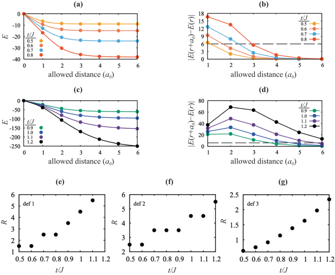

  

  a, c The lowering in the total energy, E(r), with the allowed distance (r) for a polaron to grow given each t/J parameter in our perturbation calculation. The allowed distance r is in the unit of a₀, a single unit cell length. b, d The energy correction (ΔE = ∣E(r + a₀) − E(r)∣) with the allowed distance of the electron (r), or to say, of each order of perturbation j = 2, 4, 6, 8, 10, 12. e The polaron radius changes with t/J, with the radius defined as the bound (r + a₀/2) at which E(r + a₀) − E(r) ≤ 6J. In the presence of competing low-energy physics, it is physical to define the bound of the polaron at which the additional energy gain from growing one lattice site larger ∣E(r + a₀) − E(r)∣ is insufficient to overcome the competition. f The polaron radius change with t/J, with the radius defined as the bound (r + a₀/2) at which ∣E(r + a₀) − E(r)∣/E(r)≤10%. g The polaron radius changes with t/J, with the radius defined by the full-width half maximum (FWHM) of the peak of the continuous fitting of the E(r).

  In our calculation, the farthest octahedral site that the virtual dynamic process of the carrier could reach, which is also half of the highest perturbation order, is six formula unit cells (r_k = 6). (With the perturbation calculation of different orders, we extrapolate the real trend of N_p with t/J as shown in Fig. 4c. The linear extrapolation of different t/J values is shown in Fig. 9.) We use an in-house C++ code for the perturbation calculations, with a 7 × 7 × 7 supercell size. The size of the supercell is large enough as the highest order we reach is the 12th order, which indicates 6 outward hopping steps at maximum. A periodic boundary of the system is used for the virtual hopping process. The energy of each configuration is exactly the same as in ED calculations, calculated as ${E}_{{{{\rm{config}}}}}=-{\sum }_{i,{i}^{{\prime} }}\left({J}_{i{i}^{{\prime} }}/{p}_{0}^{2}\right){{{{\bf{p}}}}}_{i}\cdot {{{{\bf{p}}}}}_{{i}^{{\prime} }}$. It is worth noting that, the carrier can hop to every neighboring site at each step as long as it returns to the original doped site after 12 hopping steps. Therefore, the carrier’s trajectory could form loops, or revisit a single site multiple times without restriction.

  Fig. 9: Convergent analysis for the average number of suppressed dipoles, N_p, against the order of perturbation, λ.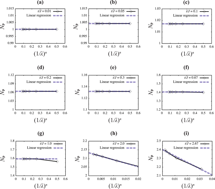

  

  N_p is plotted as a function of 1/λ at different t/J values for λ = 2, 4, 6, 8, 10, 12: (a) t/J = 0.01, n = 1; (b) t/J = 0.05, n = 1; (c) t/J = 0.1, n = 1; (d) t/J = 0.2, n = 1; (e) t/J = 0.3, n = 1; (f) t/J = 0.67, n = 1; (g) t/J = 1.0, n = 1; (h) t/J = 2.0, n = 2.5; (i) t/J = 2.67, n = 2.5.

• (iii) World-line quantum Monte Carlo (QMC): We use QMC to measure the thermal average of the FE order 〈O〉 at finite temperatures. The H_R term in Hamiltonian (Eq. (1)) is not included in order to study the quantum effect only. The FE order can be written as $\langle {{{\bf{O}}}}\rangle =\frac{1}{Z}{{{\rm{Tr}}}}({{{\bf{O}}}}\exp (-\beta H))$, where H is the Hamiltonian, β = 1/(k_BT) is the inverse temperature, and $Z={{{\rm{Tr}}}}(\exp (-\beta H))$ is the partition function. In our QMC calculation, the basis is taken as ${c}_{i}^{{\dagger} }{\prod }_{j}{a}_{j{n}_{j}}^{{\dagger} }\left\vert 0\right\rangle$. The dimension of Hilbert space is ${8}^{{L}^{3}-1}\times L$ where L is the system size. The Hamiltonian can be written in terms of H = T + H₀, where H₀ is the diagonal part and T is the non-diagonal part. Using an interaction picture, we can represent the Boltzmann factor as $\exp (-\beta H)=\exp (-\beta {H}_{0})\mathop{\sum }\nolimits_{k = 0}^{\infty }{(-1)}^{k}\int\nolimits_{0}^{\beta }\,{{{\rm{d}}}}{\tau }_{1}\int\nolimits_{0}^{{\tau }_{1}}\,{{{\rm{d}}}}{\tau }_{2}\cdots \int\nolimits_{0}^{{\tau }_{k-1}}\,{{{\rm{d}}}}{\tau }_{k}{V}_{{\tau }_{1}}^{D}{V}_{{\tau }_{2}}^{D}\cdots {V}_{{\tau }_{k}}^{D}$ where ${V}_{{\tau }_{i}}^{D}=\exp ({\tau }_{i}{H}_{0})V\exp (-{\tau }_{i}{H}_{0})$. Here we treat τ as the imaginary time and plug complete relations between each ${V}_{{\tau }_{i}}^{D}$, then 〈O〉 can be treated as a weighted average among all possible closed paths (world line) in space-time. The non-diagonal term (the kinetic part) leads to a ‘hop’ between lattice sites, thus creating a ‘kink’ on the world line. Importance sampling is done through the Metropolis algorithm. Ergodicity and detailed balance ensure the sequence of world lines converges to the desired distribution.

  We use an in-house MATLAB code for the world-line QMC calculations, with a 5 × 5 × 5 supercell under periodic boundary conditions. The supercell size used was tested by a system size scaling as shown in Fig. 10a. At every kink point, we store the imaginary time, the electron position, and the dipole configuration as matrices, and build a mapping between them. The weight of the paths and the estimator can be calculated from these matrices. In the update scheme, we generate a random kink-antikink pair at τ₁ and τ₂. Between these two time points, we propose a carrier hopping to one of the neighboring sites, randomly leaving a dipole orientation at the original site. Then, we shift the kink from τ₁ to τ₂ correspondingly. We accept these updates with certain probabilities obtained from the detailed balance. Through this scheme, the system gradually converges to its thermally equilibrated state. The calculation only converges fast at high temperatures (k_BT)/J > 0.1, below which the acceptance ratio becomes exponentially small.

  Fig. 10: Convergence check against system size in our QMC calculation and detailed T → 0 extrapolation of the resulting N_p.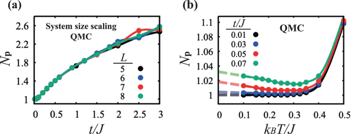

  

  a The t/J dependence of N_p at various cubic system size L³ for L = 5, 6, 7, 8 under a fixed finite temperature k_BT/J = 0.2. b Temperature dependence of N_p for different t/J parameter.

  As shown in Fig. 10b, N_p slightly decreases as T increases in the low-T range. The slight decrease in N_p is attributed to the rise in temperature, which causes the thermal distribution to suppress the impact of the virtual kinetic process by averaging out thermodynamically equilibrated Bloch states into a localized state. Figure 10b also showcases the dominance of thermal fluctuations over quantum fluctuations in the high-temperature range.

References

Li, J., Claude, J., Norena-Franco, L. E., Seok, S. I. & Wang, Q. Electrical energy storage in ferroelectric polymer nanocomposites containing surface-functionalized BaTiO3 nanoparticles. Chem. Mater. 20, 6304–6306 (2008).
Shen, Z., Wang, X., Luo, B. & Li, L. BaTiO3–BiYbO3 perovskite materials for energy storage applications. J. Mater. Chem. A 3, 18146–18153 (2015).
Lin, Y. et al. Excellent energy-storage properties achieved in BaTiO3-based lead-free relaxor ferroelectric ceramics via domain engineering on the nanoscale. ACS Appl. Mater. Interfaces 11, 36824–36830 (2019).
Fahy, S. & Merlin, R. Reversal of ferroelectric domains by ultrashort optical pulses. Phys. Rev. Lett. 73, 1122–1125 (1994).
Zenkevich, A. et al. Giant bulk photovoltaic effect in thin ferroelectric BaTiO3 films. Phys. Rev. B 90, 161409 (2014).
Sharma, S., Tomar, M., Kumar, A., Puri, N. K. & Gupta, V. Enhanced ferroelectric photovoltaic response of BiFeO3/BaTiO3 multilayered structure. J. Appl. Phys. 118, 074103 (2015).
Wang, S. et al. An unprecedented biaxial trilayered hybrid perovskite ferroelectric with directionally tunable photovoltaic effects. J. Am. Chem. Soc. 141, 7693–7697 (2019).
Arimoto, Y. & Ishiwara, H. Current status of ferroelectric random-access memory. MRS Bull. 29, 823–828 (2004).
Anderson, P. W. & Blount, E. I. Symmetry considerations on martensitic transformations: “ferroelectric” metals? Phys. Rev. Lett. 14, 217–219 (1965).
Shi, Y. et al. A ferroelectric-like structural transition in a metal. Nat. Mater. 12, 1024–1027 (2013).
Bhowal, S. & Spaldin, N. A. Polar metals: principles and prospects. Annu. Rev. Mater. Res. 53, 8.1–8.27 (2023).
Kolodiazhnyi, T., Tachibana, M., Kawaji, H., Hwang, J. & Takayama-Muromachi, E. Persistence of ferroelectricity in BaTiO3 through the insulator-metal transition. Phys. Rev. Lett. 104, 147602 (2010).
Fujioka, J. et al. Ferroelectric-like metallic state in electron doped BaTiO3. Sci. Rep. 5, 13207 (2015).
Cordero, F. et al. Probing ferroelectricity in highly conducting materials through their elastic response: Persistence of ferroelectricity in metallic BaTiO3−δ. Phys. Rev. B 99, 064106 (2019).
Zhou, W. X. et al. Artificial two-dimensional polar metal by charge transfer to a ferroelectric insulator. Commun. Phys. 2, 125 (2019).
Yang, X. et al. A doping threshold for polar metals. arXiv https://doi.org/10.48550/arXiv.2302.11721 (2023).
Wang, J. et al. Charge transport in a polar metal. npj Quant. Mater. 4, 61 (2019).
He, X. & Jin, K.-j Persistence of polar distortion with electron doping in lone-pair driven ferroelectrics. Phys. Rev. B 94, 224107 (2016).
Gu, J.-x et al. Coexistence of polar distortion and metallicity in PbTi1−xNbxO3. Phys. Rev. B 96, 165206 (2017).
Benedek, N. A. & Birol, T. ‘Ferroelectric’ metals reexamined: fundamental mechanisms and design considerations for new materials. J. Mater. Chem. C 4, 4000–4015 (2016).
Kim, T. H. et al. Polar metals by geometric design. Nature 533, 68–72 (2016).
Laurita, N. J. et al. Evidence for the weakly coupled electron mechanism in an Anderson-Blount polar metal. Nat. Commun. 10, 3217 (2019).
Lei, S. et al. Observation of quasi-two-dimensional polar domains and ferroelastic switching in a metal, Ca3Ru2O7. Nano Lett. 18, 3088–3095 (2018).
Sergienko, I. A. et al. Metallic “ferroelectricity” in the pyrochlore Cd2Re2O7. Phys. Rev. Lett. 92, 065501 (2004).
Zhang, H., Huang, W., Mei, J.-W. & Shi, X.-Q. Influences of spin-orbit coupling on Fermi surfaces and Dirac cones in ferroelectric-like polar metals. Phys. Rev. B 99, 195154 (2019).
Du, D. et al. High electrical conductivity in the epitaxial polar metals LaAuGe and LaPtSb. APL Mater. 7, 121107 (2019).
Fei, Z. et al. Ferroelectric switching of a two-dimensional metal. Nature 560, 336–339 (2018).
Sharma, P. et al. A room-temperature ferroelectric semimetal. Sci. Adv. 5, eaax5080 (2019).
Sakai, H. et al. Critical enhancement of thermopower in a chemically tuned polar semimetal MoTe2. Sci. Adv. 2, e1601378 (2016).
Wang, F. et al. Solvated electrons in solids ferroelectric large polarons in lead halide perovskites. J. Am. Chem. Soc. 143, 5–16 (2021).
Miyata, K. & Zhu, X. Y. Ferroelectric large polarons. Nat. Mater. 17, 379–381 (2018).
Kolodiazhnyi, T. Insulator-metal transition and anomalous sign reversal of the dominant charge carriers in perovskite BaTiO3−δ. Phys. Rev. B 78, 045107 (2008).
Zhu, X. Y. & Podzorov, V. Charge carriers in hybrid organic–inorganic lead halide perovskites might be protected as large polarons. J. Phys. Chem. Lett. 6, 4758–4761 (2015).
Tomioka, Y., Shirakawa, N. & Inoue, I. H. Superconductivity enhancement in polar metal regions of Sr0.95Ba0.05TiO3 and Sr0.985Ca0.015TiO3 revealed by systematic Nb doping. npj Quant. Mater. 7, 111 (2022).
Rischau, C. W. et al. A ferroelectric quantum phase transition inside the superconducting dome of Sr1−xCaxTiO3−δ. Nat. Phys. 13, 643–648 (2017).
Tangsritrakul, J. et al. Effects of iron addition on electrical properties and aging behavior of barium titanate ceramics. Ferroelectrics 383, 166–173 (2009).
Ivanchik, I. I. Spontaneous polarization screening in a single domain ferroelectric. Ferroelectrics 145, 149–161 (1993).
Härdtl, K. & Wernicke, R. Lowering the Curie temperature in reduced BaTiO3. Solid State Commun. 10, 153 – 157 (1972).
Hwang, J., Kolodiazhnyi, T., Yang, J. & Couillard, M. Doping and temperature-dependent optical properties of oxygen-reduced BaTiO3−δ. Phys. Rev. B 82, 214109 (2010).
Hlinka, J. et al. Coexistence of the phonon and relaxation soft modes in the terahertz dielectric response of tetragonal BaTiO3. Phys. Rev. Lett. 101, 167402 (2008).
Chakraborty, T. & Ray, S. Evolution of diffuse microscopic phases and magnetism in Ca, Fe co-doped BaTiO3. J. Alloys Compd 610, 271–275 (2014).
Jin, L. et al. Diffuse phase transitions and giant electrostrictive coefficients in lead-free Fe3+-doped 0.5Ba(Zr0.2Ti0.8)O3-0.5(Ba0.7Ca0.3)TiO3 ferroelectric ceramics. ACS Appl. Mater. Interfaces 8, 31109–31119 (2016).
Filippetti, A., Fiorentini, V., Ricci, F., Delugas, P. & Íñiguez, J. Prediction of a native ferroelectric metal. Nat. Commun. 7, 11211 (2016).
Puggioni, D. & Rondinelli, J. M. Designing a robustly metallic non-censtrosymmetric ruthenate oxide with large thermopower anisotropy. Nat. Commun. 5, 3432 (2014).
Michel, V. F., Esswein, T. & Spaldin, N. A. Interplay between ferroelectricity and metallicity in BaTiO3. J. Mater. Chem. C 9, 8640–8649 (2021).
Esswein, T. & Spaldin, N. A. Ferroelectric, quantum paraelectric, or paraelectric? Calculating the evolution from BaTiO3 to SrTiO3 to KTaO3 using a single-particle quantum mechanical description of the ions. Phys. Rev. Res. 4, 033020 (2022).
Klein, A., Kozii, V., Ruhman, J. & Fernandes, R. M. Theory of criticality for quantum ferroelectric metals. Phys. Rev. B 107, 165110 (2023).
Senn, M. S., Keen, D. A., Lucas, T. C. A., Hriljac, J. A. & Goodwin, A. L. Emergence of long-range order in BaTiO3 from local symmetry-breaking distortions. Phys. Rev. Lett. 116, 207602 (2016).
Wang, Y., Liu, X., Burton, J. D., Jaswal, S. S. & Tsymbal, E. Y. Ferroelectric instability under screened Coulomb interactions. Phys. Rev. Lett. 109, 247601 (2012).
Chandra, P. & Littlewood, P. B.A Landau Primer for Ferroelectrics, 69–116 (Springer Berlin Heidelberg, 2007).
Kozina, M. et al. Terahertz-driven phonon upconversion in SrTiO3. Nat. Phys. 15, 387–392 (2019).
Zhao, D. et al. Depolarization of multidomain ferroelectric materials. Nat. Commun. 10, 2547 (2019).
Jeong, I.-K. et al. Structural evolution across the insulator-metal transition in oxygen-deficient BaTiO3−δ studied using neutron total scattering and Rietveld analysis. Phys. Rev. B 84, 064125 (2011).
Stern, E. A. Character of order-disorder and displacive components in barium titanate. Phys. Rev. Lett. 93, 037601 (2004).
Berlijn, T., Lin, C.-H., Garber, W. & Ku, W. Do transition-metal substitutions dope carriers in iron-based superconductors? Phys. Rev. Lett. 108, 207003 (2012).
Wang, F. et al. Phonon signatures for polaron formation in an anharmonic semiconductor. Proc. Natl Acad. Sci. USA 119, e2122436119 (2022).
Bonn, M., Miyata, K., Hendry, E. & Zhu, X. Y. Role of dielectric drag in polaron mobility in lead halide perovskites. ACS Energy Lett. 2, 2555–2562 (2017).
Ma, J. & Wang, L.-W. Nanoscale charge localization induced by random orientations of organic molecules in hybrid perovskite CH3NH3PbI3. Nano Lett. 15, 248–253 (2015).
White, S. R. Numerical canonical transformation approach to quantum many-body problems. J. Chem. Phys. 117, 7472–7482 (2002).
Schrieffer, J. R. & Wolff, P. A. Relation between the Anderson and Kondo Hamiltonians. Phys. Rev. 149, 491–492 (1966).
Ovchinnikov, S. G. & Val’kov, V. V. Hubbard Operators in the Theory of Strongly Correlated Electrons. (Imperial College Press, 2004).
Bellaiche, L. & Íñiguez, J. Universal collaborative couplings between oxygen-octahedral rotations and antiferroelectric distortions in perovskites. Phys. Rev. B 88, 014104 (2013).
Zhong, W., Vanderbilt, D. & Rabe, K. M. First-principles theory of ferroelectric phase transitions for perovskites: The case of BaTiO3. Phys. Rev. B 52, 6301–6312 (1995).
Gu, F., Murray, E. & Tangney, P. Carrier-mediated control over the soft mode and ferroelectricity in BaTiO3. Phys. Rev. Mater. 5, 034414 (2021).
Acknowledgements
We acknowledge helpful discussions with Wei Wang, Chi-Ming Yim, Weikang Lin, and Anthony Charles Hegg. This work is supported by the National Natural Science Foundation of China (NSFC) grants #12274287 and #12042507, as well as the Innovation Program for Quantum Science and Technology (Project number: 2021ZD0301900). We also acknowledge the support from the International Postdoctoral Exchange Fellowship Program (YJ20210137) by the Office of China Postdoc Council (OCPC).
Author information
Authors and Affiliations
Contributions
W.K. and F.G. conceived the idea of the project. F.G., J.W., and Z.-J.L. developed the model through exact diagonalization, perturbation and quantum Monte Carlo approaches. F.G. performed the ED calculations and the perturbation calculations. J.W. performed the quantum Monte Carlo calculations. F.G. and W.K. analyzed the results and wrote the paper. All authors discussed the results and contributed to revising and editing the manuscript.
Corresponding author
Ethics declarations
Competing interests
The authors declare no competing interests.
Additional information
Publisher’s note Springer Nature remains neutral with regard to jurisdictional claims in published maps and institutional affiliations.
Rights and permissions
Open Access This article is licensed under a Creative Commons Attribution 4.0 International License, which permits use, sharing, adaptation, distribution and reproduction in any medium or format, as long as you give appropriate credit to the original author(s) and the source, provide a link to the Creative Commons license, and indicate if changes were made. The images or other third party material in this article are included in the article’s Creative Commons license, unless indicated otherwise in a credit line to the material. If material is not included in the article’s Creative Commons license and your intended use is not permitted by statutory regulation or exceeds the permitted use, you will need to obtain permission directly from the copyright holder. To view a copy of this license, visit http://creativecommons.org/licenses/by/4.0/.
About this article
Cite this article
Gu, F., Wang, J., Lang, ZJ. et al. Quantum fluctuation of ferroelectric order in polar metals. npj Quantum Mater. 8, 49 (2023). https://doi.org/10.1038/s41535-023-00578-3
Received:
Accepted:
Published:
DOI: https://doi.org/10.1038/s41535-023-00578-3