
Abstract
Refractory multi-principal element alloys (RMPEAs) are promising materials for high-temperature structural applications. Here, we investigate the role of short-range ordering (SRO) on dislocation glide in the MoNbTi and TaNbTi RMPEAs using a multi-scale modeling approach. Monte carlo/molecular dynamics simulations with a moment tensor potential show that MoNbTi exhibits a much greater degree of SRO than TaNbTi and the local composition has a direct effect on the unstable stacking fault energies (USFEs). From mesoscale phase-field dislocation dynamics simulations, we find that increasing SRO leads to higher mean USFEs and stress required for dislocation glide. The gliding dislocations experience significant hardening due to pinning and depinning caused by random compositional fluctuations, with higher SRO decreasing the degree of USFE dispersion and hence, amount of hardening. Finally, we show how the morphology of an expanding dislocation loop is affected by the applied stress.
Introduction
Refractory multi-principal element alloys (RMPEAs), which are composed of refractory metals in highly concentrated proportions, have garnered intense interest as promising candidate materials for high-temperature structural applications1,2. Most RMPEAs studied to date possess superior yield strengths and several RMPEAs, such as TiZrHfNbTa, TaNbTi, and HfNbTa, have reported good tensile ductility as well3,4,5,6. To accelerate design of structural RMPEAs within the vast composition space, it is necessary to understand the dislocation-based mechanisms driving their response to applied load. RMPEAs are chemically disordered at the atomic scale leading to unusual dislocation behavior. Several molecular dynamics (MD) simulations and transmission electron microscopy studies alike have pointed to stochastic glide, slip on higher-order glide planes, screw dislocation cross-kinking, and relatively low edge dislocation mobility at higher frequencies in RMPEAs than expected in pure refractories7,8,9,10,11,12.
In most studies and analyses, the chemical disorder was treated as being ideally uniformly random exhibiting no thermodynamically driven chemical short-range order (CSRO). While this may be a suitable approximation at high temperatures or for the bulk, some preferential pairing between elements in the alloy, or SRO, can be expected to manifest, especially over length scales corresponding to a dislocation. In recent years, detectable levels of SRO have been reported in both FCC MPEAs such as CoCrNi13,14,15 and CoNiV16 as well as the BCC RMPEAs such as TiZrHfNb17. Supporting calculations of SRO in MPEAs have been provided via density functional theory (DFT) and hybrid Monte Carlo (MC)/MD simulations, where temperature is used to adjust the extent and severity of SRO18,19,20,21,22,23,24,25. DFT calculations have shown that SRO in MoNbTaW RMPEA reduces the variation in the dislocation core properties, while have little effect on their core energies26. MC/MD simulations of nanocrystalline FCC and RMPEAs predict a preference for greater degrees of SRO near the grain boundaries than the interiors and overall greater strength22,27. In MD simulations of high-velocity dislocation motion, SRO tended to increase edge dislocation mobility but decrease screw dislocation mobility in RMPEA28, while the partial dislocation mobilities were decreased in an FCC MPEA22.
In this work, we seek to elucidate the extent of CSRO affects the motion of dislocations, in both mechanically under-driven and over-driven situations. We introduce a multiscale modeling approach that links a machine learning potential with quantum fidelity to hybrid MC/MD for temperature-dependent CSRO calculations at the atomic scale and ultimately to dislocation dynamics simulation of long dislocations and dislocation loops at the mesoscale. The interatomic potential presented here is a highly accurate one developed for the Mo-Ta-Nb-Ti system28,29,30,31,32. With it, two base ternary systems, MoNbTi and TaNbTi, are extracted and studied via hybrid MC/MD for CSRO at two annealing temperatures. We elected these MPEAs since experimental observations find that their equimolar forms exhibit disparate mechanical properties, with the MoNbTi being substantially greater in tensile yield strength, peak strength and strain hardening than TaNbTi. To study the effect of CSRO on the dislocation glide mechanisms, a method is developed to build statistical instantiations of large 3D crystals with spatial mapping of CSRO and associated unstable stacking fault energies (USFEs). These crystals are readily analyzable by the real-space 3D phase-field dislocation dynamics (PFDD) technique, which predicts stress-driven pathways taken by individual dislocations33,34. With the multiscale strategy, we show that SRO strengthening manifests in both MPEAs, with the average USFEs and critical stresses to initiate and sustain propagation of dislocations increasing with SRO above those for the ideal random solid solution. We introduce a figure of merit to measure SRO impact across compositions and annealing treatments and with it, reveal that CSRO strengthening contribution scales linearly with degree of SRO. The computations also reveal that gliding dislocations in subcritical conditions experience significant hardening. This glide hardening is strongly correlated to the statistical dispersion in the local USFE, and since CSRO tends to narrow the distribution in USFE, glide hardening decreases with degree CSRO. In studying dislocation loop expansion across stress regimes, a transition between jerky and smooth dislocation glide is identified and related to stress sensitivity of kink-pair nucleation rates of the screw character portions. Finally, analysis reveals that initially screw- and edge-oriented dislocations will become wavy in glide yet move via different mechanisms—kink-pair formation and migration vs. pinning/depinning. Their individual glide mechanisms do not change with composition, amount of SRO, glide distance, or subcritical or overdriven loading conditions. These computations explain why MoNbTi is the stronger one and has the greater strain hardening and forecasts that it is more amenable to SRO strengthening.
Results
Moment tensor potential
Studies of the RMPEAs here are enabled by the development of a highly accurate machine learning interatomic potential for the Mo-Ta-Nb-Ti system based on the moment tensor potential (MTP) formalism29,30,31,32. Figure 1a provides an overview of the MTP fitting procedure, which is based on a well-established workflow developed by some of the current authors in previous works27,28. To investigate the effect of composition variations on SRO and dislocation glide, the training data were carefully selected to encompass all known unary, binary, ternary and quaternary phases in the Mo-Ta-Nb-Ti system (see “Methods” section for details). Figure 1b, c show that extremely low test mean absolute errors (MAEs) were achieved for energies (4.1 meV ⋅ atom−1) and forces (0.067 eV ⋅ Å−1), comparable to that achieved previously for the NbMoTaW RMPEA27,28. The MTP also reproduces very well the DFT elastic constants for the constituent elemental systems, as shown in Supplementary Fig. 1. The shear moduli μ are 29.6 and 32.3 GPa for TaNbTi and MoNbTi, respectively, and the Young’s moduli are 82.7 and 90.7 GPa, respectively.

a Development workflow. b, c Parity plots of the MTP predicted b energies and c forces against DFT values, broken down into elemental, binary, ternary, and quaternary phases.
We also carried out several tests on the MTP’s ability to reproduce accurate thermodynamics within the Mo-Ta-Nb-Ti space. For the elements, the MTP not only successfully reproduces the correct ground state phase, but also the polymorphic energy differences to good accuracy (Supplementary Table 1). We also compared the DFT and MTP phase diagrams for the different binary systems, as shown in Supplementary Fig. 2. The MTP correctly predicts the D03 Mo3Ti and B2 MoTa intermetallics to be stable, consistent with the DFT phase diagrams. The energy above hull (Ehull) computed from DFT and MTP are also in generally good agreement (see Supplementary Table 2).
Finally, we validated the performance of the MTP in reproducing the 1/2 < 111 > edge/screw dislocation energies from DFT of elemental as well as ternary MPE systems. For the ternary MPEAs, we sampled 20 structures by randomizing the species configurations for each composition for edge/screw dislocation. As shown in Supplementary Fig. 3, a good agreement between DFT and MTP calculations for the dislocation energy is observed. The mean absolute error (MAE) is as low as 1.06 meV/atom for TaNbTi systems and 6 meV/atom for MoNbTi systems, close to the MAE of the training/test data. Also, the calculated Peierls stresses of 1/2 < 111 > screw dislocation for the BCC elemental systems using the trained MTP agree well with other reported values in the literature (Supplementary Table 3) and the qualitative trend are in line with experiments, i.e., Mo > Nb > Ta.
Chemical short-range order
To calculate the chemical SRO, bulk BCC supercells with equimolar MoNbTi and TaNbTi as well as non-equimolar ternaries with elemental ratio of 3:4:4 and 3:1:1, i.e., X4Nb3Ti4, X4Nb4Ti3, X3Nb4Ti4, X3NbTi, XNbTi3, XNb3Ti, where X = Mo or Ta, were constructed. For each composition, three levels of SRO are achieved by studying the as-constructed random solid solution (RSS) and annealing at 300 K and 1673 K using MC/MD simulations with the MTP. The SRO for the final equilibrium structures is characterized using Warren-Cowley parameters, which are defined for each pair type ij as αij = (pij − cj)/(δij − cj), where pij is the probability of having an atom type j in the nearest neighbor shell of an atom type i and cj is the concentration of type j and δij is the Kronecker delta function35. By definition, for a RSS, αij ≈ 0 and for greater degrees of SRO, the absolute value of αij increases. Figure 2 shows the Warren-Cowley parameters for the annealed RMPEAs, and Supplementary Fig. 4 plots the Warren-Cowley parameters for the equiatomic MoNbTi and TaNbTi alloys as a function of temperature in MC/MD simulations. Supplementary Figures 5–9 show the evolutions of potential energy, temperature, and SROs. For all compositions, lower annealing temperatures lead to greater levels of SRO, consistent with previous studies20,36. For the same set of elements, greater degrees of SRO can be accomplished with off-equimolar stoichiometry, i.e., the 3:1:1 and 3:4:4 compositions, than equimolar. In materials annealed at 300 K, the SRO exhibited by RMPEAs containing Mo (MoxNbyTiz) are much higher than those containing Ta (TaxNbyTiz). These two types of RMPEAs would be expected to respond differently to the same processing condition or heat treatment, with MoNbTi being much more susceptible than TaNbTi.

By definition, αij = αji for equimolar systems, which is reflected in the heatmap with a diagonal symmetric color matrix. However, for the systems with non-equimolar composition, αij ≠ αji. The color scale distinguishes between low SRO (∣αij∣ < 0.25), medium SRO (0.25 ≤ ∣αij∣ < 0.75) and high SRO (∣αij∣ ≥ 0.75).
Unstable stacking fault energy
Figure 3 plots the calculated unstable stacking fault energy (USFE) on the {110} plane, shifting along with \(< 111 >\) directions for as-constructed RSS and samples equilibrated at two different annealing temperatures. Supplementary Figure 10a–d plots the USFE distributions for all the RMPEAs with different compositions. In all cases, a higher concentration of Ti reduces the USFE. In the Mo-Nb-Ti system, greater concentrations of Mo increases the USFE, in agreement with a prior work using another interatomic potential37. On average, for the same composition, annealing at 300 K raises the USFE indicating that SRO increases USFE. To correlate the USFE with its local composition, the local composition is determined based on the composition of the first nearest neighbor planes surrounding the cleaving plane. The relationships between USFE and the local composition are plotted in Supplementary Fig. 10e. The correlations between the USFE of a plane and its local composition are consistent with those observed for average USFE of different bulk concentrations. Higher local fractions of Mo significantly increase the USFE, while higher fractions of Ta also increase the USFE but not as significantly as Mo. Higher fractions of Ti substantially decrease the USFE. The trend of USFE with local composition is consistent with the trends observed for the bulk composition as discussed above.

The values obtained from energy minimization using MTP are shown with dots. The values in the remainder of the triangles are interpolated from the calculated values and colored.
The SFE plot of different elemental systems (Supplementary Fig. 11) shows that Mo corresponds to the highest USFE of 1232 mJ/m2, and Ta and Nb have very close values of USFE of 763 and 778 mJ/m2, respectively. BCC Ti corresponds to the lowest USFE of 439 mJ/m2. Therefore, MoNbTi corresponds to higher USFE than the TaNbTi counterpart; the higher the percentage of Mo contributes to higher USFE; the higher the percentage of Ti contributes to lower USFE, as shown in Supplementary Fig. 10.
The formation energies (Eform) of binary alloys also reflect the bonding strength between different pairs in the Mo-Ta-Nb-Ti system. As shown in Supplementary Fig. 2, the Eform of Mo-Ti and Mo-Nb alloys are much more negative than the Eform of Ta-Ti and Ta-Nb alloys. The more negative the Eform, the stronger the bonding between the binary element pairs. I.e., the bonding between Mo-X is stronger than the bonding between Ta-X where X = Nb/Ti. This also explains why more percentage of Mo increases USFE significantly while Ta increases USFE less. For the Eform of the pairs including Ti, only the Mo-Ti pair corresponds to a negative Eform. Both Ti-Ta and Ti-Nb pairs have positive Eform. This indicates the bonding strength of Ta and Nb with Ti is weak. Therefore, explaining the more percentage of Ti decreases the USFE.
We can also explain the trend from the perspective of BCC lattice bond length and electronegativity, as shown in Supplementary Table 4. The order of bond length is Ta > Nb > Ti > Mo. The order of electronegativity is Mo > Nb > Ti > Ta. The bond length of Mo is significantly smaller than the rest of the elements. The electronegativity of Mo is remarkably larger than the rest of the elements. These two factors produce stronger bonding for Mo with the rest of the elements. Therefore, the presence of Mo increases the USFE.
The SRO of different pairs from 300 K also reflects the bonding preference in MPEAs. As shown in Fig. 2, for equimolar systems, the SRO of the Mo-Ti pair is negative (attractive interaction), while the Ta-Ti pair is positive (repulsive interaction). The SROs of Mo-Nb and Ta-Nb are both negative, but the value for the Mo-Nb pair (−0.26) is much more negative than that of the Ta-Nb pair (−0.01). Consequently, the MoNbTi corresponds to higher USFE compared to the TaNbTi.
The driving forces for the differences in the SRO can be attributed to pairwise interactions, as explained from the perspective of binary formation energy, bond length, and electronegativity.
Phase-field framework
PFDD was employed to simulate the behavior of dislocations in both alloys. While atomistic studies of, for example, Peierls stresses in MPEAs are informative for characterizing the range of stresses for very short dislocation segments, as shown in Supplementary Figure 12, they do not give insight into the behavior of long dislocations over realistic timescales. As a mesoscale model, PFDD sacrifices atomic-scale fidelity in exchange for information about the morphologies, mechanisms, and glide resistances of long dislocations and loops under stress. Through PFDD, emergent properties of dislocations propagating through the chemically disordered glide plane can be uncovered. Such findings would not be accessible through a Peierls stress calculation of a short, straight segment.
In PFDD, the dislocation is represented through scalar order parameters ϕ, from which a total energy is determined and minimized (see Methods34,). We use three order parameters, ϕ1, ϕ2, and ϕ3, to represent the dislocation habit plane and two cross slip planes38. All inputs into PFDD are physical, such as the elastic constants, lattice parameters, and USFE, and are obtained from the MTP calculations in the preceding sections. In an MPEA, the resistance to dislocation glide is not homogeneous within the material due to variations in local composition7,8,39,40,41. A dislocation will only be affected by the type and arrangement of atomic elements within a radius of a few Burgers vectors42. As such, at any position and point in time, the dislocation only samples a small nanoscale region of the crystal with a local composition differing from that of the bulk. In PFDD, the local composition of every nanometer region is associated with its corresponding USFE. We account for these spatial variation in composition by creating a crystal with spatial variation USFE, simulating the variable resistance to dislocation glide43,44. The elastic stiffness tensor is assumed to be constant throughout the cell. Atomistic calculations of the stiffness of various non-equiatomic compositions of the MPEAs show that elastic constants do not change appreciably with composition (Supplementary Table 5).
To generate position-dependent USFE crystals for MoNbTi and TaNbTi, random lattices with target SRO levels were created using the OTIS (order through informed swapping) method45. OTIS uses a statistical swapping procedure and is based on binary alloy swapping method adapted from Gehlen et al.46 (see the “Methods” section). Each lattice point in a random lattice is then assigned a local composition, which is defined as the composition of the atom and its neighbors up to the 5th nearest neighbor within two adjacent (110) planes. The 5th nearest neighbor was chosen based on atomistic simulations of solute-dislocation interaction energies42, and only atoms within the two (110) planes that would be sheared by a dislocation were considered. A local USFE value was then determined using the USFE-composition maps in Fig. 3. A linear interpolation scheme is used to estimate the USFE for compositions not directly calculated. We verified that the scheme produces USFE values with less than 5% error. In total, 420 lattices containing several million atoms were created for each level of SRO for both alloys, with examples shown in Supplementary Fig. 13.
To quantify SRO based on the Warren-Cowley parameters, we introduce ω as the Euclidean norm of the three like-pair Warren-Cowley parameters \(\omega =\sqrt{{\alpha }_{11}^{2}+{\alpha }_{22}^{2}+{\alpha }_{33}^{2}}\) as a single figure of merit (FOM) ω that can be used to compare the relative extent of SRO in an equimolar alloy. With it, we find that the mean USFE scales directly with ω (Supplementary Fig. 14a). The MoNbTi alloy reaches a higher ω for the same set of annealing treatment due to the preference for Mo-Ti and Mo-Nb bonds. The coefficient of variation (CV) in USFE tends to decrease with ω, a consequence of the reduction in random atomic pairings (Supplementary Fig. 14b).
Dislocation glide mechanisms
We first study the role of SRO on the glide behavior of initially straight edge or screw dislocations. Due to the randomness in underlying fault energies, twenty independent realizations are performed for each alloy and each level of SRO. To study critical behavior, the applied shear stress is gradually increased in increments of 0.001μ until the dislocation glides and is held constant until it fully arrests.
Figure 4 shows snapshots in time of edge dislocation glide. When the stress is initially applied and raised, the dislocation remains straight. Once the applied stress exceeds the first threshold, the edge dislocation becomes slightly wavy, as small portions of the dislocation line bow out into low USFE regions and are held back at the higher USFE regions. The stress must be increased further for the dislocation to glide, and small bowed out segments of the dislocation will glide independently through the lower USFE regions, dragging the neighboring (non-edge) segments through the higher USFE regions. The dislocation arrests several times during the simulation, each time requiring the stress to be raised to restart glide. The arrested dislocation morphologies are wavy, unlike the original pure edge orientation. The stop/start behavior leads to glide plane hardening, a continual increase in applied stress with increasing plastic strain, as seen in the stress-strain curve in Fig. 4. This is in contrast to PFDD simulations of pure metals, in which dislocations gliding have a single critical stress and remain straight during glide.

a–d and e–h show edge and screw glide, respectively, in a TaNbTi sample at 300K SRO. i–l and m–p show edge and screw glide, respectively, in a MoNbTi sample at 300K SRO.
Screw dislocation glide proceeds in a different manner from edge dislocation glide. As the stress increases, the dislocation remains completely straight with pure screw character until a kink-pair only a few Burgers vectors wide is nucleated into a low USFE region. Kink-pairs form naturally when a screw dislocation segment advances by one Burgers vector in a location where the local applied stress exceeds the local resistance. Unlike the variable wavy bow out in the edge dislocation, these kink-pairs always have a height of just 1b, and the kinks will usually, but not always, glide along the length of the screw dislocation to advance the full dislocation line forward. Like the edge dislocations, the screw dislocations may become arrested under stress, but unlike the edge dislocations, the arrested dislocation morphologies are nearly straight, apart from a few metastable kinks, recovering the original pure screw orientation. The start/stop mechanism of glide of the screw dislocation also leads to glide plane hardening, although at a lower level than edge dislocation glide plane hardening.
Dislocation core structures
The different dislocation glide mechanisms can be related to differences in their core structures. The zero-stress, relaxed dislocation core structures, represented through the PFDD order parameters, are shown for MoNbTi in Fig. 5. An equivalent figure for TaNbTi can be found in the Supplementary Figure 15. Two MoNbTi core structures for both screw and edge dislocations are chosen: one in an “easy” region with a lower critical stress and one in a “hard” region with a higher critical stress. For comparison, core structures in a material with the pure Mo and pure Nb USFE are also shown. The elastic constants for all of these structures are the same, so any differences are attributable to USFE alone. The local dislocation core structure changes as the dislocation glides due to the changing local UFSE.

The first and second rows show dislocation in pure Mo and pure Nb, respectively, using the MoNbTi elastic constants. The third and fourth rows show dislocation segments with low and high critical stresses, respectively. The core width within the habit plane is annotated.
As is well-known for BCC materials and observed in prior PFDD simulations38, screw dislocation cores spread onto the three equivalent 110-type slip planes while edge dislocation cores remain planar. The non-planar structure of screw dislocations is responsible for the increased glide stresses and the predominance of kink-pair nucleation glide mechanisms. The width w of the dislocation core in the (110) habit plane is estimated by measuring the distance between ϕ1 = 0.05 and ϕ1 = 0.95, using a linear interpolation between grid points as necessary. Higher local USFE values produce narrower dislocations. Dislocations in pure Mo have the narrowest cores, while Ti-rich regions of MoNbTi have the widest cores. Wider dislocation cores are associated with lower Peierls stresses47, thus explaining the link between lower USFE and lower critical stresses.
Dislocation glide stresses
Figure 6a plots the stresses to initiate glide σi and the final stresses for runaway glide σf of edge and screw dislocations based on twenty independent initializations. Regardless of SRO, both σi and σf for the TaNbTi alloy are lower than those for the MoNbTi alloy. From Fig. 6b, we find that mean glide resistance across the plane scales directly with the average USFE across the plane. Thus, changes in USFE caused by SRO have a direct influence on the stress to initiate and propagate dislocations, as seen in Fig. 6c. The higher the ω, the higher the USFE is increased relative to the RSS case, which translates directly to increased glide resistance for both screw and edge dislocations.

a The mean critical stress for dislocations in each of the alloys. The critical stresses for MoNbTi and TaNbTi are normalized by their respective shear moduli μ. The error bars show the resolution of the simulation, 0.001 μ. b The mean initial critical stress vs the mean USFE for each alloy. c The mean initial critical stress relative to the mean initial critical stress for RSS alloy vs the extent of SRO, represented by the SRO FOM. The black × represents the RSS case. d The hardening, represented by the difference in final and initial critical stresses, vs the coefficient of variation of USFE. e The hardening relative to the hardening for the RSS alloy vs the extent of SRO.
We also find that the hardening in glide resistance is related to the degree of dispersion of the USFE values in the glide plane as opposed to the mean. In Fig. 6d, we analyze the role of composition and its fluctuations by adopting the fractional increase from σi to σf as a measure of glide-plane hardening. While screw dislocations do not experience significant hardening, the hardening of edge dislocations scales directly with the USFE CV for both alloys. The strikingly linear relationship, even when considering both alloys, implies that it transcends composition. Thus, apparent differences in the hardening seen in these alloys can be explained. Compared to TaNbTi, MoNbTi achieves, on average, greater hardening in the ideal random case and lower hardening in the highest ω case.
Further, while hardening for both screw and edge dislocations increase as the USFE CV increases, the edge dislocations experience greater hardening than the screw dislocations for the same statistically sampled glide plane length (Fig. 6d). The edge dislocations glide by depinning of the segments at the relatively harder regions, segments which have reoriented to non-edge character due to bow out. Continued glide, therefore, relies on overcoming those local regions of higher resistance. Encountering a region ahead of the dislocation of even greater resistance than in the wake more likely occur when the dispersion in USFE is greater. The screw dislocation moves by producing short and narrow atomic advances of screw-oriented segments, i.e., kink-pairs, in the weaker regions and relying on the long advances of easier-to-move edge segments along the length of the dislocation. Those local domains of higher resistance that are more likely encountered when the dispersion in USFE is higher, can be easily overcome by migrating edge dislocations. By virtue of their differing glide mechanisms, edge dislocations experience greater sensitivity to the dispersion in USFE and hence greater hardening than screw dislocations.
Figure 6e examines the influence of ω on hardening. It reveals that the role of SRO on hardening corresponds to the extent to which SRO affects the CV in USFE. As increased ω tends to narrow the dispersion in USFE across the glide plane, it reduces glide-plane hardening. Since the TaNbTi alloy achieves lower ω than MoNbTi for the same annealing treatment, hardening, like its strength, is weakly affected by SRO compared to MoNbTi.
Effect of chemical fluctuations on glide mobility
Next, we study the effect of chemical fluctuations on screw/edge glide mobility by examining loop expansion on the (110) slip plane at constant stress. For given applied stress, thirty dislocation loop expansion simulations are conducted representing different locations in a given alloy and SRO. We find that for all cases, the anisotropy in screw/edge behavior reduces with increases applied stress. At low stresses, the difference in screw/edge behavior is large, causing the loop to expand into an oblong shape (Fig. 7a–c). The edge segments move continuously, constantly changing their wavy appearance. The screw dislocations advance very slowly, nucleating only a few kink-pairs at a time and recovering the nearly straight orientation with each advancement. As the applied stress increases, both screw and edge velocities increase and their ratio decreases towards unity. The loop expands more isotropically, almost FCC-like (Fig. 7d–f). Figure 7f shows the loop at both low and high stress overlaid together. The two loops have similar widths (103b and 101b, respectively) but different heights (38b and 51b, respectively), demonstrating that higher stresses decrease the loop aspect ratio. The screw dislocation has clearly changed its mode of glide, as a result of a higher kink-pair nucleation rate. The screw portions move continuously and adopt a wavy appearance, superficially much like the edge dislocations. Wavy screw glide, however, occurs as many kink-pairs nucleate simultaneously along the same dislocation. Newly advanced portions can nucleate further kink pairs, causing different portions of the dislocations to advance at different rates.

The initial loop shape is shown by the dotted lines in a and d. When a lower stress is applied, the screw dislocation nucleates kink-pairs infrequently, causing jerky dislocation glide and remaining largely pure screw. At higher applied stresses, the screw dislocation nucleates many kink-pairs at once resulting in smoother glide and a wavy morphology. The final loop from c is reproduced by the dashed line in f to highlight the difference in aspect ratio between the two loops.
We separate the two extremes of screw dislocation behavior into “jerky” glide at low stresses and “smooth” glide at high stresses. To link the transition between jerky and smooth dislocation the rate of kink-pair nucleation, we calculate the waiting time between kink-pair nucleation events for all simulations. The waiting times from all thirty instantiations of loops are combined into a single distribution for a given alloy and applied stress, and the means are plotted in Fig. 8. Over 22,000 and 52,000 total waiting times were recorded for TaNbTi and MoNbTi, respectively, and each individual distribution contains at least 200 values. For both TaNbTi and MoNbTi, higher levels of SRO correspond to longer average waiting times and thus more jerky dislocation glide at all applied stresses. Normalizing the applied stresses by the average σi for screw glide, the three distinct SRO curves collapse into one. Thus, the critical stress to transition from jerky to smooth scales with Peierls strength or with static strength. SRO affects the transition stress in dynamic glide indirectly via its strengthening effect on static glide resistance.

The error bars show the standard error. The transition between jerky and smooth screw dislocation glide is determined by the applied stress relative to the dislocation critical stress.
Discussion
There are limited experimental measurements of the mechanical properties of TaNbTi and MoNbTi. The tensile yield stresses have been reported as 620 and 950 MPa for TaNbTi and MoNbTi, respectively8,48,49, which are consistent with the dislocation dynamics predictions of higher glide stresses for MoNbTi. The ultimate tensile strengths are 683 and 1500 MPa, respectively, so MoNbTi exhibits significant strain hardening while TaNbTi does not. Our simulations show higher hardening in MoNbTi than TaNbTi due to the increased coefficient of variation in USFE. The dislocation dynamics simulations also revealed that the amount of dislocation hardening is decreased by the presence of SRO, especially for MoNbTi. As edge dislocations undergo more hardening than screw dislocations, we predict the differences in macro-scale strain hardening in these alloys are largely controlled by edge dislocation behavior.
From the Warren-Cowley parameter calculations, it is clear that MoNbTi has a higher propensity for SRO and will be more affected by processing conditions. There has been interest in tuning the SRO parameters through heat treatment, although experimentally, this is difficult to achieve15. Findings indicate that MoNbTi is a better candidate for exploring SRO strengthening than TaNbTi since SRO promotes two relatively stronger Mo-Nb and Mo-Ti bonds. However, the relative increases in the average dislocation glide resistance due to SRO amount to less than 20% even in the most extreme cases, so large changes in the mechanical properties must be accompanied by changes in the chemical composition, not SRO alone.
Via MD simulations, a few studies have shown SRO-enhanced dislocation glide resistance15,28,50 and one study on CoFeNiTi alloy reported a slight SRO softening51. Strengthening or softening was related to the formation of immobile dislocation segments via cross slip. Here, we demonstrate SRO strengthening in dislocation glide without cross slip. While the current dislocation model permits cross slip38, it was not observed in the present calculations since the influence of thermal fluctuations is not taken into account. Including temperature would undoubtedly increase the chance for cross-slip or cross-kinking, adding another mechanism for SRO strengthening.
Methods
Training data generation
The moment tensor potential (MTP) formalism, which has been shown to yield a good balance between accuracy and computational cost31, was utilized in this work. Details about the MTP formalism can be found in previous works52,53,54.
A comprehensive training dataset is essential to developing a robust MTP. In this work, the training data include the elemental, binary, ternary, and quaternary chemical systems. In addition to ground state bulk structures, distorted bulk structures, surfaces, stacking faults, and grain boundaries were also included to improve the accuracy for potential in calculating planar defects. The detailed structure generation for each system is provided as follows.
-
1.
Elemental systems (BCC Mo, Ta, Nb, Ti, and HCP Ti)
-
(a)
Ground state structures for the elements, i.e., BCC Mo, Ta, Nb, and HCP Ti, plus BCC Ti;
-
(b)
Distorted structures constructed by applying strains of −10% to 10% at 1% intervals to the bulk conventional cell for BCC Mo, Ta, Nb, Ti, and HCP Ti. Detailed can be found in ref. 55;
-
(c)
Surface structures of elemental metals obtained from the Crystalium database56;
-
(d)
Grain boundary structures of elemental metals obtained from grain boundary database57;
-
(e)
Snapshots from NVT ab initio molecular dynamics (AIMD) simulations of the bulk 3 × 3 × 3 supercell for BCC and 4 × 4 × 2 supercell for HCP Ti at room temperature, medium temperature (below melting point), high temperature (above melting point). In addition, snapshots were also obtained from NVT AIMD simulations at room temperature at 90% and 110% of the equilibrium 0 K volume. Forty snapshots were extracted from each AIMD simulation at intervals of 0.1 ps; 100 snapshots from high-temperature (above melting point) NPT simulations are also included for each element.
-
(a)
-
2.
Binary systems (Mo-Ta, Mo-Nb, Mo-Ti, Ta-Nb, Ta-Ti, Nb-Ti)
-
(a)
Solid solution structures constructed by partial substitution of 2 × 2 × 2 bulk supercells of one element with the other element. Compositions of the form AxB1−x were generated with x ranging from 0 at% to 100 at% at intervals of 6.25 at%.
-
(a)
-
3.
Ternary and quaternary systems (Mo-Ta-Nb, Mo-Ta-Ti, Mo-Nb-Ti, Ta-Nb-Ti, Mo-Ta-Nb-Ti)
-
(a)
Special quasi-random structures (SQS)58 generated with ATAT59 using a 4 × 4 × 4 BCC supercell.
-
(b)
Snapshots from NVT AIMD simulations of the Mo-Nb-Ti SQS structure at 300, 1000, and 3000 K with addition of 100 snapshots structures from NPT AIMD simulations at 3200 K. Snapshots from NPT AIMD simulations of Ta-Nb-Ti SQS at 300, 900, 1500, 2400, and 3000 K.
-
(c)
Surface structures56, stacking fault structures samples37,60 for Mo-Nb-Ti, Ta-Nb-Ti, and Mo-Ta-Nb-Ti systems.
-
(d)
Stacking fault structures obtained from refs. 37,60 for ternary and quaternary systems.
-
(a)
With each alloying percentage, we performed structure relaxations for all symmetrically distinct binary solid solution structures. We include both unrelaxed and relaxed structures in the data set. For ternary and quaternary systems, we considered the permutation of the elements in SQS structures. We also included structures from each ionic relaxation step of permutated SQS structure samples in the data set.
All the training data were generated using the same convergence criteria used in our previous work27. The database includes 17,210 static calculations as training data and 1660 as test dataset.
Atomistic simulations
All the atomistic simulations using MTP were performed using LAMMPS61. The simulation cells are oriented along the [112], [\(\bar{1}\)10] and [11\(\bar{1}\)] cubic crystollagraphic directions, which are the main directions of interest for slip in the BCC system. A supercell of dimensions of ~ 48 Å × 46 Å × 46 Å with 5760 atoms was used.
-
Hybrid MC/MD simulations within the isothermal-isobaric (NPT) ensemble were carried out for different compositions (equimolar, element ratio of 3:3:4 and 1:1:3) for ternary alloys MoxNbyTiz and TaxNbyTiz. The supercells were randomly initialized based on the desired stoichiometry, i.e., a RSS. The simulations were then carried out at 300 K and 1673 K to obtain the equilibrium configurations with different degrees of short-range order. Periodic boundary conditions were applied to all three directions. The Metropolis algorithm was used to attempt a swap between species type 1 and 2, species type 1 and type 3, and species type 2 and type 3 at every time step. The MD time step was set to 2 fs. The evolutions of energy, temperature, and SROs of different pairs for various compositions from MC/MD calculations can be found in Supplementary Figs. 5–9. After the converged configurations were reached through MC/MD, all the systems were then relaxed at 300 K using NPT MD. The structures with different composition and SROs were used for stacking fault energy calculations with energy minimization at 0 K.
-
USFE calculations. The conjugate gradient algorithm was used to perform stacking fault structure relaxation and energy minimization. The force components within (110) plane are set to zero. The direction perpendicular to (110) plane was allowed to fully relax. The schematic in Fig. 9 shows the procedures of sampling the stacking faults with different local compositions. From the equilibrated bulk MPEA structures, different stacking faults were sampled by changing the cutting layer positions along (110) plane, and shifting the right chunk of bulk along with \(< 111 >\) direction. The composition of two atomic layers along (110) plane at the cutting position is used to represent the local composition of the sampled stacking fault.
Fig. 9: The procedures of sampling the stacking faults with different local compositions. 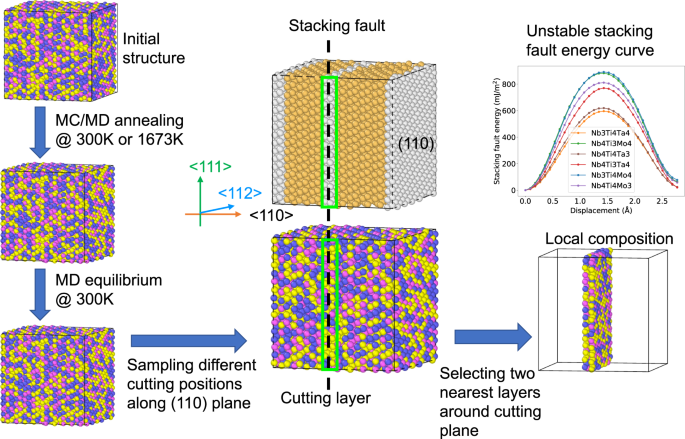
The initial structure is a re-oriented supercell with x, y, and z directions along the [112], [\(\hbox{-}{\bar{1}}10\)], and [\(11{\hbox{-}{\bar{1}}}\)] directions, respectively, with a random solid solution. After the MC/MD annealing at 300K and 1673K and MD equilibrium at 300K, different cutting positions are sampled along the (110) plane for different compositions. The top right panel shows one sample of the stacking fault energy curve for different compositions. The first nearest neighbor atomic layers of the cutting plane are selected as the local composition of the stacking fault.

Creation of random lattices
Our method to generate the random lattices with SRO is based on the method of Gehlen and Cohen, who used a swapping procedure to create binary FCC lattices with SRO46. We extend this method to multi-component alloys and only consider SRO in the first nearest neighbor (NN) shell. First, a BCC lattice of the desired shape is created, and each lattice point is randomly assigned an element type such that the overall composition is equilimolar. The total number of each bond type (e.g. Nb-Nb, Nb-Ti, etc.) is calculated. Using the Warren-Cowley SRO parameters, a goal number of each type of bond can be determined. Atoms are then swapped until the actual number of each bond type is equal to the goal. At each iteration, two lattice points with unlike element types are randomly selected. If swapping these atoms will move the bond numbers closer to the goal, the atoms are swapped. If not, the swap is rejected and a new pair of lattice points is selected. To increase the likelihood that a swap is accepted, the atoms selected for a swap are not chosen from the entire lattice but instead from a subset of atoms with desirable neighborhoods. For each element type, the expected number of each type of element in its NN shell can be predicted. When randomly selecting atoms to swap, we only choose from lattice points that do not have the expected atoms in their NN shell. For example, if the current number of i-j bonds is higher than the goal number of i-j bonds, we can select an i-atom with more j-atoms than expected in its NN shell to swap with a j-atom with more i-atoms than expected in its NN shell. Using this smarter swapping method for an MoNbTi lattice with the 300 K SRO parameters increases the acceptance percentage from 15% to 63% and decreases the running time by more than a factor of 10.
Once the lattice has the desired SRO parameters, we assign each point a composition based on the type of the atom and up to its 5th nearest neighbor within two adjacent (110) planes for a total of 31 atoms. This composition is identified on the linearly interopolated USFE plots in Fig. 3 in order to assign each lattice point a USFE value.
Phase-field dislocation dynamics
PFDD is a mesoscale model used to study dislocation glide through crystals. The full details of the PFDD method are given elsewhere34,43,62. PFDD tracks the dislocation configuration through scalar order parameters ϕα(r) where α corresponds to a slip system with Burgers vector bα and plane normal nα. When ϕα(r) = 0 or 1, point r is unslipped or slipped by a full dislocation of type α, respectively. Intermediate values of ϕα(r) at the interface between slipped and unslipped regions correspond to dislocations. The order parameters are used to calculate a total system energy ψ(ϕ(r)), which is then minimized by the Ginzburg-Landau equation to evolve the dislocations.
where t is time and m0 is a dislocation mobility coefficient. There are three energy contributions to the total energy: the lattice energy ψlatt(ϕ(r)), the elastic energy ψelas(ϕ(r)), and the external energy ψext(ϕ(r)):
The elastic energy accounts for the elastic strain in the crystal and is given by
where cijkl is the elastic stiffness tensor and \({\epsilon }_{ij}^{e}\) is the elastic strain which can be calculated from the order parameters63. The external energy accounts for the work done by an applied stress field and is given by
where \({\sigma }_{ij}^{{{{\rm{app}}}}}\) is the applied stress state.
The final energy term, lattice energy represents the energy to break bonds at the dislocation core, and its form is specific to the material being studied. Because dislocations in BCC crystals have compact cores, a simple sinusoidal approximation is used64
where γusf is the USFE, d is the slip plane interplanar spacing, and N is the number of slip systems.
In each PFDD simulation, three order parameters are used to represent three different slip systems, each with a Burgers vector \(\frac{a}{2}[\bar{1}11]\). The slip planes are (110), \((01\bar{1})\), and (101). Allowing glide on three different slip planes makes cross slip possible and gives the distinct screw-edge differences seen in BCC materials38. A BCC primitive cell is used to define the lattice grid points with primitive vectors \({{{{\bf{p}}}}}_{1}=\frac{b}{\sqrt{3}}[11\bar{1}]\), \({{{{\bf{p}}}}}_{2}=\frac{b}{\sqrt{3}}[\bar{1}11]\), and \({{{{\bf{p}}}}}_{3}=\frac{b}{\sqrt{3}}[1\bar{1}1]\). In each simulation, the first order parameter is set to 0 or 1 depending on the initial dislocation configuration to create a dislocation on the (110) plane. All other order parameters are initially zero. For the screw dislocation dipole simulations, a 128b × 362b × 136b simulation cell is used, and the dislocations are initially 362b long and separated by 32b. For the edge dislocation dipole simulations, a 128b × 128b × 384b simulation cell is used, and the dislocations are also initially 362b long and separated by 32b. In the dislocation loop simulations, a 128b × 128b × 128b cell is used and the initial loop radius is 16b.
Data availability
To ensure the reproducibility and use of the models developed in this paper, all the training and test data (structures, energies, force, etc.) are available at figshare https://doi.org/10.6084/m9.figshare.19247931as a downloadable zipped BSON file.
The trained quaternary potential for MoTaNbTi is available in the GitHub repository of the open-source Materials Machine Learning (maml) package at https://github.com/materialsvirtuallab/maml/tree/master/mvl_models/pes.
Code availability
The codes used to train the potential are available at https://github.com/materialsvirtuallab/mamland https://gitlab.com/ashapeev/interface-lammps-mlip-2.
All atomistic simulations were executed using open-source software LAMMPS. The dislocation structures used in atomistic calculations are generated via Atomsk65 https://atomsk.univ-lille.fr/tutorial_Al_edge.php. The PFDD code used in this study and the associated documentation is available under an open-source license at https://github.com/lanl/Phase-Field-Dislocation-Dynamics-PFDD. All the other codes that support the findings of this study are available from Hui Zheng (email: huz071@eng.ucsd.edu) upon request.
References
Senkov, O. & Semiatin, S. Microstructure and properties of a refractory high-entropy alloy after cold working. J. Alloy. Compd. 649, 1110–1123 (2015).
Sheikh, S. et al. Alloy design for intrinsically ductile refractory high-entropy alloys. J. Appl. Phys. 120, 164902 (2016).
Dirras, G. et al. Elastic and plastic properties of as-cast equimolar TiHfZrTaNb high-entropy alloy. Mater. Sci. Eng.: A 654, 30–38 (2016).
George, E. P., Raabe, D. & Ritchie, R. O. High-entropy alloys. Nat. Rev. Mater. 4, 515–534 (2019).
George, E., Curtin, W. & Tasan, C. High entropy alloys: A focused review of mechanical properties and deformation mechanisms. Acta Mater. 188, 435–474 (2020).
Wang, S.-P., Ma, E. & Xu, J. New ternary equi-atomic refractory medium-entropy alloys with tensile ductility: Hafnium versus titanium into NbTa-based solution. Intermetallics 107, 15–23 (2019).
Rao, S. et al. Modeling solution hardening in BCC refractory complex concentrated alloys: NbTiZr, Nb1.5TiZr0.5 and Nb0.5TiZr1.5. Acta Mater. 168, 222–236 (2019).
Wang, F. et al. Multiplicity of dislocation pathways in a refractory multiprincipal element alloy. Science 370, 95–101 (2020).
Chen, B. et al. Unusual activated processes controlling dislocation motion in body-centered-cubic high-entropy alloys. Proc. Natl Acad. Sci. USA 117, 16199–16206 (2020).
Lee, C. et al. Strength can be controlled by edge dislocations in refractory high-entropy alloys. Nat. Commun. 12, 5474 (2021).
Rao, S., Woodward, C., Akdim, B., Senkov, O. & Miracle, D. Theory of solid solution strengthening of BCC Chemically Complex Alloys. Acta Mater. 209, 116758 (2021).
Xu, S., Jian, W.-R., Su, Y. & Beyerlein, I. J. Line-length-dependent dislocation glide in refractory multi-principal element alloys. Appl. Phys. Lett. 120, 061901 (2022).
Zhang, R. et al. Short-range order and its impact on the CrCoNi medium-entropy alloy. Nature 581, 283–287 (2020).
Zhang, F. X. et al. Local structure and short-range order in a NiCoCr solid solution alloy. Phys. Rev. Lett. 118, 205501 (2017).
Ding, J., Yu, Q., Asta, M. & Ritchie, R. O. Tunable stacking fault energies by tailoring local chemical order in CrCoNi medium-entropy alloys. Proc. Natl Acad. Sci. USA 115, 8919–8924 (2018).
Chen, X. et al. Direct observation of chemical short-range order in a medium-entropy alloy. Nature 592, 712–716 (2021).
Wang, S. D. et al. Chemical short-range ordering and its strengthening effect in refractory high-entropy alloys. Phys. Rev. B 103, 104107 (2021).
Singh, P., Smirnov, A. V. & Johnson, D. D. Atomic short-range order and incipient long-range order in high-entropy alloys. Phys. Rev. B 91, 224204 (2015).
Wróbel, J. S., Nguyen-Manh, D., Lavrentiev, M. Y., Muzyk, M. & Dudarev, S. L. Phase stability of ternary fcc and bcc Fe-Cr-Ni alloys. Phys. Rev. B 91, 024108 (2015).
Fernández-Caballero, A., Wróbel, J. S., Mummery, P. M. & Nguyen-Manh, D. Short-range order in high entropy alloys: theoretical formulation and application to Mo-Nb-Ta-V-W system. J. Phase Equilib. Diffus. 38, 391–403 (2017).
Ma, Y. et al. Chemical short-range orders and the induced structural transition in high-entropy alloys. Scr. Mater. 144, 64–68 (2018).
Jian, W.-R. et al. Effects of lattice distortion and chemical short-range order on the mechanisms of deformation in medium entropy alloy CoCrNi. Acta Mater. 199, 352–369 (2020).
Zhao, S. Local ordering tendency in body-centered cubic (BCC) multi-principal element alloys. J. Phase Equilib. Diffus. 42, 578–591 (2021).
Jian, W.-R., Wang, L., Bi, W., Xu, S. & Beyerlein, I. J. Role of local chemical fluctuations in the melting of medium entropy alloy CoCrNi. Appl. Phys. Lett. 119, 121904 (2021).
Xie, Z. et al. Role of local chemical fluctuations in the shock dynamics of medium entropy alloy CoCrNi. Acta Mater. 221, 117380 (2021).
Yin, S., Ding, J., Asta, M. & Ritchie, R. O. Ab initio modeling of the energy landscape for screw dislocations in body-centered cubic high-entropy alloys. npj Comput. Mater. 6, 110 (2020).
Li, X.-G., Chen, C., Zheng, H., Zuo, Y. & Ong, S. P. Complex strengthening mechanisms in the NbMoTaW multi-principal element alloy. npj Comput. Mater. 6, 70 (2020).
Yin, S. et al. Atomistic simulations of dislocation mobility in refractory high-entropy alloys and the effect of chemical short-range order. Nat. Commun. 12, 4873 (2021).
Chen, C. et al. Accurate force field for molybdenum by machine learning large materials data. Phys. Rev. Mater. 1, 043603 (2017).
Li, X.-G. et al. Quantum-accurate spectral neighbor analysis potential models for Ni-Mo binary alloys and fcc metals. Phys. Rev. B 98, 094104 (2018).
Zuo, Y. et al. Performance and cost assessment of machine learning interatomic potentials. J. Phys. Chem. A 124, 731–745 (2020).
Qi, J. et al. Bridging the gap between simulated and experimental ionic conductivities in lithium superionic conductors. Mater. Today Phys. 21, 100463 (2021).
Xu, S. Recent progress in the phase-field dislocation dynamics method. Comput. Mater. Sci. 210, 111419 (2022).
Beyerlein, I. J. & Hunter, A. Understanding dislocation mechanics at the mesoscale using phase field dislocation dynamics. Philos. Trans. R. Soc. A: Math. Phys. Eng. Sci. 374, 20150166 (2016).
Cowley, J. M. An approximate theory of order in alloys. Phys. Rev. 77, 669–675 (1950).
Kostiuchenko, T., Körmann, F., Neugebauer, J. & Shapeev, A. Impact of lattice relaxations on phase transitions in a high-entropy alloy studied by machine-learning potentials. npj Comput. Mater. 5, 55 (2019).
Xu, S., Hwang, E., Jian, W.-R., Su, Y. & Beyerlein, I. J. Atomistic calculations of the generalized stacking fault energies in two refractory multi-principal element alloys. Intermetallics 124, 106844 (2020).
Fey, L. T. W., Hunter, A. & Beyerlein, I. J. Phase-field dislocation modeling of cross-slip. J. Mater. Sci. 57, 10585–10599 (2022).
Maresca, F. & Curtin, W. A. Theory of screw dislocation strengthening in random BCC alloys from dilute to “High-Entropy” alloys. Acta Mater. 182, 144–162 (2020).
Xu, S., Su, Y., Jian, W.-R. & Beyerlein, I. J. Local slip resistances in equal-molar MoNbTi multi-principal element alloy. Acta Mater. 202, 68–79 (2021).
Romero, R. A., Xu, S., Jian, W.-R., Beyerlein, I. J. & Ramana, C. Atomistic simulations of the local slip resistances in four refractory multi-principal element alloys. Int. J. Plasticity 149, 103157 (2022).
Ghafarollahi, A., Maresca, F. & Curtin, W. Solute/screw dislocation interaction energy parameter for strengthening in bcc dilute to high entropy alloys. Model. Simul. Mater. Sci. Eng. 27, 085011 (2019).
Smith, L. T., Su, Y., Xu, S., Hunter, A. & Beyerlein, I. J. The effect of local chemical ordering on Frank-Read source activation in a refractory multi-principal element alloy. Int. J. Plasticity 134, 102850 (2020).
Fey, L. T. W., Xu, S., Su, Y., Hunter, A. & Beyerlein, I. J. Transitions in the morphology and critical stresses of gliding dislocations in multiprincipal element alloys. Phys. Rev. Mater. 6, 013605 (2022).
Fey, L. T. W. & Beyerlein, I. J. Random generation of lattice structures with short-range order. Integr. Mater. Manuf. Innov. 11, 382–390 (2022).
Gehlen, P. C. & Cohen, J. B. Computer simulation of the structure associated with local order in alloys. Phys. Rev. 139, A844–A855 (1965).
Joos, B. & Duesbery, M. The peierls stress of dislocations: an analytic formula. Phys. Rev. Lett. 78, 266 (1997).
Zýka, J. et al. Microstructure and room temperature mechanical properties of different 3 and 4 element medium entropy alloys from HfNbTaTiZr system. Entropy 21, 114 (2019).
Senkov, O., Miracle, D. & Rao, S. Correlations to improve room temperature ductility of refractory complex concentrated alloys. Mater. Sci. Eng. A 820, 141512 (2021).
Li, Q.-J., Sheng, H. & Ma, E. Strengthening in multi-principal element alloys with local-chemical-order roughened dislocation pathways. Nat. Commun. 10, 3563 (2019).
Antillon, E., Woodward, C., Rao, S. & Akdim, B. Chemical short range order strengthening in BCC complex concentrated alloys. Acta Mater. 215, 117012 (2021).
Shapeev, A. V. Moment tensor potentials: a class of systematically improvable interatomic potentials. Multiscale Model. Simul. 14, 1153–1173 (2016).
Gubaev, K., Podryabinkin, E. V., Hart, G. L. & Shapeev, A. V. Accelerating high-throughput searches for new alloys with active learning of interatomic potentials. Comput. Mater. Sci. 156, 148–156 (2019).
Podryabinkin, E. V., Tikhonov, E. V., Shapeev, A. V. & Oganov, A. R. Accelerating crystal structure prediction by machine-learning interatomic potentials with active learning. Phys. Rev. B 99, 064114 (2019).
de Jong, M. et al. Charting the complete elastic properties of inorganic crystalline compounds. Sci. Data 2, 150009 (2015).
Tran, R. et al. Surface energies of elemental crystals. Sci. Data 3, 160080 (2016).
Zheng, H. et al. Grain boundary properties of elemental metals. Acta Mater. 186, 40–49 (2020).
Zunger, A., Wei, S.-H., Ferreira, L. G. & Bernard, J. E. Special quasirandom structures. Phys. Rev. Lett. 65, 353–356 (1990).
van de Walle, A., Asta, M. & Ceder, G. The alloy theoretic automated toolkit: a user guide. Calphad 26, 539–553 (2002).
Hu, Y.-J., Sundar, A., Ogata, S. & Qi, L. Screening of generalized stacking fault energies, surface energies and intrinsic ductile potency of refractory multicomponent alloys. Acta Mater. 210, 116800 (2021).
Plimpton, S. Fast parallel algorithms for short-range molecular dynamics. J. Comput. Phys. 117, 1–19 (1995).
Xu, S., Su, Y., Smith, L. T. W. & Beyerlein, I. J. Frank-Read source operation in six body-centered cubic refractory metals. J. Mech. Phys. Solids 141, 104017 (2020).
Xu, S., Su, Y. & Beyerlein, I. J. Modeling dislocations with arbitrary character angle in face-centered cubic transition metals using the phase-field dislocation dynamics method with full anisotropic elasticity. Mech. Mater. 139, 103200 (2019).
Peng, X., Mathew, N., Beyerlein, I. J., Dayal, K. & Hunter, A. A 3D phase field dislocation dynamics model for body-centered cubic crystals. Comput. Mater. Sci. 171, 109217 (2020).
Hirel, P. Atomsk: a tool for manipulating and converting atomic data files. Comput. Phys. Commun. 197, 212–219 (2015).
Acknowledgements
L.T.W.F. acknowledges support from the Department of Energy National Nuclear Security Administration Stewardship Science Graduate Fellowship, which is provided under cooperative agreement number DE-NA0003960. SX and IJB gratefully acknowledge support from the Office of Naval Research under contract ONR BRC Grant N00014-21-1-2536. Use was made of computational facilities purchased with funds from the National Science Foundation (CNS-1725797) and administered by the Center for Scientific Computing (CSC). The CSC is supported by the California NanoSystems Institute and the Materials Research Science and Engineering Center (MRSEC; NSF DMR 1720256) at UC Santa Barbara. H.Z., X.G.L., C.C., and S.P.O. acknowledge support from the Office of Naval Research under Grant number N00014-18-1-2392 and computational resources provided by the University of California, San Diego, and the Extreme Science and Engineering Discovery Environment (XSEDE) supported by the National Science Foundation under grant no. ACI-1548562. LQ acknowledges support from the National Science Foundation (NSF) under award DMR-1847837 and computational resources provided by Extreme Science and Engineering Discovery Environment (XSEDE) Stampede2 at the TACC through allocation TG-DMR190035.
Author information
Authors and Affiliations
Contributions
H.Z. and X.G.L. generated the DFT training data. H.Z. trained the ML potential and performed the atomistic calculations. L.T.W.F. designed and performed the PFDD calculations. Y.J.H., L.Q., and S.X. contributed the DFT training data of stacking faults for ternary and quaternary systems. L.T.W.F. and H.Z. wrote the manuscript with input from all authors. C.C., S.X., I.J.B., and S.P.O. supervised the project. I.J.B. and S.P.O. designed the project. H.Z., L.T.W.F., and X.G.L. contributed equally.
Corresponding authors
Ethics declarations
Competing interests
The authors declare no competing interests.
Additional information
Publisher’s note Springer Nature remains neutral with regard to jurisdictional claims in published maps and institutional affiliations.
Supplementary information
Rights and permissions
Open Access This article is licensed under a Creative Commons Attribution 4.0 International License, which permits use, sharing, adaptation, distribution and reproduction in any medium or format, as long as you give appropriate credit to the original author(s) and the source, provide a link to the Creative Commons license, and indicate if changes were made. The images or other third party material in this article are included in the article’s Creative Commons license, unless indicated otherwise in a credit line to the material. If material is not included in the article’s Creative Commons license and your intended use is not permitted by statutory regulation or exceeds the permitted use, you will need to obtain permission directly from the copyright holder. To view a copy of this license, visit http://creativecommons.org/licenses/by/4.0/.
About this article

Cite this article
Zheng, H., Fey, L.T.W., Li, XG. et al. Multi-scale investigation of short-range order and dislocation glide in MoNbTi and TaNbTi multi-principal element alloys. npj Comput Mater 9, 89 (2023). https://doi.org/10.1038/s41524-023-01046-z
Received:
Accepted:
Published:
DOI: https://doi.org/10.1038/s41524-023-01046-z
This article is cited by
-
Random Generation of Lattice Structures with Short-Range Order
Integrating Materials and Manufacturing Innovation (2022)
