Self-supervised optimization of random material microstructures in the small-data regime

Abstract

While the forward and backward modeling of the process-structure-property chain has received a lot of attention from the materials’ community, fewer efforts have taken into consideration uncertainties. Those arise from a multitude of sources and their quantification and integration in the inversion process are essential in meeting the materials design objectives. The first contribution of this paper is a flexible, fully probabilistic formulation of materials’ optimization problems that accounts for the uncertainty in the process-structure and structure-property linkages and enables the identification of optimal, high-dimensional, process parameters. We employ a probabilistic, data-driven surrogate for the structure-property link which expedites computations and enables handling of non-differential objectives. We couple this with a problem-tailored active learning strategy, i.e., a self-supervised selection of training data, which significantly improves accuracy while reducing the number of expensive model simulations. We demonstrate its efficacy in optimizing the mechanical and thermal properties of two-phase, random media but envision that its applicability encompasses a wide variety of microstructure-sensitive design problems.

Introduction

Inverting the process-structure-property (PSP) relationships represents a grand challenge in materials science as it holds the potential of expediting the development of new materials with superior performance^1,2. While significant progress has been made in the forward and backward modeling of the process-structure and structure-property linkages and in capturing the nonlinear and multiscale processes involved³, much fewer efforts have attempted to integrate uncertainties which are an indispensable component of materials’ analysis and design^4,5. Uncertainties can arise since: (a) process variables do not fully determine the resulting microstructure but rather a probability distribution on microstructures⁶, (b) noise and incompleteness are characteristic of experimental data that are used to capture process-structure (most often) and structure-property relations⁷, (c) models employed for the process-structure or structure-property links are often stochastic and there is uncertainty in their parameters or form, especially in multiscale formulations⁸, and (d) model compression and dimension reduction employed in order to gain efficiency unavoidably lead to some loss of information which in turn gives rise to predictive uncertainty⁹. This randomness should be incorporated, not only in the forward modeling of the PSP chain, but in the optimization objectives and the inverse-design tasks as well.

(Back-)propagating uncertainty through complex and potentially multiscale models poses significant computational difficulties¹⁰. Data-based surrogates can alleviate these as long as the number of training data, i.e., the number of solutions of the complex models they would substitute, is kept small. In this small-data setting additional uncertainty arises due to the predictive inaccuracy of the surrogate. Quantifying it can not only lead to more accurate estimates but also guide the acquisition of additional experimental/simulation data.

We note that problem formulations based on Bayesian Optimization^11,12,13 account for uncertainty in the objective solely due to the imprecision of the surrogate and not due to the aleatoric, stochastic variability of the underlying microstructure. In the context of optimization/design problems in particular, a globally-accurate surrogate would be redundant. It would suffice to have a surrogate that can reliably drive the optimization process to the vicinity of the optimum (or optima) and can sufficiently resolve this (those) in order to identify the optimal control parameters. Since the location of the optima is, a priori, unknown, adaptive strategies, in which the training of the surrogate and the optimization are coupled, would be necessary.

We emphasize that unlike successful efforts e.g., in topology optimization¹⁴ or general heterogeneous media¹⁵ which find a single, optimal microstructure maximizing some property-based objective, our goal is more ambitious but also more consistent with the physical reality. We attempt to find the value of the processing variables that gives rise to the optimal distribution of microstructures (Fig. 1). To address the computational problem arising from the presence of uncertainties, we recast the stochastic optimization as a probabilistic inference task and employ approximate inference techniques based on Stochastic Variational Inference (SVI¹⁶).

Fig. 1: Conceptual overview.

Given stochastic process-structure and structure-property links, we identify the process parameters φ* which maximize the expected utility ${{\mathbb{E}}}_{p\left({{{\boldsymbol{x}}}}| \varphi \right)}\left[u\left({{{\boldsymbol{\kappa }}}}\right)\right]$ (Illustration based on the specific case $u\left({{{\boldsymbol{\kappa }}}}\right)={{\mathbb{I}}}_{{{{\mathcal{K}}}}}\left({{{\boldsymbol{\kappa }}}}\right)$ and $p\left({{{\boldsymbol{\kappa }}}}| {{{\boldsymbol{x}}}}\right)=\delta \left({{{\boldsymbol{\kappa }}}}-{{{\boldsymbol{\kappa }}}}\left({{{\boldsymbol{x}}}}\right)\right)$). (Micro)Structures x arise from a stochastic process through the density $p\left({{{\boldsymbol{x}}}}| \varphi \right)$ which depends on the process parameters φ. A data-driven surrogate is employed to predict properties ${\boldsymbol{\kappa }}$ which introduces additional uncertainty.

In terms of the stochastic formulation of the problem, our work most closely resembles that of¹⁷ where they seek to identify a probability density on microstructural features which would yield a target probability density on the corresponding properties. While this poses a challenging optimization problem, producing a probability density on microstructural features does not provide unambiguous design guidelines. In contrast, we operate on (and average over) the whole distribution of microstructures and consider a much wider range of design objectives. In¹⁸ random microstructures were employed but their macroscopic properties were insensitive to their random variability (due to scale-separation) and low-dimensional parametrizations of the two-point correlation function were optimized using gradient-free tools. In a similar fashion, in^19,20 analytic, linear models were employed which, given small and Gaussian uncertainties on the macroscopic properties, find the underlying orientation distribution function (ODF) of the crystalline microstructure. In^21,22, averaged macroscopic properties (ignoring the effects of crystal size and shape) were computed with respect to the ODF of the polycrystalline microstructure and on the basis of their targeted values, the corresponding ODF is found. While data-based surrogates were also employed, the problem formulation did not attempt to quantify the effect of microstructural uncertainties.

In terms of surrogate development, in this work we focus on the microstructure-property link and consider random, binary microstructures, the distribution of which depends on some processing-related parameters. We develop active learning strategies that are tailored to the optimization objectives. The latter can account for the potential stochasticity of the material properties (as well as the predictive uncertainty of the surrogate), i.e., we enable the solution of optimization-under-uncertainty problems.

Results & discussion

It is advisable that the readers familiarize themselves with the mathematical entities defined in the "Methods" section in order to better appreciate the results presented in this section which contains two applications of the methodological framework, for (O1)- and (O2)-type formulations of the inversion of the PSP chain (see "Methods"). We first elaborate on the specific choices for the process parameters φ, the random microstructures x and their properties ${\boldsymbol{\kappa }}$ as well as the associated PSP links.

Process φ - Microstructure x

In all numerical illustrations we consider statistically homogeneous, binary (two-phase) microstructures which upon spatial discretization (on a uniform, two-dimensional N_p × N_p grid with N_p = 64) are represented by a vector x ∈ {0, 1}⁴⁰⁹⁶. The binary microstructures are modeled by means of a thresholded zero-mean, unit-variance Gaussian field^23,24. If the vector x_g denotes the discretized version of the latter (on the same grid), then the value at each pixel i is given by x_i = H(x_g,i − x₀) where H( ⋅ ) denotes the Heaviside function and x₀ the cutoff threshold, which determines the volume fractions of the resulting binary field. We parameterize the spectral density function (SDF) of the underlying Gaussian field (i.e., the Fourier transform of its autocovariance) with φ, using a combination of radial basis functions (RBFs—see Supplementary Notes) which automatically ensures the non-negativity of the resulting SDF. The constraint of unit variance is enforced using a softmax transformation. The density p(x∣φ) implicitly defined above affords great flexibility in the resulting binary microstructures (as can be seen in the ensuing illustrations) which increases as the dimension of φ does. Figure 1 illustrates how different values of the process parameters φ can lead to profound changes in the microstructures (and correspondingly, their effective physical properties ${\boldsymbol{\kappa }}$). While the parameters φ selected do not have explicit physical meaning, they can be linked to actual processing variables given appropriate data. Naturally, not all binary media can be represented by this model and a more flexible p(x∣φ), potentially learned from actual process-structure data, could be employed with small modifications in the overall algorithm^25,26,27.

Microstructure x - Properties ${\boldsymbol{\kappa }}$

In this study we consider a two-dimensional, representative volume element (RVE) Ω_RVE = [0, 1]² and assume each of the two phases are isotropic, linear elastic in terms of their mechanical response and are characterized by isotropic, linear conductivity tensors in terms of their thermal response. We denote with ${\mathbb{C}}$ the fourth-order elasticity tensor and with a the second order conductivity tensor which are also binary (tensor) fields. The vector ${\boldsymbol{\kappa }}$ consists of various combinations of macroscopic, effective (apparent), mechanical or thermal properties of the RVE which we denote by ${{\mathbb{C}}}^{{{\mbox{eff}}}}$ and a^eff, respectively. The effective properties for each microstructure occupying Ω_RVE were computed using finite element simulations and Hill’s averaging theorem^28,29 (further details are provided in the Supplementary Notes). We assumed a contrast ratio of 50 in the properties of the two phases, i.e., E₁/E₀ = 50 (where E₀, E₁ are the elastic moduli of phases 0 and 1, as well as Poisson’s ratio ν = 0.3 for both phases) and a₁/a₀ = 50 (where a₀, a₁ are the conductivities of phases 0 and 1). In the following plots, phase 1 is always shown with white and phase 0 with black. We note that the dependence of effective properties on (low-dimensional) microstructural features (analogous to φ) has been considered, in e.g.^30,31, but the random variability in these properties has been ignored either by considering very large RVEs or by averaging over several of them. We emphasize finally that the framework proposed can accommodate any high-fidelity model for the structure-property link as this is merely used as a generator for the training data ${{{\mathcal{D}}}}$.

Case 1: Target domain of multi-physics properties (O1)

In the following we will demonstrate the performance of the proposed formulation in an (O1)-type stochastic optimization problem (see “Methods”), with regards to both thermal as well as mechanical properties. In addition, we will provide a systematic and quantitative assessment of the benefits of the active learning strategy proposed (as compared to randomized data generation).

We consider a combination of mechanical and thermal properties of interest, namely [Eq. 1]:

$${\kappa }_{1}={[{{{{\boldsymbol{a}}}}}^{{{\mbox{eff}}}}]}_{11},\qquad {\kappa }_{2}=\frac{1}{2}\left({[{{\mathbb{C}}}^{{{\mbox{eff}}}}]}_{1111}+{[{{\mathbb{C}}}^{{{\mbox{eff}}}}]}_{2222}\right)$$

(1)

i.e., ${{{\boldsymbol{\kappa }}}}\in {{\mathbb{R}}}_{+}^{2}$, and define the target domain [Eq. 2]:

$${{{\mathcal{K}}}}=\left[8.5,\,11.0\right]\times \left[6.75,\,9.0\right]$$

(2)

The utility function $u({{{\boldsymbol{\kappa }}}})={{\mathbb{I}}}_{{{{\mathcal{K}}}}}\left({{{\boldsymbol{\kappa }}}}\right)$ is the (non-differentiable) indicator function of ${{{\mathcal{K}}}}\subset {{\mathbb{R}}}_{+}^{2}$ which implies that the objective of the optimization (type (O1)—see Fig. 2a) is to find the φ that maximizes the probability that the resulting microstructures have properties ${\boldsymbol{\kappa }}$ that lie in ${{{\mathcal{K}}}}$. The two-phase microstructures have volume fraction 0.5 and the parameters $\varphi \in {{\mathbb{R}}}^{100}$ as well as p(x∣φ) were defined as discussed in the beginning of this section.

Fig. 2: Illustration of various materials design objectives.

Different optimization objectives with respect to the density $p\left({{{\boldsymbol{\kappa }}}}| \varphi \right)$ that expresses the likelihood of property values ${\boldsymbol{\kappa }}$ for given processing conditions φ. We illustrate the following cases: (a) we seek to maximize the probability that the material properties ${\boldsymbol{\kappa }}$ fall within a target domain ${{{\mathcal{K}}}}$. (b) We seek to minimize the mean deviation of the properties ${\boldsymbol{\kappa }}$ from a target value ${\boldsymbol{\kappa }}_{target}$. (c) we seek to minimize the deviation between $p\left({{{\boldsymbol{\kappa }}}}| \varphi \right)$ and a target probability density ${p}_{target}\left({{{\boldsymbol{\kappa }}}}\right)$ on the material properties.

With regards to the adaptive learning strategy (appearing as the outer loop in Algorithm (1) in “Methods”), we note that the initial training dataset ${{{{\mathcal{D}}}}}^{(0)}$ consists of N₀ = 2048 data pairs which are generated via ancestral sampling, i.e., we randomly draw samples φ from ${{{\mathcal{N}}}}({{{\boldsymbol{0}}}},{{{\boldsymbol{I}}}})$ and conditionally on each φ⁽ⁿ⁾ we sample p(x∣φ⁽ⁿ⁾) to generate a microstructure (the choice $\varphi \sim {{{\mathcal{N}}}}({{{\boldsymbol{0}}}},{{{\boldsymbol{I}}}})$ is not arbitrary, as—given the adopted parametrization—it envelopes all possible SDFs). In each data acquisition step l, N_pool = 4096 candidates were generated and a subset of N_add = 1024 of those was selected based on the acquisition function. We note that N_add (as well as N₀) defines a trade-off between information acquisition and computational cost. Hence the size of the dataset increased by 1024 data pairs at each iteration l, with L = 4 data augmentation steps performed in total.

The optimal process parameters at each data acquisition step are denoted as ${\varphi }_{{{{\mathcal{M}}}},{{{{\mathcal{D}}}}}^{(l)}}^{* }$, with the subscript indicating the dependence on the surrogate model ${{{\mathcal{M}}}}$ and the dataset ${{{{\mathcal{D}}}}}^{(l)}$ on which it has been trained. Once the algorithm has converged to its final estimate of the process parameters after L data acquisition steps, i.e., ${\varphi }_{{{{\mathcal{M}}}},{{{{\mathcal{D}}}}}^{(L)}}^{* }$, we can assess ${\varphi }_{{{{\mathcal{M}}}},{{{{\mathcal{D}}}}}^{(L)}}^{* }$ by obtaining a reference estimate of the expected utility $U({\varphi }_{{{{\mathcal{M}}}},{{{{\mathcal{D}}}}}^{(L)}}^{* })=Pr({{{\boldsymbol{\kappa }}}}\in {{{\mathcal{K}}}}| {\varphi }_{{{{\mathcal{M}}}},{{{{\mathcal{D}}}}}^{(L)}}^{* })$ using Monte Carlo, i.e., by sampling microstructures ${{{\boldsymbol{x}}}} \sim p({{{\boldsymbol{x}}}}| {\varphi }_{{{{\mathcal{M}}}},{{{{\mathcal{D}}}}}^{(L)}}^{* })$, and running the high-fidelity model instead of the inexpensive surrogate. In this manner we can also compare the optimization results obtained with active learning with those obtained by using randomized training data ${{{\mathcal{D}}}}$ (i.e., without adaptive learning). We argue that the former has a competitive advantage, if for the same total number N of datapoints we can achieve a higher score in terms of our materials’ design objective $Pr\left({{{\boldsymbol{\kappa }}}}\in {{{\mathcal{K}}}}| {\varphi }^{* }\right)$. As the optimization objective ${{{\mathcal{F}}}}$ is non-convex and the optimization algorithm itself non-deterministic, generally the optimal process parameters φ* identified can vary across different runs (non-determinancy arises from the randomized generation of the data, the stochastic initialization of the neural network, as well as the randomized initial guess of ${\varphi }^{(0)} \sim {{{\mathcal{N}}}}\left({{{\boldsymbol{0}}}},{{{\boldsymbol{I}}}}\right)$) . For this reason the optimization problem is solved several times (with different randomized initializations) and we report on the aggregate performance of active learning vs. randomized data generation (baseline).

In the following we discuss the results obtained and displayed in Figs. 3, 4, 5 and 6.

• In Fig. 3 we depict sample microstructures drawn from p(x∣φ) for two values of φ, i.e., for the initial guess φ⁽⁰⁾ (Fig. 3a) and for optimal process parameters ${\varphi }_{{{{\mathcal{M}}}},{{{{\mathcal{D}}}}}^{(L)}}^{* }$ (Fig. 3b). While the optimized microstructures as shown in Fig. 3b remain random, one observes that the connectivity of phase 1 (stiffer) is increased as compared to the microstructures shown in Fig. 3a. The diagonal, connected paths of the lesser conducting phase (black) effectively block heat conduction in the horizontal direction. This is also reflected in the effective properties reported underneath each image. The value of the objective, i.e., the probability that properties ${\boldsymbol{\kappa }}$ reside in ${{{\mathcal{K}}}}$, is ≈ 0.65 for the optimal microstructures (Fig. 3b), as opposed to ≈ 0.14 for the microstructures shown in Fig. 3b (see also Fig. 4a and c).

• Figure 4 provides insight into the optimization algorithm proposed by looking at the process-property density p(${\boldsymbol{\kappa }}$∣φ) for various φ values. We note that this density is implicitly defined by propagating the randomness in the microstructures (quantified by p(x∣φ)) through the high-fidelity model that predicts the properties of interest. Based on the Monte Carlo estimates depicted in Fig. 4, one observes that the density p(${\boldsymbol{\kappa }}$∣φ) only minimally touches the target domain ${{{\mathcal{K}}}}$ for initial process parameters φ⁽⁰⁾ (Fig. 4a) and gradually moves closer to ${{{\mathcal{K}}}}$ as the iterations proceed, with the optimization informed by the surrogate trained on the initial batch of data ${{{{\mathcal{D}}}}}^{(0)}$ (Fig. 4b). The incorporation of additional training data by means of the adaptive learning scheme enables the surrogate to resolve the details in the structure-property map with sufficient detail to eventually identify process parameters such that the density p(${\boldsymbol{\kappa }}$∣φ) maximally overlaps (in comparison) with the target domain ${{{\mathcal{K}}}}$ (Fig. 4c).

• In Fig. 5a we illustrate the performance advantage gained by the active learning approach proposed over the baseline. To this end, we compare the values of the objective function, i.e., $Pr({{{\boldsymbol{\kappa }}}}\in {{{\mathcal{K}}}}| {\varphi }_{{{{\mathcal{M}}}},{{{\mathcal{D}}}}}^{* })$ achieved for datasets ${{{\mathcal{D}}}}$ of equal size, with the dataset being either generated randomly (baseline), or constructed based on our active learning approach. Evidently, the latter was able to achieve a better material design at comparably significantly lower numerical cost (as measured by the number of evaluations of the high-fidelity model of the S-P link). We observe that while the addition of more training data generally leads to more accurate surrogates, when this is done without regard to the optimization objectives (red line), then it does not necessarily lead to higher values of the objective function. In Fig. 5b we provide further insight as to why the adaptive data acquisition was able to outperform a randomized approach. To this end we consider the impact of adaptive learning on the model belief for one of the effective properties ${\boldsymbol{\kappa }}$, i.e., we compare the model-based belief $p({\kappa }_{1}| {\varphi }_{{{{\mathcal{M}}}},{{{{\mathcal{D}}}}}^{(4)}}^{* },{{{{\mathcal{D}}}}}^{(0)})$ of the surrogate conditional on ${{{{\mathcal{D}}}}}^{(0)}$ against a reference density obtained using Monte Carlo (black line). We can see that a model only informed by ${{{{\mathcal{D}}}}}^{(0)}$ (red line) identifies an incorrect density and as such fails to converge to the optimal process parameters. The active learning approach (blue line) was able to correct the initially erroneous model belief and as a result performs better in the optimization task.

• In Fig. 6a we illustrate the evolution of the ELBO during the inner-loop iterations of the proposed VB-EM algorithm (see Algorithm (1) in “Methods”). Finally, in Fig. 6b we depict the evolution of the maximum of the objective identified at various data acquisition steps l of the proposed active learning scheme in a single, indicative run (in contrast to Fig. 5 where results over multiple runs are summarized). As it can be seen, the targeted data enrichment enables the surrogate to resolve details in the structure-property map and identify higher-performing processing parameters φ.

Fig. 3: Case 1: Optimal random microstructures.

(a) Samples of microstructures drawn from p(x∣φ) for the initial guess φ⁽⁰⁾ of processing variables. (b) Samples of microstructures drawn from p(x∣φ) for the optimal value ${\varphi }_{{{{\mathcal{M}}}},{{{{\mathcal{D}}}}}^{(L)}}^{* }$ of processing variables which maximize the probability that the corresponding material properties will fall in the target domain ${{{\mathcal{K}}}}=\left[8.5,\,11.0\right]\times \left[6.75,\,9.0\right]$ (Eq. (2)). Underneath each microstructure, the thermal ${\kappa }_{1}$ and mechanical ${\kappa }_{2}$ properties of interest (Eq. (1)) are reported.

Fig. 4: Case 1: Evolution of the process-property density during optimization.

The actual process-property density $p\left({{{\boldsymbol{\kappa }}}}| \varphi \right)$ was estimated using 1024 Monte Carlo samples making use of the high-fidelity structure-property model (see Supplementary Notes), and for the following three values of the process parameters φ: (a) for the initial guess φ⁽⁰⁾, (b) for the optimal φ as obtained using the initial training dataset ${{{{\mathcal{D}}}}}^{(0)}$ and without adaptive learning, (c) for the optimal φ obtained with the augmented training dataset ${{{{\mathcal{D}}}}}^{(4)}$ identified by the active learning scheme proposed. The target domain ${{{\mathcal{K}}}}$ (Eq. (2)) is drawn with a green rectangle and the colorbar indicates the value of the density $p\left({{{\boldsymbol{\kappa }}}}| \varphi \right)$.

Fig. 5: Case 1: Assessment of active learning approach.

(a) The probability we seek to maximize with respect to φ, i.e., $Pr\left({{{\boldsymbol{\kappa }}}}\in {{{\mathcal{K}}}}| \varphi \right)$ is plotted as a function of the size N of the training dataset (i.e., the number of simulations of the high-fidelity model). Based on 80 independent runs of the optimization algorithm, we plot the median value (with dots) and the 50% probability quantiles (with error bars). The red lines correspond to the results obtained without adaptive learning and the blue with adaptive learning. (b) For the the optimal ${\varphi }_{{{{\mathcal{M}}}},{{{{\mathcal{D}}}}}^{(4)}}^{* }$ identified using active learning, we compare the actual process-property density $p({{{\kappa }}}_{1}| \varphi )$ (black line—estimated with 1024 Monte Carlo samples and the high-fidelity model) with the one predicted by the surrogate trained only on the initial dataset ${{{{\mathcal{D}}}}}^{(0)}$ (red line) and with the one predicted by the surrogate trained on the augmented dataset ${{{{\mathcal{D}}}}}^{(4)}$ (blue line).

Fig. 6: Case 1: Convergence characteristics of the optimization algorithm.

We illustrate for a single optimization run (a) the evolution of the ELBO ${{{\mathcal{F}}}}$ as a function of the iteration number in the inner loop and for l = 0 (outer loop—see Algorithm (1)). (b) Evolution of the probability we seek to maximize $Pr({{{\boldsymbol{\kappa }}}}\in {{{\mathcal{K}}}}| \varphi )$ (estimated with 1024 Monte Carlo samples and the high-fidelity model) for the optimal values ${\varphi }_{{{{\mathcal{M}}}},{{{{\mathcal{D}}}}}^{(l)}}^{* }$ identified by the algorithm at various data acquisition steps l (outer loop in Algorithm (1)).

Case 2: Target density of properties (O2)

In this second numerical illustration, we investigate the performance of the proposed methodological framework for an (O2)-type optimization problem (Eq. (7)) where we seek to identify the processing parameters φ that lead to a property density $p\left({{{\boldsymbol{\kappa }}}}| \varphi \right)$ that is closest to a prescribed target ${p}_{target}\left({{{\boldsymbol{\kappa }}}}\right)$. In particular, we considered the following two properties [Eq. 3]

$${\kappa }_{1}={\left[{{{{\boldsymbol{a}}}}}^{{{\mbox{eff}}}}\right]}_{11}\qquad \qquad \qquad {\kappa }_{2}={\left[{{{{\boldsymbol{a}}}}}^{{{\mbox{eff}}}}\right]}_{22}$$

(3)

i.e., ${{{\boldsymbol{\kappa }}}}\in {{\mathbb{R}}}^{2}$ and a target density [Eq. 4]:

$${p}_{target}\left({{{\boldsymbol{\kappa }}}}\right)={{{\mathcal{N}}}}\left(\hat{{{{\boldsymbol{\mu }}}}},{{{\hat{\boldsymbol{{{\Sigma }}}}}}}\right)$$

(4)

with ${{{\hat{\boldsymbol{\mu }}}}}={\left[20.5,3.5\right]}^{T}$ and ${\hat{{{\Sigma }}}}_{11}=0.60$, ${\hat{{{\Sigma }}}}_{22}=0.01,{\hat{{{\Sigma }}}}_{12}=-0.03$ (depicted with green iso-probability lines in Fig. 8). These values were selected to promote anisotropic behavior, i.e., the targeted microstructures should have a large effective conductivity in the first spatial dimension and simultaneously be (relatively) insulating in the second spatial dimension. The characteristics of the active learning procedure (outer loop in Algorithm (1) in “Methods”) remain identical, with the only difference that ${{{{\mathcal{D}}}}}^{(0)}$ now comprises N₀ = 4096 datapoints, with N_add = 1024 datapoints (out of 4096 candidates) added in each of the L = 6 data-enrichment steps. We used S = 20 samples from ${p}_{target}\left({{{\boldsymbol{\kappa }}}}\right)$ to approximate the objective (see Eq. (9)).

We discuss the results obtained based on Figs. 7 and 8:

• In Fig. 7 we showcase sample microstructures drawn from $p\left({{{\boldsymbol{x}}}}| \varphi \right)$ both for the initial guess φ⁽⁰⁾ (Fig. 7a, b) as well as for the optimal process parameters ${\varphi }_{{{{\mathcal{M}}}},{{{{\mathcal{D}}}}}^{(L)}}^{* }$ identified by the optimization algorithm using the active learning approach (Fig. 7c, d). The examples shown in Fig. 7a, b correspond to volume fraction 0.5 whereas the examples shown in Fig. 7b, d correspond to volume fraction 0.3 (of the more conducting, white phase, a₁) . As one would expect, we observe that the optimal family of microstructures identified (determined by ${\varphi }_{{{{\mathcal{M}}}},{{{{\mathcal{D}}}}}^{(L)}}^{* }$) exhibit connected paths of the more conductive phase (white) along the horizontal direction. The connected paths of the lesser conducting phase (black) are also aligned in the horizontal direction so as to reduce the effective conductivity along the vertical direction. The optimal microstructures therefore exhibit a marked anistropy and funnel heat through pipe-like structures of high-conductivity material in the horizontal direction. This is also reflected in the indicative property values reported under each frame.

• Finally, Fig. 8 assesses the advantage of the active learning strategy advocated for this problem. In particular, we plot the evolution of the process-structure density $p\left({{{\boldsymbol{\kappa }}}}| \varphi \right)$ in relation to the target ${p}_{target}\left({{{\boldsymbol{\kappa }}}}\right)$ (depicted with green iso-probability lines) at different stages of the optimization (initial-intermediate-converged). Using the optimal process parameters φ identified at each of these stages, we see that the optimization scheme without active learning (Fig. 8a–d) results in a density that is quite far from the target. In contrast, the optimization algorithm with active learning (Fig. 8e–h) is able to identify a φ which brings the $p\left({{{\boldsymbol{\kappa }}}}| \varphi \right)$ very close to the target distribution ${p}_{target}\left({{{\boldsymbol{\kappa }}}}\right)$. The validity of this result is assessed in (Fig. 8i–l) where the actual $p\left({{{\boldsymbol{\kappa }}}}| \varphi \right)$ (estimated with Monte Carlo and the high-fidelity model) is depicted for the φ values identified by the active learning approach (Fig. 8e–h). We observe a very close agreement which reinforces previous evidence on the advantages of the active learning strategy advocated.

Fig. 7: Case 2: Optimal random microstructures.

(a), (b) Samples of microstructures drawn from p(x∣φ) for the initial guess φ⁽⁰⁾ of processing variables. (c), (d) Samples of microstructures drawn from $p\left({{{\boldsymbol{\kappa }}}}| \varphi \right)$ for the optimal value ${\varphi }_{{{{\mathcal{M}}}},{{{{\mathcal{D}}}}}^{(6)}}^{* }$ of the processing variables which minimize the KL-divergence between $p\left({{{\boldsymbol{\kappa }}}}| \varphi \right)$ and the target density ${p}_{target}\left({{{\boldsymbol{\kappa }}}}\right)$ (Eq. (4)). Underneath each microstructure, the thermal properties ${\kappa }_{1}$, ${\kappa }_{2}$ of interest (Eq. (3)) are reported. The illustrations correspond to two volume fractions 0.5 (in (a, c)) and 0.3 (in (b, d)) of the high-conductivity phase (a₁ = 50).

Fig. 8: Case 2: Evolution the of process-property density $p\left({{{\boldsymbol{\kappa }}}}| \varphi \right)$ with and without active learning in relation to the target ${p}_{target}\left({{{\boldsymbol{\kappa }}}}\right)$.

We plot the evolution of the process-property density $p\left({{{\boldsymbol{\kappa }}}}| \varphi \right)$ at three different stages of each optimization run, i.e.: the initial φ (a, e, i), the φ at an intermediate stage of the optimization (b, f, j), and the optimal φ identified upon convergence (c, g, k). The fourth column, i.e., (d, h, l) is a zoomed-in version of the third that enables closer comparisons of the densities involved. (a–d) Illustrate $p\left({{{\boldsymbol{\kappa }}}}| \varphi \right)$ as predicted by the surrogate trained on a randomized dataset without active learning. (e–h) Illustrate $p\left({{{\boldsymbol{\kappa }}}}| \varphi \right)$ as predicted by the surrogate trained using the adaptive learning proposed. (i–l) Illustrate the actual $p\left({{{\boldsymbol{\kappa }}}}| \varphi \right)$ (estimated with 1024 Monte Carlo samples and the high-fidelity model) and for the optimal φ identified by the active learning approach. The target distribution ${p}_{target}\left({{{\boldsymbol{\kappa }}}}\right)$ is indicated with green iso-probability lines.

In conclusion, we presented a flexible, fully probabilistic, data-driven formulation for materials design that can account for the multitude of uncertainties along the the PSP chain and enables the identification of optimal, high-dimensional, process parameters φ.

The methodology relies on probabilistic models or surrogates for the process-structure $p\left({{{\boldsymbol{\kappa }}}}| \varphi \right)$) and structure-property $p\left({{{\boldsymbol{\kappa }}}}| \varphi \right)$) links which could be learned from experimental or simulation data. Although only the latter was extensively discussed in this work, similar concepts and tools can be employed for the construction of the former. The predictive uncertainty of the surrogate is incorporated in the optimization objectives and the self-supervised, active learning mechanism can reduce the requirements on training data, which is particularly important when those arise from expensive experiments/simulators, so that only the regions necessary for the solution of the optimization problem are resolved. Adaptations to different material descriptions or underlying physics would only require alterations of these densities.

We have demonstrated that a variety of different objectives can be accommodated by appropriate selection of the utility function. Despite the use of surrogates, the computation of the objective functions and their derivatives remains intractable as it requires expectations with respect to the, generally, very high-dimensional microstructural representations. To this end, we employed an Expectation-Maximization scheme which iteratively identifies a (near)-optimal sampling density for estimating the expectations involved while simultaneously updating the estimates for the optimal processing variables.

While not discussed, it is also possible to assess the optimization error, albeit with additional runs of the high-fidelity model, by using an Importance Sampling step³². Lastly we mention further potential for improvement by a fully Bayesian treatment of the surrogate’s parameters θ, which would be particularly beneficial in the small-data regime we are operating in.

Methods

A conceptual overview of the proposed stochastic-inversion framework is provided in Fig. 1 where it is contrasted with deterministic formulations. We present the main building blocks and modeling assumptions and subsequently define the optimization problems of interest. We then discuss associated challenges, algorithmic steps and conclude this section with details regarding the probabilistic surrogate model and the active learning strategy.

We define the following variables/parameters:

• process parameters $\varphi \in {{\mathbb{R}}}^{{d}_{\phi }}$: These are the optimization variables and can parametrize actual processing conditions (e.g., chemical composition, annealing temperature) or statistical descriptors (e.g., ODF) that might be linked to the processing. The higher the dimension of φ, the more control one has over material design and the more difficult the problem becomes.

• random microstructures x: This is in general a very high-dimensional vector that represents the microstructure with the requisite detail to predict its properties. In the numerical illustrations which involve two-phase media in d = 2 dimensions represented on a uniform grid with N_p subdivisions per dimension, ${{{\boldsymbol{x}}}}\in {\{0,1\}}^{{N}_{p}^{d}}$ consists of binary variables which indicate the material phase of each pixel (see, e.g., Fig. 3) (for notational simplicity we nonetheless treat x as continuous in general expressions, i.e., define integrals instead of sums). We emphasize that x is a random vector due to the stochastic variability of microstructures even in cases where φ is the same (see process-structure link below).

• properties ${\boldsymbol{\kappa }}$: This vector represents the material properties of interest which depend on the microstructure x. We denote this dependence with some abuse of notation as ${\boldsymbol{\kappa }}$(x) and discuss it in the structure-property link below. Due to this dependence, ${{{\boldsymbol{\kappa }}}}\in {{\mathbb{R}}}^{{d}_{k}}$ will also be a random vector. In the numerical illustrations ${\boldsymbol{\kappa }}$ consists of mechanical and thermal, effective (apparent) properties.

Furthermore, our formulation includes the:

• process-structure link: We denote the dependence between φ and x with the conditional density p(x∣φ) (Fig. 1), reflecting the fact that processing parameters φ do not in general uniquely determine the microstructural details. Formally experimental data^25,33 and/or models³⁴ would need to be used to determine p(x∣φ),which could induce additional uncertainty (see discussion in the Introduction). We also note that no a-priori dimensionality reduction is implied, i.e., the full microstructural details are retained and used in the property-predicting, high-fidelity models. In this work, we assume the process-structure link $p\left({{{\boldsymbol{x}}}}| \varphi \right)$ is given a-priori, and its particular form for the binary media examined is detailed in the Results & Discussion section (the binary microstructures considered for our numerical illustrations could arise from the solution of the Cahn–Hilliard equation describing phase separation occurring in a binary alloy under thermal annealing).

• structure-property link: The calculation of the properties ${\boldsymbol{\kappa }}$ for a given microstructure x involves in general the solution of a stochastic or deterministic, complex, high-fidelity model (in our numerical illustrations, this consists of partial differential equations). We denote the corresponding conditional density as $p\left({{{\boldsymbol{\kappa }}}}| \varphi \right)$, which in the case of a deterministic model degenerates to a Dirac-delta. In order to perform the optimization, repeated solutions of the high-fidelity model would be necessary. In a high-dimensional setting, additionally derivatives of ${\boldsymbol{\kappa }}$ w.r.t. x would in general be required to drive the search. Such derivatives might be either unavailable (e.g., when x is binary as above), or, at the very least, would add to the overall computational burden. To overcome this major efficiency hurdle we advocate the use of a data-driven surrogate model. We denote with ${{{\mathcal{D}}}}$ the training data (i.e., pairs of inputs-microstructures and outputs-properties ${\boldsymbol{\kappa }}$(x)) and explain in the sequel how these are selected (see section on Active Learning). We employ a probabilistic (for reasons we explain in the subsequent sections) surrogate model (see Fig. 9) denoted by ${{{\mathcal{M}}}}$ and use ${p}_{{{{\mathcal{M}}}}}({{{\boldsymbol{\kappa }}}}| {{{\boldsymbol{x}}}},{{{\mathcal{D}}}})$ to denote its predictive density.

  Fig. 9: Architecture of the convolutional-neural-network surrogate for property ${\boldsymbol{\kappa }}$ prediction.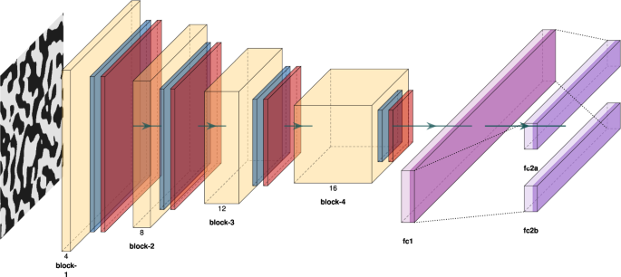

  

  Features are extracted from the microstructure x using a sequence of 4 blocks (each comprised of a sequence of convolutional layer, nonlinear activation function and pooling), where in each block the size of the feature map is reduced, while the depth of the feature map increases. Fully connected feedforward layers map the extracted convolutional features to the mean ${{{{\boldsymbol{m}}}}}_{{{{\boldsymbol{\theta }}}}}\left({{{\boldsymbol{x}}}}\right)$ and the covariance ${{{{\boldsymbol{S}}}}}_{{{{\boldsymbol{\theta }}}}}\left({{{\boldsymbol{x}}}}\right)$ of the predictive Gaussian distribution ${p}_{{{{\mathcal{M}}}}}\left({{{\boldsymbol{\kappa }}}}| {{{\boldsymbol{x}}}},{{{\boldsymbol{\theta }}}}\right)={{{\mathcal{N}}}}\left({{{\boldsymbol{\kappa }}}}| \,{{{{\boldsymbol{m}}}}}_{{{{\boldsymbol{\theta }}}}}\left({{{\boldsymbol{x}}}}\right),{{{{\boldsymbol{S}}}}}_{{{{\boldsymbol{\theta }}}}}\left({{{\boldsymbol{x}}}}\right)\right)$, where θ denotes the neural network parameters.

We note that the introduction of $p\left({{{\boldsymbol{\kappa }}}}| {{{\boldsymbol{x}}}}\right)$ and $p\left({{{\boldsymbol{x}}}}| \varphi \right)$ as a probabilistic representation of the PSP chain is a very general description which in principle can accommodate any epistemic or aleatoric source of uncertainty. With these definitions in hand, we proceed to define two closely related optimization problems (O1) and (O2) that we would like to address. For the first optimization problem (O1) we make use of a utility function u(${\boldsymbol{\kappa }}$) ≥ 0 (negative-valued utility functions can also be employed, as long as they are bounded from below). Due to the aforementioned uncertainties we consider the expected utility U₁(φ) which is defined as [Eq. 5]:

$${U}_{1}(\varphi )={{\mathbb{E}}}_{p\left({{{\boldsymbol{x}}}}| \varphi \right)}\left[\int u({{{\boldsymbol{\kappa }}}})\,p({{{\boldsymbol{\kappa }}}}| {{{\boldsymbol{x}}}})\,d{{{\boldsymbol{\kappa }}}}\right]$$

(5)

(where ${{\mathbb{E}}}_{p\left({{{\boldsymbol{x}}}}| \varphi \right)}[.]$ implies an expectation with respect to $p\left({{{\boldsymbol{x}}}}| \varphi \right)$) and seek the processing parameters φ that maximize it, i.e. [Eq. 6]:

$${{{\rm{(O1)}}}}:\qquad {\varphi }^{* }=\arg \mathop{\max }\limits_{\varphi }\,{U}_{1}\left(\varphi \right)$$

(6)

Consider for example the case that $u({{{\boldsymbol{\kappa }}}})={{\mathbb{I}}}_{{{{\mathcal{K}}}}}\left({{{\boldsymbol{\kappa }}}}\right)$, i.e., the indicator function of some target domain ${{{\mathcal{K}}}}$, defining the desired range of property values (Fig. 2a). In this case, solving (O1) above will lead to the value of φ that maximizes the probability that the resulting material will have properties in the target domain ${{{\mathcal{K}}}}$, i.e., ${U}_{1}\left(\varphi \right)=Pr\left({{{\boldsymbol{\kappa }}}}\in {{{\mathcal{K}}}}| \varphi \right)$. Similar probabilistic objectives have been proposed for several other materials’ classes and models (e.g.³⁵). Another possibility of potential practical interest involves introducing $u({{{\boldsymbol{\kappa }}}})={e}^{-\tau | | {{{\boldsymbol{\kappa }}}}-{{{{\boldsymbol{\kappa }}}}}_{target}| {| }^{2}}$, with τ a scaling parameter. In this case solving (O1) leads to the material with properties which, on average, are closest to the prescribed target ${\boldsymbol{\kappa }}_{target}$ (Fig. 2b).

The second problem we consider involves prescribing a target density p_target(${\boldsymbol{\kappa }}$) on the material properties and seeking the φ that leads to a marginal density of properties $p\left({{{\boldsymbol{\kappa }}}}| \varphi \right)={{\mathbb{E}}}_{p\left({{{\boldsymbol{x}}}}| \varphi \right)}\left[p\left({{{\boldsymbol{\kappa }}}}| {{{\boldsymbol{x}}}}\right)\right]$ that is as close as possible to this target (Fig. 2c). While there are several distance measures in the space of densities, we employ here the Kullback–Leibler divergence KL(p_target(${\boldsymbol{\kappa }}$)∣∣p(${\boldsymbol{\kappa }}$∣φ)), the minimization of which is equivalent to (see Supplementary Notes) [Eq. 7]:

$$\begin{array}{lll}{{{\rm{(O2)}}}}:\qquad {\varphi }^{* }&=&\arg \mathop{\max }\nolimits_{\varphi }{U}_{2}(\varphi )\\ {{{\rm{where}}}}\,{U}_{2}(\varphi )&=&\int {p}_{target}({{{\boldsymbol{\kappa }}}})\log p({{{\boldsymbol{\kappa }}}}| \varphi )\,d{{{\boldsymbol{\kappa }}}}\end{array}$$

(7)

The aforementioned objective resembles the one employed in¹⁷, but rather than finding a density on the microstructure (or features thereof) that leads to a close match of p_target (${\boldsymbol{\kappa }}$), we identify the processing variables φ that do so (i.e., we are a-priori constrained to distributions realizable for specific processing conditions φ).

We note that both problems are considerably more challenging than deterministic counterparts, as in both cases the objectives involve expectations with respect to the high-dimensional vector(s) x (and potentially ${\boldsymbol{\kappa }}$), representing the microstructure (and their effective properties). Additionally, in the case of (O2), the analytically intractable density $p\left({{{\boldsymbol{\kappa }}}}| \varphi \right)$ appears explicitly in the objective. While one might argue that a brute-force Monte Carlo approach with a sufficiently large number of samples would suffice to carry out the aforementioned integrations, we note that propagating the uncertainty from x to the properties ${\boldsymbol{\kappa }}$ would also require commensurate solutions of the expensive structure-property model which would need to be repeated for various φ-values. To overcome challenges associated with the structure-property link, we make use of a probabilistic surrogate model ${{{\mathcal{M}}}}$ trained on data ${{{\mathcal{D}}}}$ with a predictive density ${p}_{{{{\mathcal{M}}}}}({{{\boldsymbol{\kappa }}}}| {{{\boldsymbol{x}}}},{{{\mathcal{D}}}})$, which we use in place of the true $p\left({{{\boldsymbol{\kappa }}}}| \varphi \right)$ in the expressions above.

We note that an alternative strategy based on circumventing the high-dimensional x and trying to approximate directly $p\left({{{\boldsymbol{\kappa }}}}| \varphi \right)$³⁶, while tempting, will quickly become infeasible in terms of data requirements (i.e., triplets of (φ, x, ${\boldsymbol{\kappa }}$)) even for modest dimensions of φ. The reformulated objectives based on ${p}_{{{{\mathcal{M}}}}}\left({{{\boldsymbol{\kappa }}}}| {{{\boldsymbol{x}}}},{{{\mathcal{D}}}}\right)$ are denoted with ${U}_{1,{{{\mathcal{M}}}}}^{{{{\mathcal{D}}}}}$ and ${U}_{2,{{{\mathcal{M}}}}}^{{{{\mathcal{D}}}}}$. We discuss the solution strategy of the optimization problem as well as the specifics of the probabilistic surrogate in the next sections.

Expectation-maximization and stochastic variational inference

We present the proposed algorithm for the solution of (O1) and discuss the requisite changes for (O2) afterward. The goal to identify the optimal process parameters φ* remains challenging despite the introduction of an inexpensive, probabilistic surrogate, since the the objective functions as well as their derivatives remain intractable due to the averaging over the high-dimensional microstructures x, as well as the—in the general case—intractable integration over ${\boldsymbol{\kappa }}$ in Eq. (5). For this reason we propose to employ the Expectation-Maximization scheme³⁷, which is based on the so-called Evidence Lower BOund (ELBO) ${{{\mathcal{F}}}}$ [Eq. 8]:

$$\begin{array}{lll}\log {U}_{1,{{{\mathcal{M}}}}}^{{{{\mathcal{D}}}}}(\varphi )&=\log \int u({{{\boldsymbol{\kappa }}}})\,{p}_{{{{\mathcal{M}}}}}({{{\boldsymbol{\kappa }}}}| {{{\boldsymbol{x}}}},{{{\mathcal{D}}}})\,p({{{\boldsymbol{x}}}}| \varphi )\,d{{{\boldsymbol{\kappa }}}}\,d{{{\boldsymbol{x}}}}\\ &\ge {{\mathbb{E}}}_{q({{{\boldsymbol{x}}}},{{{\boldsymbol{\kappa }}}})}\left[\log \frac{u({{{\boldsymbol{\kappa }}}})\,{p}_{{{{\mathcal{M}}}}}({{{\boldsymbol{\kappa }}}}| {{{\boldsymbol{x}}}},{{{\mathcal{D}}}})\,p({{{\boldsymbol{x}}}}| \varphi )}{q({{{\boldsymbol{x}}}},{{{\boldsymbol{\kappa }}}})}\right]\\ &={{{\mathcal{F}}}}\left(q\left({{{\boldsymbol{\kappa }}}},{{{\boldsymbol{x}}}}\right),\varphi \right)\end{array}$$

(8)

where ${{\mathbb{E}}}_{q({{{\boldsymbol{x}}}},{{{\boldsymbol{\kappa }}}})}[.]$ denotes an expectation with respect to the auxiliary density q(x, ${\boldsymbol{\kappa }}$). The algorithm alternates between maximizing ${{{\mathcal{F}}}}$ with respect to the density q(x, ${\boldsymbol{\kappa }}$) while φ is fixed (E-step) and maximizing with respect to φ (M-step) while q(x, ${\boldsymbol{\kappa }}$) is fixed. We employ a Variational-Bayesian relaxation³⁸, in short VB-EM, according to which instead of the optimal q we consider a family ${{{{\mathcal{Q}}}}}_{{{{\boldsymbol{\xi }}}}}$ of densities parameterized by ξ and in the E-step maximize ${{{\mathcal{F}}}}$ with respect to ξ. This, as well as the the maximization with respect to φ in the M-step, are done by using stochastic gradient ascent where the associated derivatives are substituted by noisy Monte Carlo estimates (i.e., SVI¹⁶). The particulars of ξ as well as of the E- and M-steps are discussed in the Supplementary Notes. We illustrate the basic, numerical steps in the inner-loop of Algorithm (1) (the algorithm starts from an initial, typically random, guess of ξ and φ). Colloquially, the VB-EM iterations can be explained as follows: In the E-step and given the current estimate for φ, one averages over microstructures that are not only a priori more probable according to p(x∣φ) but also achieve a higher score according to $u({{{\boldsymbol{\kappa }}}})\,{p}_{{{{\mathcal{M}}}}}({{{\boldsymbol{\kappa }}}}| {{{\boldsymbol{x}}}},{{{\mathcal{D}}}})$. Subsequently, in the M-step step, we update the optimization variables φ on the basis of the average above (see Supplementary Notes for further details).

The second objective, ${U}_{2,{{{\mathcal{M}}}}}$ (Eq. (7)) can be dealt with in a similar fashion. The integration over ${\boldsymbol{\kappa }}$ with respect to the target density ${p}_{target}\left({{{\boldsymbol{\kappa }}}}\right)$ is first approximated using S Monte Carlo samples ${\{{{{{\boldsymbol{\kappa }}}}}^{(s)}\}}_{s = 1}^{S}$ from ${p}_{target}\left({{{\boldsymbol{\kappa }}}}\right)$, and subsequently each of the terms in the sum can be lower-bounded as follows [Eq. 9]:

$$\begin{array}{lll}{U}_{2,{{{\mathcal{M}}}}}^{{{{\mathcal{D}}}}}(\varphi )=\int {p}_{target}({{{\boldsymbol{\kappa }}}})\log {p}_{{{{\mathcal{M}}}}}({{{\boldsymbol{\kappa }}}}| \varphi ,{{{\mathcal{D}}}})\,d{{{\boldsymbol{\kappa }}}}\\\qquad\qquad \approx \frac{1}{S}\mathop{\sum }\nolimits_{s = 1}^{S}\log {p}_{{{{\mathcal{M}}}}}({{{{\boldsymbol{\kappa }}}}}^{(s)}| \varphi ,{{{\mathcal{D}}}})\\ \qquad\qquad=\frac{1}{S}\mathop{\sum }\nolimits_{s = 1}^{S}\log \int {p}_{{{{\mathcal{M}}}}}({{{{\boldsymbol{\kappa }}}}}^{(s)}| {{{\boldsymbol{x}}}},{{{\mathcal{D}}}})\,p({{{\boldsymbol{x}}}}| \varphi )\,d{{{\boldsymbol{x}}}}\\ \qquad\qquad \ge \frac{1}{S}\mathop{\sum }\nolimits_{s = 1}^{S}{{\mathbb{E}}}_{{q}^{(s)}({{{\boldsymbol{x}}}})}\left[\log \frac{{p}_{{{{\mathcal{M}}}}}({{{{\boldsymbol{\kappa }}}}}^{(s)}| {{{\boldsymbol{x}}}},{{{\mathcal{D}}}})\,p({{{\boldsymbol{x}}}}| \varphi )}{{q}^{(s)}({{{\boldsymbol{x}}}})}\right]\\ \qquad\qquad=\frac{1}{S}\mathop{\sum }\nolimits_{s = 1}^{S}{{{{\mathcal{F}}}}}_{s}\left({q}^{(s)}\left({{{\boldsymbol{x}}}}\right),\varphi \right)\end{array}$$

(9)

In this case, the aforementioned SVI tools will need to be applied for updating each ${q}^{(s)}\left({{{\boldsymbol{x}}}}\right),s=1,...\,,S$ in the E-step, but the overall algorithm remains conceptually identical. We note that incremental and partial versions of the EM-algorithm are possible, where e.g., one or more steps of stochastic gradient ascent are performed for a subset of the q^(s)39, leading to overall improved computational performance.

Probabilistic surrogate model

Despite the introduction of densities in the VB-EM algorithm which are tailored to the optimization problem and which enable accurate Monte Carlo estimates of the high-dimensional integrations involved, multiple evaluations of the S-P link are still required. To that end, the high-fidelity model (i.e., ${\boldsymbol{\kappa }}$(x) or $p\left({{{\boldsymbol{\kappa }}}}| \varphi \right)$), is substituted by a data-driven surrogate (i.e., ${p}_{{{{\mathcal{M}}}}}\left({{{\boldsymbol{\kappa }}}}| {{{\boldsymbol{x}}}},{{{\mathcal{D}}}}\right)$) which is trained on N pairs [Eq. 10]

$${{{\mathcal{D}}}}={\left\{{{{{\boldsymbol{x}}}}}^{(n)},{{{{\boldsymbol{\kappa }}}}}^{(n)} = {{{\boldsymbol{\kappa }}}}\left({{{{\boldsymbol{x}}}}}^{(n)}\right)\right\}}_{n = 1}^{N}$$

(10)

generated by the deterministic/stochastic high-fidelity model. While such supervised machine-learning problems have been studied extensively and a lot of the associated tools have found their way in materials applications⁴⁰, we note that their use in the context of the optimization problems presented requires significant adaptations.

In particular, and unlike canonical, data-centric applications relying on the abundance of data (Big Data), we operate under a smallest-possible-data regime. This is because in our setting training data arises from expensive simulations, the number of which we want to minimize. The shortage of information generally leads to predictive uncertainty (even for deterministic S-P links) which, rather than dismissing, we quantify by employing a probabilistic surrogate that yields a predictive density ${p}_{{{{\mathcal{M}}}}}({{{\boldsymbol{\kappa }}}}| {{{\boldsymbol{x}}}},{{{\mathcal{D}}}})$ instead of mere point estimates. More importantly though, we note that the distribution of the inputs in ${{{\mathcal{D}}}}$, i.e., the microstructures x, changes drastically with φ (Fig. 1). As we do not know a priori the optimal φ*, we cannot generate training data from $p\left({{{\boldsymbol{\kappa }}}}| \varphi^* \right)$. At the same time it is well known that data-driven surrogates produce poor extrapolative, out-of-distribution predictions⁴¹. It is clear therefore, that the selection of the training data, i.e., the microstructures-inputs x⁽ⁿ⁾ for which we pay the price of computing the output-property of interest ${\boldsymbol{\kappa }}^{(n)}$, should be informed by the optimization algorithm in order to produce a sufficiently accurate surrogate while keeping N as small as possible. We defer a detailed discussion of this aspect for the next section, and first present the particulars of the surrogate model employed.

The probabilistic surrogate ${{{\mathcal{M}}}}$ adopted has a Gaussian likelihood, i.e., ${p}_{{{{\mathcal{M}}}}}({{{\boldsymbol{\kappa }}}}| {{{\boldsymbol{x}}}})={{{\mathcal{N}}}}\left({{{\boldsymbol{\kappa }}}}| {{{{\boldsymbol{m}}}}}_{{{{\boldsymbol{\theta }}}}}({{{\boldsymbol{x}}}}),{{{{\boldsymbol{S}}}}}_{{{{\boldsymbol{\theta }}}}}({{{\boldsymbol{x}}}})\right)$, where the mean m_θ(x) and covariance S_θ(x) are modeled with a convolutional neural network (CNN) (see Fig. 9 and Supplementary Notes for more details), with θ denoting the associated neural network parameters. CNNs have been used previously for property prediction in binary media in e.g.,^42,43. Point estimates ${{{{\boldsymbol{\theta }}}}}_{{{{\mathcal{D}}}}}$ of the parameters are obtained with the help of training data ${{{\mathcal{D}}}}$ by maximizing the corresponding likelihood ${p}_{{{{\mathcal{M}}}}}\left({{{\mathcal{D}}}}| {{{\boldsymbol{\theta }}}}\right)=\mathop{\prod }\nolimits_{n = 1}^{N}{{{\mathcal{N}}}}\left({{{{\boldsymbol{\kappa }}}}}^{(n)}| {{{{\boldsymbol{m}}}}}_{{{{\boldsymbol{\theta }}}}}({{{{\boldsymbol{x}}}}}^{(n)}),{{{{\boldsymbol{S}}}}}_{{{{\boldsymbol{\theta }}}}}({{{{\boldsymbol{x}}}}}^{(n)})\right)$. On the basis of these estimates, the predictive density (i.e for a new input-microstructure x) of the surrogate follows as ${p}_{{{{\mathcal{M}}}}}({{{\boldsymbol{\kappa }}}}| {{{\boldsymbol{x}}}},{{{\mathcal{D}}}})={{{\mathcal{N}}}}\left({{{\boldsymbol{\kappa }}}}| {{{{\boldsymbol{m}}}}}_{{{{{\boldsymbol{\theta }}}}}_{{{{\mathcal{D}}}}}}({{{\boldsymbol{x}}}}),{{{{\boldsymbol{S}}}}}_{{{{{\boldsymbol{\theta }}}}}_{{{{\mathcal{D}}}}}}({{{\boldsymbol{x}}}})\right)$. We emphasize the dependence of the probabilistic surrogate on the dataset ${{{\mathcal{D}}}}$, for which we will discuss an adaptive acquisition strategy in the following section. While the results obtained are based on this particular architecture of the surrogate, the methodological framework proposed can accommodate any probabilistic surrogate and integrate its predictive uncertainty in the optimization procedure. Similarly, the same data-based approach could also be adopted for $p\left({{{\boldsymbol{x}}}}| \varphi \right)$.

Active learning

Active learning refers to a family of methods whose goal is to improve learning accuracy and efficiency by selecting particularly salient training data⁴⁴. This is especially relevant in our application, in which the acquisition of data is de facto the most computationally expensive component. The basis of all such methods is to progressively enrich the training dataset by scoring candidate inputs (i.e., microstructures x in our case) based on their expected informativeness⁴⁵. The latter can be quantified with a so-called acquisition function α(x), for which many different forms have been proposed (depending on the specific setting). We note though that in most cases in the literature, acquisition functions associated with the predictive accuracy of the supervised learning model have been employed, which in our formulation translates to the accuracy of our surrogate in predicting the properties ${\boldsymbol{\kappa }}$ for an input-microstructure. Alternate acquisition functions have been proposed in the context of Bayesian Optimization problems which as explained in the introduction exhibit significant differences with ours¹¹. While it is true that a perfect surrogate (i.e., if $p({{{\boldsymbol{\kappa }}}}| {{{\boldsymbol{x}}}})={p}_{{{{\mathcal{M}}}}}({{{\boldsymbol{\kappa }}}}| {{{\boldsymbol{x}}}},{{{\mathcal{D}}}})\,\forall {{{\boldsymbol{x}}}}$) would yield the exact optimum, this is not a necessary condition. An approximate surrogate is sufficient, as long as its aggregate predictions can correctly guide the search in the φ-space in order to discover the optimal value of φ for (O1) or (O2). This also implies that an accurate surrogate for φ − values (and corresponding microstructures x) far away from the optimum is not necessary. The difficulty of course is that we do not know a priori what is the optimum φ* and a surrogate trained on microstructures drawn from p(x∣φ⁽⁰⁾) (with φ⁽⁰⁾ being the initial guess in the optimization—see Algorithm (1)) will generally perform poorly at other φ’s.

The acquisition function that we propose incorporates the optimization objectives. In particular, for the (O1) problem (Eq. (5)) it is given by:

$$\alpha ({{{\boldsymbol{x}}}})={{{\mbox{Var}}}}_{{p}_{{{{\mathcal{M}}}}}({{{\boldsymbol{\kappa }}}}| {{{\boldsymbol{x}}}},{{{\mathcal{D}}}})}\left[u({{{\boldsymbol{\kappa }}}})\right]$$

(11)

We note that α scores each microstructure x in terms of the predictive uncertainty in the utility u (the expected value of which we seek to maximize) due to the predictive density of the surrogate. In the case discussed earlier where $u({{{\boldsymbol{\kappa }}}})={{\mathbb{I}}}_{{{{\mathcal{K}}}}}\left({{{\boldsymbol{\kappa }}}}\right)$ (and ${U}_{1}(\varphi )=Pr\left({{{\boldsymbol{\kappa }}}}\in {{{\mathcal{K}}}}| \varphi \right)$), the acquisition function reduces to the variance of the event ${{{\boldsymbol{\kappa }}}}\in {{{\mathcal{K}}}}$. This suggests that the acquisition function yields the largest scores for microstructures for which the surrogate is most uncertain whether their corresponding properties fall within the target domain ${{{\mathcal{K}}}}$.

We propose a general procedure according to which the VB-EM-based optimization is embedded in an outer loop indexed by the data augmentation steps l = 1, . . . L. Hence ${{{{\mathcal{D}}}}}^{(l)}$ denotes the training dataset at step l, ${p}_{{{{\mathcal{M}}}}}({{{\boldsymbol{\kappa }}}}| {{{\boldsymbol{x}}}},{{{{\mathcal{D}}}}}^{(l)})$ the corresponding predictive density of the surrogate, q^(l)(x) the marginal variational density found in the last E-step and φ^(l) the optimum found in the last M-step. With this notation in hand we can then summarize the adaptive data augmentation as follows (see also Algorithm (1) in Fig. 10):

• in each outer loop iteration l we randomly generate a pool of candidate microstructures ${\{{{{{\boldsymbol{x}}}}}^{(l,n)}\}}_{n = 1}^{{N}_{pool}}$ from q^(l)(x) and select a subset of N_add < N_pool microstructures which yield the highest values of the acquisition function α(x^(l, n)).

• We solve the high-fidelity model for the aforementioned N_add microstructures and construct a new training dataset ${D}_{add}^{(l)}$ which we add to ${{{{\mathcal{D}}}}}^{(l)}$ in order to form ${{{{\mathcal{D}}}}}^{(l+1)}={{{{\mathcal{D}}}}}^{(l)}\cup {D}_{add}^{(l)}$. We retrain the surrogate based on ${{{{\mathcal{D}}}}}^{(l+1)}$, i.e., we compute ${p}_{{{{\mathcal{M}}}}}({{{\boldsymbol{\kappa }}}}| {{{\boldsymbol{x}}}},{{{{\mathcal{D}}}}}^{(l+1)})$, and restart the VB-EM-based optimization algorithm with the updated surrogate (we note that retraining could be avoided by making use of online learning⁴⁶, which can accomodate incremental adaptions of the dataset).

Fig. 10: Pseudo-code for proposed algorithm.

The inner VB-EM iterations are wrapped within the adaptive data acquisition as an outer loop.

For the (O2) problem we propose to select microstructures that yield the highest predictive log-score on the sample representation ${\{{{{{\boldsymbol{\kappa }}}}}^{(s)}\}}_{s = 1}^{S}$ of the target distribution, i.e. [Eq. 12],

$$\begin{array}{r}\alpha\, \left({{{\boldsymbol{x}}}}\right)=\frac{1}{S}\mathop{\sum }\limits_{s=1}^{S}\log {p}_{{{{\mathcal{M}}}}}\left({{{{\boldsymbol{\kappa }}}}}^{(s)}| {{{\boldsymbol{x}}}}\right)\qquad {{{{\boldsymbol{\kappa }}}}}^{(s)} \sim {p}_{target}\left({{{\boldsymbol{\kappa }}}}\right)\end{array}$$

(12)

References

National Science and Technology Council. Materials Genome Initiative for Global Competitiveness (Executive Office of the President, National Science and Technology Council, 2011).
McDowell, D. L. et al. Integrated design of multiscale, multifunctional materials and products (Butterworth-Heinemann, 2009).
Arróyave, R. & McDowell, D. L. Systems approaches to materials design: Past, present, and future. Annu. Rev. Mater. Res. 49, 103–126 (2019).
Chernatynskiy, A., Phillpot, S. R. & LeSar, R. Uncertainty quantification in multiscale simulation of materials: a prospective. Annu. Rev. Mater. Res. 43, 157–182 (2013).
Honarmandi, P. & Arróyave, R. Uncertainty quantification and propagation in computational materials science and simulation-assisted materials design. Integr. Mater. Manuf. Innov. 9, 103–143 (2020).
Liu, X., Furrer, D., Kosters, J. & Holmes, J. NASA Vision 2040: A Roadmap for Integrated, Multiscale Modeling and Simulation of Materials and Systems. Tech. Rep. https://ntrs.nasa.gov/citations/20180002010 (2018).
Bock, F. E. et al. A review of the application of machine learning and data mining approaches in continuum materials mechanics. Front. Mater. 6, https://www.frontiersin.org/article/10.3389/fmats.2019.00110 (2019).
Panchal, J. H., Kalidindi, S. R. & McDowell, D. L. Key computational modeling issues in integrated computational materials engineering. Comput. -Aided Des. 45, 4–25 (2013).
Grigo, C. & Koutsourelakis, P.-S. Bayesian model and dimension reduction for uncertainty propagation: applications in random media. SIAM/ASA J. Uncertain. Quantif. 7, 292–323 (2019).
Zabaras, N. & Ganapathysubramanian, B. A scalable framework for the solution of stochastic inverse problems using a sparse grid collocation approach. J. Comput. Phys. 227, 4697–4735 (2008).
Frazier, P. I. & Wang, J. Bayesian optimization for materials design. In Information Science for Materials Discovery and Design, 45–75 (Springer, 2015).
Zhang, Y., Apley, D. W. & Chen, W. Bayesian optimization for materials design with mixed quantitative and qualitative variables. Sci. Rep. 10, 4924 (2020).
Jung, J., Yoon, J. I., Park, H. K., Jo, H. & Kim, H. S. Microstructure design using machine learning generated low dimensional and continuous design space. Materialia 11, 100690 (2020).
Chen, C.-T. & Gu, G. X. Machine learning for composite materials. MRS Commun. 9, 556–566 (2019).
Torquato, S. Optimal design of heterogeneous materials. Annu. Rev. Mater. Res. 40, 101–129 (2010).
Hoffman, M. D., Blei, D. M., Wang, C. & Paisley, J. Stochastic Variational Inference. J. Mach. Learn. Res. 14, 1303–1347 (2013).
Tran, A. & Wildey, T. Solving stochastic inverse problems for Property–Structure linkages using data-consistent inversion and machine learning. Jom-us. 73, 72–89 (2020).
Nosouhi Dehnavi, F., Safdari, M., Abrinia, K., Hasanabadi, A. & Baniassadi, M. A framework for optimal microstructural design of random heterogeneous materials. Comput. Mech. 66, 123–139 (2020).
Acar, P., Srivastava, S. & Sundararaghavan, V. Stochastic design optimization of microstructures with utilization of a linear solver. AIAA J. 55, 3161–3168 (2017).
Acar, P. & Sundararaghavan, V. Stochastic design optimization of microstructural features using linear programming for robust design. AIAA J. 57, 448–455 (2019).
Liu, R. et al. A predictive machine learning approach for microstructure optimization and materials design. Sci. Rep. 5, 1–12 (2015).
Paul, A. et al. Microstructure optimization with constrained design objectives using machine learning-based feedback-aware data-generation. Nato. Sc. S. Ss. Iii. C. S. 160, 334–351 (2019).
Teubner, M. Level surfaces of Gaussian random fields and microemulsions. Europhys. Lett. 14, 403–408 (1991).
Roberts, A. P. & Teubner, M. Transport properties of heterogeneous materials derived from Gaussian random fields: Bounds and simulation. Phys. Rev. E 51, 4141–4154 (1995).
Koutsourelakis, P. Probabilistic characterization and simulation of multi-phase random media. Probabilist. Eng. Mech. 21, 227–234 (2006).
Bostanabad, R., Bui, A. T., Xie, W., Apley, D. W. & Chen, W. Stochastic microstructure characterization and reconstruction via supervised learning. Acta Mater. 103, 89–102 (2016).
Cang, R. et al. Microstructure representation and reconstruction of heterogeneous materials via deep belief network for computational material design. J. Mech. Design 139, https://asmedigitalcollection.asme.org/mechanicaldesign/articleabstract/139/7/071404/383783/Microstructure-Representation-and-Reconstruction (2017).
Miehe, C. & Koch, A. Computational micro-to-macro transitions of discretized microstructures undergoing small strains. Arch. Appl. Mech. 72, 300–317 (2002).
Hill, R. On constitutive macro-variables for heterogeneous solids at finite strain. Proc. R. Soc. A: Math. Phys. Eng. Sci. 326, 131–147 (1972).
Saheli, G., Garmestani, H. & Adams, B. L. Microstructure design of a two phase composite using two-point correlation functions. J. Comput. -Aided Mater. Des. 11, 103–115 (2004).
Fullwood, D. T., Niezgoda, S. R., Adams, B. L. & Kalidindi, S. R. Microstructure sensitive design for performance optimization. Prog. Mater. Sci. 55, 477–562 (2010).
Sternfels, R. & Koutsourelakis, P.-S. Stochastic design and control in random heterogeneous materials. Int. J. Multiscale Com. 9, 425–443 (2011).
Popova, E. et al. Process-structure linkages using a data science approach: application to simulated additive manufacturing data. Integr. Mater. Manuf. Innov. 6, 54–68 (2017).
Lee, X. Y. et al. Fast inverse design of microstructures via generative invariance networks. Nat. Comput. Sci. 1, 229–238 (2021).
Ikebata, H., Hongo, K., Isomura, T., Maezono, R. & Yoshida, R. Bayesian molecular design with a chemical language model. J. Comput. Aided Mol. Des. 31, 379–391 (2017).
Dempster, A. P., Laird, N. M. & Rubin, D. B. Maximum likelihood from incomplete data via the EM algorithm (with discussion). J. R. Stat. Soc. Ser. B 39, 1–38 (1977).
Beal, M. J. & Ghahramani, Z. Variational Bayesian learning of directed graphical models with hidden variables. Bayesian Anal. 1, 793–832 (2006).
Neal, R. M. & Hinton, G. E. A view of the em algorithm that justifies incremental, sparse, and other variants. In: Learning in Graphical Models, MIT Press, 355–368 (1998).
Kalidindi, S. R. A Bayesian framework for materials knowledge systems. MRS Commun. 9, 518–531 (2019).
Marcus, G. & Davis, E. Rebooting AI: Building Artificial Intelligence We Can Trust (Vintage, 2019).
Yang, Z. et al. Deep learning approaches for mining structure-property linkages in high contrast composites from simulation datasets. Nato. Sc. S. Ss. Iii. C. S. 151, 278–287 (2018).
Cecen, A., Dai, H., Yabansu, Y. C., Kalidindi, S. R. & Song, L. Material structure-property linkages using three-dimensional convolutional neural networks. Acta Mater. 146, 76–84 (2018).
Tong, S. Active Learning: Theory and Applications. Dissertation, Stanford University. https://scholar.google.de/scholar?hl=de&as_sdt=0%2C5&q=Active+learning%3A+Theory+and+applications&btnG (2001).
MacKay, D. J. C. Information-based objective functions for active data selection. Neural Comput. 4, 590–604 (1992).
Sahoo, D., Pham, Q., Lu, J. & Hoi, S. C. H. Online deep learning: learning deep neural networks on the fly. In: Proceedings of the Twenty-Seventh International Joint Conference on Artificial Intelligence Organization, 2660–2666. https://www.ijcai.org/proceedings/2018/369 (2018).
Acknowledgements
Funded under the Excellence Strategy of the Federal Government and the Länder in the context of the ARTEMIS Innovation Network.
Funding
Open Access funding enabled and organized by Projekt DEAL.
Author information
Authors and Affiliations
Contributions
M.R.: conceptualization, physics and machine-learning modeling and computations, algorithmic and code development, writing of the paper. P-S.K: conceptualization, writing of the paper.
Corresponding author
Ethics declarations
Competing interests
The authors declare no competing interests.
Additional information
Publisher’s note Springer Nature remains neutral with regard to jurisdictional claims in published maps and institutional affiliations.
Rights and permissions
Open Access This article is licensed under a Creative Commons Attribution 4.0 International License, which permits use, sharing, adaptation, distribution and reproduction in any medium or format, as long as you give appropriate credit to the original author(s) and the source, provide a link to the Creative Commons license, and indicate if changes were made. The images or other third party material in this article are included in the article’s Creative Commons license, unless indicated otherwise in a credit line to the material. If material is not included in the article’s Creative Commons license and your intended use is not permitted by statutory regulation or exceeds the permitted use, you will need to obtain permission directly from the copyright holder. To view a copy of this license, visit http://creativecommons.org/licenses/by/4.0/.
About this article
Cite this article
Rixner, M., Koutsourelakis, PS. Self-supervised optimization of random material microstructures in the small-data regime. npj Comput Mater 8, 46 (2022). https://doi.org/10.1038/s41524-022-00718-6
Received:
Accepted:
Published:
DOI: https://doi.org/10.1038/s41524-022-00718-6