Measuring distances in proteins by saturation-recovery EPR

Abstract

We describe a protocol for detecting electron spin–spin interactions between a radical and a metal ion in a protein or protein complex by saturation-recovery electron paramagnetic resonance (EPR). This protocol can be used with a protein containing an endogenous metal center and either an endogenous or synthetic radical species. We suggest a two-step approach whereby dipole–dipole or exchange interactions are first detected by continuous-wave EPR experiments and then quantified by saturation-recovery EPR. The latter measurements make it possible to measure long distances to within a few Ångstroms. The protocol for making distance measurements by saturation-recovery EPR will take approximately 6 days to complete.

Introduction

The techniques that first come to mind when thinking about protein structure determination are usually solution-state NMR or X-ray crystallography. However, a complete protein structure is not always available or necessary to answer some of the most interesting biophysical questions. Sometimes, the measurement of one distance (or a few) is sufficient to establish the plausibility of a mechanism or corroborate a proposed structure. If a protein or protein complex contains a metal-binding site and a radical species, the magnetic interaction between the unpaired electrons at these two sites can be detected and quantified by saturation-recovery EPR and the resulting data used to measure distances of ∼10–40 Å (refs. 1,2). Enzymes with multiple redox-active cofactors such as photosystem II (PSII) and ribonucleotide reductase (RNR) are obvious targets for this methodology^3,4. Indeed, in these systems, saturation-recovery EPR may also be used to measure exchange couplings between redox partners⁴. However, saturation-recovery EPR can also be used to measure distances between an endogenous metal-binding site and a strategically placed spin label to yield structural information⁵.

Long distances in macromolecules have been successfully measured using fluorescence resonance energy transfer^6,7,8 and by pulsed EPR methods such as double quantum coherence, “2 + 1,” and DEER sequences that use a pair of spin labels (radicals)^9,10,11. Distance measurement by saturation recovery has an advantage over these other methods when the protein contains an endogenous paramagnetic metal center in that the protein has a built-in “label.” The other label, that is, the radical, may be either endogenous or introduced through spin-labeling methods^12,13,14. Additionally, in the case where the paramagnetic metal center is itself of interest, the radical can serve as a reporter of its magnetic properties. For example, in our experiments with the B2 subunit of RNR, the stable tyrosine radical was used to determine the exchange coupling within the dinuclear iron center⁴.

As pulsed EPR instruments are not yet as common as pulsed (Fourier-transform) NMR instruments, we recommend that the investigator first attempts to detect the presence of electron spin–spin interactions using the more common continuous-wave (CW) EPR spectrometer. This is done via the microwave progressive power saturation experiment. Although a protocol for this experiment is not provided here, we describe the experimental method in sufficient detail that the investigator with some CW EPR experience should be able to execute the experiment. Once the investigator has detected a spin–spin interaction between the radical and the metal center, he or she may want to enlist the assistance of an experienced EPR spectroscopist before performing the saturation-recovery experiment. Although this experiment is not particularly difficult to set up, pulsed EPR spectrometers lack some of the safeguards found on modern NMR spectrometers that prevent damage to the instrument.

The sample preparation steps described in this protocol are appropriate for both the microwave progressive power saturation experiment (CW EPR) and the saturation-recovery EPR experiment. Note that some method for cooling the sample to cryogenic temperatures is required for both the CW and saturation-recovery EPR experiments. A variable-temperature helium cryostat is recommended for the CW EPR experiments and required for the saturation-recovery EPR experiments. Although a liquid nitrogen finger Dewar can provide only a single cryogenic temperature (77 K), this may be sufficient to establish the presence of electron spin–spin interactions in the CW EPR experiment.

Spin–lattice relaxation

Imposing a static magnetic field on a sample containing unpaired electron spins causes the spins to orient either with or against the magnetic field. For electrons, orientation of the electron spins antiparallel to the imposed field is energetically more favorable, although the energy difference between parallel and antiparallel orientations, ΔE = hν, is small compared to the thermal energy of the system, k_BT (Fig. 1).

Figure 1: Energy diagram for radicals with a single unpaired electron (S = 1/2).

The equilibrium populations of the two spin states, +1/2 and −1/2, depend on the energy difference between them and the temperature. At any moment in time, some radicals will have their electron spins oriented parallel to the magnetic field (top) whereas others will have their electron spins oriented antiparallel to the magnetic field (bottom). At equilibrium, the antiparallel population is slightly greater since this orientation is lower in energy.

Here h is the Planck's constant, ν is the resonant frequency at the applied magnetic field, k_B is the Boltzmann constant and T the temperature in Kelvin. For radicals with a single unpaired electron, the relative populations in the two spin states at equilibrium is described by

where N_+1/2 and N_−1/2 are the populations of the parallel and antiparallel spin states, respectively. The magnitude of the signal observed in a magnetic resonance experiment is proportional to that of the magnetization along the z axis, M_z, where

Non-equilibrium spin populations can be produced by continuous irradiation of the spins at their resonant frequency or by a microwave pulse. Spin–lattice relaxation is the process by which the equilibrium populations of the spin states are restored. In a dilute solution, where the radicals are widely dispersed and unaffected by metal centers or other paramagnetic molecules, this process is characterized by a single rate constant, k₁, typically written as 1/T₁.

Dipole–dipole- and exchange-induced relaxation enhancement

In the methods discussed here, one detects the interaction of the radical with the metal center via the enhancement of the spin–lattice relaxation rate of the radical. There are two mechanisms by which the metal center can enhance the radical's spin–lattice relaxation rate^{15,16,17,18,19,20}. One mechanism is the dipole–dipole interaction, a through-space mechanism that only requires proximity between the radical and the metal center. It is by this mechanism that distances are measured. The other is the exchange interaction, a through-bond mechanism that requires either direct or indirect orbital overlap between the radical and the metal center. The exchange interaction is most likely to be a significant source of relaxation enhancement between redox partners at distances of ≤10 Å.

For spin–spin interactions over distances greater than 10 Å, where the absence of an exchange interaction can be assumed, the overall spin–lattice relaxation rate, k₁, of a radical in proximity to a paramagnetic metal center can be considered to be the sum of two rate constants:

The rate constant k_1i is the intrinsic spin–lattice relaxation rate, that is, the relaxation rate of the radical when not in proximity to other paramagnetic species. The intrinsic rate constant, k_1i, is taken to be independent of the protein's (radical's) orientation in the magnetic field. (Strictly speaking, there may be some orientation dependence to k_1i, but it is generally weak enough to be ignored.) The rate constant k_1θ represents the dipole–dipole-induced relaxation rate and is orientation dependent, that is, it depends on the angle θ formed by two vectors, the interspin vector that connects the radical to the metal center and the magnetic field vector (Fig. 2). As described below, the orientation dependence of this rate constant makes it possible to separate its contribution to k₁ from that of k_1i. If there is an exchange coupling between the two sites, it can contribute both an orientation-independent k_1ex and an orientation-dependent k_1ex(θ) term to equation (2). We will discuss, in qualitative terms, the effect that this can have in both the CW and saturation-recovery EPR data. However, we refer the reader to the appropriate equations in Rakowsky et al.²¹ should the exchange interaction make a measurable contribution to the spin–lattice relaxation.

Figure 2: The interspin vector r forms an angle θ with the static magnetic field H₀.

In the diagram, s represents the radical as it is the “slowly” relaxing spin and f represents the metal center as it is a “fast” relaxer. The relaxation enhancement provided by a dipole–dipole interaction depends on the angle θ.

The rate constants are a function of temperature. If a significant exchange interaction is present, then the rate constants arising from the exchange and the dipole–dipole interactions may have the same temperature dependence because they depend on the paramagnetic relaxation properties of the metal center. However, the intrinsic relaxation rate constant, k_1i, will typically have a different temperature dependence than the other rate constants because it arises from the spin–lattice relaxation of the radical itself²². This difference in temperature dependence means that the relative contribution of k_1i, k_1θ, k_1ex or k_1ex(θ) to the overall relaxation rate, k₁, can vary greatly with temperature.

Samples for the measurement of k_1i

The intrinsic relaxation rate constant for a particular radical species at a given temperature depends on the matrix surrounding the radical. (The surrounding matrix determines how well the electron spin transitions are coupled to the surrounding low-frequency vibrations of the sample.) Therefore, for an endogenous radical species, it is best to measure k_1i in the protein of interest. This requires that the metal center be rendered diamagnetic so that neither exchange nor dipole–dipole interactions enhance the spin–lattice relaxation rate. The metal center can be rendered diamagnetic by removing the paramagnetic metal ion or replacing it with a diamagnetic ion^23,24 or, in some instances, changing the metal ion's oxidation state or its ligands²⁵. However, if none of these options is workable, it may be possible to use the spin–lattice relaxation rates of the same radical species in (frozen) solution as k_1i (ref. 3). (See Fig. 3, for example, panel a, showing the saturation-recovery transient of L-tyrosine radical generated by UV irradiation of a frozen solution.) Note that even if a suitable system for measuring k_1i cannot be produced, it is still possible to detect the presence of a dipole–dipole interaction (see below)²⁶.

Figure 3: In the absence of electron spin–spin interactions, the saturation-recovery transients of tyrosine-based radicals are single-exponential.

Saturation-recovery transients of (a) the UV-generated tyrosine radical at 22 K and (b) the tyrosyl radical of the B2 subunit of RNR at 10 K with single-exponential fits superimposed. Note the different timescales. For the UV-generated tyrosine radical, the observing microwave power level was 2.0 μW and the saturating microwave pulse (63 mW) was of 8-ms duration. For the tyrosyl radical of the B2 subunit, the observing microwave power level was 0.23 μW and the saturating microwave pulse (160 mW) was of 100-ms duration⁴⁶.

CW EPR

Microwave progressive power saturation.

In the microwave progressive power saturation experiment, the peak-to-peak height of the first derivative CW EPR signal is measured as the microwave power (observe power) is increased. At low powers, when the equilibrium population of spin states remains unperturbed, the height of the signal increases in proportion to the square root of the power. As the observe power increases further, the signal becomes “saturated,” that is, N_+1/2/N_−1/2 approaches 1 because spin–lattice relaxation can no longer maintain the equilibrium population difference of the two spin states. Under these conditions, the signal height may continue to increase with increasing power, but a fourfold increase in power will yield less than a twofold increase in signal height. At very high powers, the signal intensity may actually decrease with increasing observe power. The following equation derived from the work of Portis²⁷ and Castner²⁸ describes the expected behavior:

where S′ is the first-derivative peak-to-peak height of the radical signal, K is a constant, P is the microwave power, P_1/2 is the power at half saturation and b is an adjustable parameter having a value between 3, for a purely homogeneously broadened line, and 1, for an inhomogeneously broadened line. Many radicals in frozen solution will be inhomogeneously broadened such that b≈1. In the absence of paramagnetic interactions between radicals or between radicals and metal ions, Figure 3, P_1/2 has a single value that can be determined by plotting the data as log(S′/√P) versus log(P). This yields two linear regions that intersect at P = P_1/2. Figure 4 shows an example of this plot. The limit P ≪ P_1/2 yields a horizontal line since S′/√P (and log(S′/√P)) is constant. The limit P ≫ P_1/2 yields a straight line with slope −b/2. The quantity P_1/2 is directly proportional to the product of k₁ and k₂, that is,

where k₁ is the spin–lattice relaxation rate and k₂ (1/T₂) is the spin–spin relaxation rate of the radical species.

Figure 4: Log–log plot showing microwave progressive power saturation data for EPR signals from (▪) the tyrosine radical Y_D^• in PSII depleted of manganese, (□) the UV-generated L-tyrosine radical and (•) the tyrosine radical in RNR from Escherichia coli at 7.0 K.

Y_D^• (▪) is a neutral tyrosine radical produced by illumination of PSII at low temperature. It experiences a dipole–dipole interaction with the non-heme Fe(II) that can be observed when paramagnetic manganese ions are removed from the oxygen-evolving complex. At this temperature, the dinuclear iron center of RNR is diamagnetic (S = 0). There are no paramagnetic metal ions present in the UV-generated L-tyrosine radical sample. When equation (4) was used to fit the data for the three radical species with b and P_1/2 as adjustable parameters, the values of b were 0.73, 1.03 and 0.95 for Y_D^• in PSII, the L-tyrosine radical and tyrosine radical from E. coli RNR, respectively. The lines are the best fits to the data with b = 1, the value of b at the limit of nonhomogeneous broadening. The vertical positions of the curves are offset arbitrarily. Conditions: field modulation width, 2.0 G; field modulation frequency, 100 kHz; microwave frequency, 9.05 GHz. Inset: CW first-derivative EPR spectrum of the stable tyrosine radical Y_D^• in PSII. The horizontal arrows mark the positions used to measure the peak-to-peak height S′. The vertical arrow marks the magnetic field position at which saturation-recovery transients were recorded³.

Detecting dipole–dipole and exchange couplings.

The microwave progressive power saturation curve can provide evidence for a dipole–dipole interaction if k_1θ is large compared to k_1i. Because the dipole–dipole interaction is orientation dependent, radicals with different orientations of the interspin vector in the magnetic field will have different values of k_1θ and, therefore, different values of k₁ (equation (3)). The result is that there is no single value of P_1/2 that can characterize the power at half saturation (equation (5)) but rather a range of values whose extent depends on the strength of the dipole–dipole interaction²⁹. The effect is to “stretch” the P_1/2 curve along the x axis (microwave power). The presence of this stretching can be confirmed by fitting the saturation curve (equation (4)) with “b” as an adjustable parameter. If the saturation curves of two samples of the same radical species are compared, one sample with a diamagnetic metal center (or no metal center) and one with a paramagnetic metal center, the fitted value of “b” will be smaller for the sample with the paramagnetic center (Fig. 4). If the only sample available is one with a paramagnetic metal center, the presence of a dipole–dipole interaction can still be inferred if the fitted value of b is less than 1, as this is below the limit for an inhomogeneously broadened line.

With a variable-temperature helium flow cryostat, a series of microwave progressive power saturation curves can be acquired, each at a different temperature. This allows the investigator to search for a temperature regime where k_1θ is large relative to k_1i. If a variable-temperature cryostat is not available, it may be possible to observe this effect at 77 K using a relatively inexpensive liquid nitrogen finger Dewar.

If k_1ex is larger than k_1θ, then the microwave progressive power saturation curves may not be detectably “stretched.” However, the magnitude of P_1/2 will be higher in the protein sample with a paramagnetic metal center than it will be in one with a diamagnetic metal center. Therefore, the magnitude of P_1/2 in the two samples can be used to detect an electron spin–spin interaction between the two sites. With two samples and a variable-temperature helium cryostat, the investigator can plot the calculated P_1/2 values versus temperature to determine the temperature point or region where maximal relaxation enhancement occurs.

Although relatively easy to perform, the microwave progressive power saturation experiment is not always easy to interpret. Because P_1/2 depends on the spin–spin relaxation rate constant, k₂, as well as on the spin–lattice relaxation constant, k₁, it may not be possible to determine which is responsible for increasing the magnitude of P_1/2. Indeed, although beyond the scope of our discussion here, k₂ can also be enhanced by exchange or dipole–dipole interactions^25,30. However, microwave progressive power saturation allows the detection of exchange- or dipole–dipole-induced enhancement of k₁ or k₂ and the temperature regions that produce the maximal effects. The investigator will then be well positioned to determine the source of relaxation enhancement in the saturation-recovery experiment.

The saturation-recovery experiment

We describe here methods for extracting a rate constant proportional to the distance between the radical and the metal center and then calculating the distance itself. For the investigator already acquainted with the fundamental theories describing NMR, the terms and concepts will be familiar. It is hoped that those unfamiliar with magnetic resonance will still be able to follow the basic outline of the experiment. We recommend the introductory NMR texts of Roberts³¹ and Harris³² and the EPR texts of Weil et al.³³ and Symons³⁴ to those interested in gaining some background in magnetic resonance.

The basic principle behind measuring distances by saturation-recovery EPR is straightforward. Using a pulsed EPR spectrometer, one first “saturates” the spins on resonance, that is, one equalizes the two populations N_+1/2 and N_−1/2 rendering the magnetic resonance signal equal to zero (equation (2)). The recovery of the equilibrium spin populations is then recorded via the return of the magnetic resonance signal to its full magnitude (Fig. 5). If done properly (see Supplementary Fig. 1 online), the observed rate of recovery is the spin–lattice relaxation rate, k₁.

Figure 5: The anatomy of a CW saturation-recovery experiment.

The defense pulse switches on before the high-power saturating pulse and stays on until a short time afterward (typically 1–5 ms) to protect the receiver electronics from microwave power reflected by the resonator. The saturating pulse stays on for a time equal to 1/k₁ (T₁) for the observed radical to minimize the effects of spectral diffusion (see Supplementary Fig. 1 online). The saturating pulse equalizes the populations in the two spin states, driving the observable magnetization to zero (top). The recovery of the equilibrium spin populations is recorded at low microwave observe power for a time equal to ∼5/k₁ (5T₁), producing a saturation-recovery transient. Note that the total time required for one complete pulse sequence (the shot recovery time) is 6/k₁ (6T₁) in both the CW saturation-recovery and the spin-echo saturation-recovery experiments to allow for the complete saturation of the radicals and suppression of spectral diffusion, 1/k₁, and their complete recovery to equilibrium, 5/k₁. The horizontal broken lines indicate the zero level or “off” state for each component of the pulse sequence. The vertical broken line indicates the start of data acquisition.

Consider the case of a radical in a protein, experiencing only a dipole–dipole interaction with a metal center in the same protein. For any one orientation of the interspin vector, the recovery of the equilibrium population distribution and the magnetic resonance signal, I, is described by the following equation:

For a single value of θ, there is a single value of k₁, and the recovery will be single exponential. However, in a frozen solution of protein, the angle θ can take on all values between 0 and π, and the observed recovery of the magnetic resonance signal will be the sum of these single-exponential recoveries, that is,

where sin θ gives the appropriate weighting to each angle θ and N is a normalization constant^3,35. To evaluate equation (7) and model the actual recovery, we must have an explicit equation for k_1θ. For the situation most likely to be encountered by the investigator, that is, a spectrometer operating at X-band (9 GHz) or higher, a metal center containing first row transition metals, and temperatures near or below that of liquid nitrogen, k_1θ can be expressed as^3,19,20

where the dipolar rate constant, k_1d, is defined by

where γ_s is the magnetogyric ratio of the radical (the slowly relaxing spin), μ_f is the magnetic dipole moment of the metal center (the fast relaxing spin), r is the distance between the radical and the metal center, ω_s equals 2πν, where ν is the resonant frequency of the radical, T_1f and T_2f are the spin–lattice and spin–spin relaxation times of the metal center, respectively, and g_s and g_f are the g values of the radical and metal center, respectively. For simplicity, we assume here that g_f is a single isotropic value. Others have taken the orientation dependence of g_f into account explicitly²¹.

There appear to be a great many terms in equations (8) and (9). However, γ_s, μ_f, ω_s, g_s and g_f can be determined from the CW EPR spectra of the radical and metal center. Furthermore, at temperatures between liquid helium and liquid nitrogen, it is likely that either the first or the second orientation-dependent term within brackets in equation (8) will dominate the relaxation, allowing the equation to be simplified. The first term in brackets will dominate the dipole–dipole relaxation enhancement if |(1 − gf/gs)| is significantly less than one and/or if T_1f /T_2f is significantly greater than one.

Equation (7) tells us that the recovery of the magnetization of the radicals will NOT be single exponential if the dipole–dipole-induced relaxation rate is comparable to or larger than the intrinsic relaxation rate. By substituting equation (8) into equation (7) and using equation (7) to fit the observed recovery of the magnetization, one can extract k_1d, the dipolar rate constant. Note that the integral in equation (7) cannot be solved analytically but can be evaluated numerically. This can be done most efficiently by writing the integral as a sum and then summing over equal increments of cos θ (ref. 26).

Once k_1d has been determined, there are two approaches to calculate r, the distance between the radical and metal center, using equation (9). One approach is to measure T_1f and T_2f directly or indirectly²¹. Near liquid helium temperatures, it may be possible to measure T_1f and T_2f of the metal center using the saturation-recovery experiment and spin-echo experiments, respectively. However, instrumental limitations make it difficult to measure relaxation times below ∼1 μs, and at these “long” values of T_1f and T_2f, the relaxation enhancement induced by the dipole–dipole interaction may be detectable for only “shorter” distances near 10 Å. At higher temperatures and shorter relaxation times, it may be possible to estimate T_1f by analyzing changes in the CW EPR lineshape of the metal center²¹.

The second approach to calculate r is to use a model system, that is, a system of known structure that contains the same metal center and a radical at a known and fixed distance from it²⁶. Saturation-recovery transients are recorded in the protein of unknown structure and in the model system and the dipolar rate constant is extracted using equations (7) and (8). The quantities γ_s and ω_s can be determined directly from the CW EPR spectra of the radicals, and the remaining parameters in k_1d, other than r, are the same for the two systems if the measurements are made at the same temperature. As the distance in the model system is known, the distance between the radical and the metal center in the protein of unknown structure can be determined:

The use of a model system allows the determination of the distance between the radical and metal center even when direct observation of the metal center is not possible by EPR. We also note that the radical species in the model system does not have to be the same as the one in the protein of unknown structure. Ideally, the model system should be a protein so that the relaxation rates and their temperature dependence will be comparable for the metal center in the two samples. One can verify that the temperature dependence of the metal center's relaxation rate is the same by comparing the temperature dependence of k_1d in the two samples.

The reader may be wondering why the recovery of the equilibrium spin populations is measured by a saturation-recovery experiment and not by an inversion-recovery experiment, such as that performed in solution-state NMR experiments. This question is addressed in an additional paragraph that accompanies Supplementary Figure 1 of this protocol³⁶.

Materials

Reagents

• Ethylene glycol

• Liquid nitrogen

• Liquid helium (30 or 60 liter Dewar)

• Samples: ∼100 μl of ∼50 μM radical in 30% (vol/vol) ethylene glycol (see sample preparation)

• Control sample—either your sample for measuring k_1i (see above) or another sample with radicals expected to have single-exponential spin–lattice relaxation

• Protein of interest—contains both radical and paramagnetic metal center

• Model system (optional)—a known structure containing the same metal center as your protein of interest and a radical at a fixed distance from the metal center

Equipment

• 4 mm outer diameter (OD) quartz EPR tubes (Wilmad)

• Liquid nitrogen freezer

• Small Dewar (≤0.5 liter)

• Vacuum line to EPR tube adapter (Wilmad)

• CW EPR spectrometer (Bruker Biospin, JEOL)

• Cryostat for CW EPR experiment: variable-temperature helium flow cryostat (preferred) (Oxford, Janis, Cryo Industries). Alternatively, liquid nitrogen finger Dewar (Wilmad)

• Pulsed EPR spectrometer (Bruker Biospin)

• Variable-temperature helium flow cryostat for pulsed EPR spectroscopy (Note: depending on the resonator used, this may be different from the cryostat used for CW EPR spectroscopy)

Procedure

Introduction of the cryoprotectant

Timing 1–2 h

• 1 Cryoprotectants must be added to protein buffer solutions to suppress the formation of ice crystals that would lead to aggregation and denaturing of protein at low temperatures. However, high concentrations of cryoprotectants can disrupt protein structure and/or activity. In our experience, 30% (vol/vol) ethylene glycol in buffer produces a reasonably good glass upon rapid cooling in liquid nitrogen and preserves the activity of proteins. Glycerol and sucrose are also used as cryoprotectants^25,37,38. The investigator may want to survey the literature to see if particular cryoprotectants have been used successfully with the protein of interest or with proteins of similar structure and/or function.

  This protocol assumes that the investigator is using 30% ethylene glycol as the cryoprotectant. The introduction of glycerol or sucrose would be very similar, although the latter is added on a weight per volume basis. The cryoprotectant can be added to the protein's solution/suspension using the following options: (i) option A, if the protein sample is a solution; (ii) option B, if it is a suspension (in a protein suspension, the protein can be easily pelleted using a refrigerated centrifuge); or (iii) option C, if dealing with lyophilized protein. Note that the volume and concentration of protein recommended below are offered as only rough guides. The actual volumes, concentrations or total quantities of radical/protein required will depend both on the EPR instrument and the radical studied. If the radical has a narrow overall linewidth, significantly less protein may be required.

  • A Protein solution

    • i In a 1.5 ml microcentrifuge tube, add 30 μl of ethylene glycol in 5 μl aliquots to 70 μl of protein solution. After the addition of each 5 μl aliquot, vortex-mix.

  • B Protein suspension

    • i If the protein suspension still flows easily at 50 μM, add cryoprotectant as described in option A. If not, proceed as follows: pellet the protein in a 15 ml centrifuge tube and then resuspend the pellet in 15 ml of buffer/cryoprotectant (buffer containing 30% ethylene glycol). Again, pellet and resuspend. Finally, pellet the protein and then resuspend it in a sufficient amount of buffer/cryoprotectant to yield a suspension that is of 50 μM protein. The conditions necessary to pellet the protein will vary with the nature of the sample. For membranes of PSII, the membrane protein suspension is pelleted by centrifugation at 40,000g for 30 min at 4 °C (ref. 39).

  • C Dry protein

    • i Transfer 5 nmol of the dry protein to a 1.5 ml microcentrifuge tube. Dissolve/resuspend the protein directly in 100 μl of buffer containing 30% ethylene glycol.

      Critical Step

      Sodium phosphate buffer should be avoided as it acidifies upon cooling/freezing⁴⁰. Potassium phosphate does not show this behavior and can therefore be a suitable replacement.

Transferring the sample to an EPR tube

Timing 30 min

• 2 Most cryostats and EPR cavities are designed for a 4 mm OD EPR tube. (JEOL EPR spectrometers may accommodate a 5 mm OD EPR tube.) Your choice is to use the 4 mm EPR tubes designated for helium cryostats, which have thicker walls, or the regular, thinner-walled EPR tubes. (Both types are available from Wilmad.) There are trade-offs in each case. The thicker-walled EPR tubes are more resistant to fracture when freezing and thawing your sample (see below). However, as the inner diameter is smaller, it is harder to transfer a viscous sample into them, and a smaller volume of sample will fit into the center of the EPR resonator, decreasing the signal-to-noise ratio.

  Transfer your protein solution/suspension to the EPR tube. We recommend using “NMR Pasteur pipettes” (available from Wilmad) to effect this transfer, as these pipettes can deliver your sample to the bottom of a 4 mm EPR tube. If the sample is particularly viscous, use a hand-cranked centrifuge to force all of the solution/suspension to the bottom of the EPR tube.

Freezing the EPR sample

Timing 30 min

• 3 The term “freezing” is used here to describe the formation of a glass by rapid cooling of the protein solution in liquid nitrogen. The protein sample should freeze from the bottom up to allow some expansion of the sample and prevent fracture of the EPR tube. To achieve this goal, “dip” the EPR tube in liquid nitrogen, that is, repeatedly submerge it up to, or just slightly below, the surface of the solution in the tube and then lift the tube to just above the surface of the liquid nitrogen. This ensures that the bottom of the sample spends the most time in liquid nitrogen and hence freezes first, while still rapidly cooling the entire sample volume.

  Caution

  This step requires working with liquid nitrogen, a cryogen. Protective eyewear should be worn.

  Pause point

  The sample may be placed in a liquid nitrogen freezer for storage. In this case, leave the EPR tube uncapped. The protein solution will be stable indefinitely at liquid nitrogen temperatures.

Degassing the cryoprotectant/buffer solution of the protein: freeze-pump–thaw

Timing 2 h

• 4 Dissolved oxygen is paramagnetic and can affect the observed P_1/2 values or relaxation rates. Typically, oxygen is removed by the “freeze-pump–thaw” technique described here, which involves repeatedly freezing the sample and then thawing it under vacuum. As not all proteins will maintain their activity when repeatedly frozen and thawed, we recommend that you try preparing your control sample with and without degassing to see if degassing is necessary. Note that, to familiarize yourself with this technique, we recommend practicing the freeze-pump–thaw technique with an EPR tube containing only cryoprotectant/buffer before performing this on your sample.

• 5 Connect the EPR tube to a vacuum or Schlenk line with an intervening stopcock. The specialized fitting necessary to make this connection is available from Wilmad or can be fabricated by a glass blower. Freeze the EPR sample in liquid nitrogen as described in Step 3 with the frozen protein solution still immersed in liquid nitrogen, open the stopcock to expose it to vacuum for a few seconds.

  Caution

  This procedure uses both liquid nitrogen and a vacuum system. Wear protective eyewear and/or a face-shield while carrying out this step.

• 6 Close the stopcock immediately above the EPR tube and thaw the sample as follows: when thawing the protein sample, the goal is to melt the top of the sample first to relieve any pressure that develops as the sample goes through the glass transition point and ice crystals transiently form. Remove the EPR sample from liquid nitrogen and wipe the sample portion 2–3 times with a KimWipe or paper towel. Rapidly rub your bare fingers over the sample-containing section of the EPR tube, concentrating on the top. Once the top begins to melt, warm the rest of the sample with your bare hands. Note that as the sample thaws, gas and some water vapor will escape from the sample into the space above it. It is possible to control the rate of “boiling” and prevent “bumping” of the solution by placing one's fingers at the level of the solution/gas interface. Wait until the evolution of gas is complete.

  Caution

  The EPR tube will be extremely cold. Avoid using your fingertips.

  Caution

  There is some risk of the EPR tube breaking explosively. Wear protective eyewear at all times.

  Critical Step

  Warm rapidly as it will reduce the amount of ice formed, minimizing the damage to the protein and the risk of the EPR tube breaking.

• 7 Repeat the steps of freeze-pump–thaw at least two more times.

• 8 Once the process is complete, fill the manifold above the EPR tube with nitrogen, or argon gas, at atmospheric pressure. Open the stopcock above the EPR tube to allow the inert gas into the EPR tube and seal the EPR tube with a gas-tight cap to prevent oxygen from re-entering the EPR tube. Alternatively, maintain vacuum on the EPR tube after the third cycle of freeze-pump–thaw and flame-seal the top of the quartz EPR tube closed using a propane/oxygen torch.

  Pause point

  The sample may be frozen in liquid nitrogen and then placed in a liquid nitrogen freezer for storage. If the sample is capped, rather than flame-sealed, remove the cap immediately before placing the sample in the liquid nitrogen freezer. When removing samples in open EPR tubes from the liquid nitrogen freezer, wipe the outside of the EPR tube with a Kimwipe or paper towel to boil off any condensed gases, immediately replace the gas-tight seal and place the sample in a small Dewar (≤0.5 liter) half-filled with liquid nitrogen. Once a degassed protein sample has been frozen in liquid nitrogen, it is generally kept frozen to reduce the risk of breaking the EPR tube and to prevent damage to the protein from additional freezing and thawing cycles.

Programming the pulse sequence

Timing 2 h

• 9 If the CW saturation-recovery or spin-echo-detected saturation-recovery experiment has not been performed before, the first step is to write the pulse sequence. Usually, an existing pulse program can be adapted for this experiment. Figure 5 shows the essential components of the CW saturation-recovery pulse sequence. We suggest that the saturating pulse be phase-cycled by 180° with each repetition of the sequence to eliminate contributions of the free induction-decay to the observed saturation-recovery transient. (This is likely to be a problem only as k₁ approaches k₂.) The defense pulse must remain on for ∼1–5 μs after the end of the high-power pulse so that the receiver is not saturated by the resonator ring-down.

  The spin-echo-detected saturation-recovery experiment differs in two ways from that shown in Figure 5. First, the saturating pulse is replaced by a train of saturating π/2 pulses, ideally with a spacing ≪1/k₁, although the actual spacing may be limited by the duty cycle of the traveling wave tube (TWT) amplifier used to produce the high-power pulses. Second, instead of continuously observing the recovery of the magnetization using a low level of observe power, the recovery is sampled at discrete time steps via a spin-echo pulse sequence. A recovery time (shot recovery time) of approximately 5/k₁ is still required between each repetition of the pulse sequence to allow full recovery of magnetization.

• 10 Confirm that a “defense pulse” is incorporated into your pulse program and that it comes on before the saturating pulse(s) and turns off after its/their completion. The defense pulse protects the receiver while the sample is irradiated with high-power pulses.

  Critical Step

  Failure to protect the receiver during high-power pulsing of the sample may damage the receiver electronics. When in doubt, check the pulse sequence on an oscilloscope with very low microwave power and the TWT amplifier on standby.

Testing the pulse sequence

Timing 2 h

• 11 Test the pulse sequence at room temperature (20–30 °C) using a sample such as strong pitch or irradiated quartz⁴ that has a strong signal and reasonably slow relaxation rate. Note that the saturation-recovery transients from strong pitch will not be single exponential because of interactions between radicals. With proper phase cycling, a good pulse sequence will produce a flat line at the zero level off-resonance.

  Pause point

  To conserve helium, we recommend a pause here unless you have at least 5 h in which to cool the cryostat (∼1 h) and collect data (4 h).

Adjustment of pulse parameters and measurement of k_1i

Timing 5 h

• 12 Following the manufacturer's instructions, cool the helium flow cryostat to its base temperature of 4 K and then bring the temperature up to 20–40 K. Insert the control sample. In cryostats that leave the top of the EPR tube exposed to the atmosphere, the EPR tube must be sealed, either with an air-tight cap or by flame-sealing. For other cryostats, it may be necessary to remove any external caps or seals from the EPR tube to mount it in the cryostat. Follow the instructions of the cryostat manufacturer.

• 13 With the control sample in place, determine the center of the radical's resonance by collecting a CW EPR spectrum. The maximum signal strength for the saturation-recovery experiment will be found at the center field position (see inset in Fig. 4). With the magnetic field set to the center field position, the saturation-recovery pulse sequence may now be started. Please note that for those conducting a spin-echo-detected saturation-recovery experiment, it may be easier to locate the center of the radical's resonance by collecting a field-swept spin-echo spectrum. In this case, the center field position corresponds to the position of maximum spin-echo intensity. The pulse power is then set to produce the maximum echo intensity at the center field position. The same pulse power level is used for both the saturating pulse train and the spin-echo detection pulses. The length of the saturating pulse train is adjusted as described above for the CW saturation-recovery experiment.

• 14 Determine the length of the saturating pulse and its power level by trial and error: make an initial guess as to the saturation-recovery rate, k₁, of the radical and set the length of the saturating pulse to a time of 1/k₁. Set the saturating pulse power level to a high value that is known to be within the safe operating range for the instrument. For our study of the UV-generated tyrosine radical (Fig. 3a), the saturating pulse power was set to 63 mW. However, safe pulse power levels are highly instrument dependent. Consult the manual for your pulsed EPR instrument, or the manufacturer, regarding maximum pulse power levels.

• 15 Record the saturation-recovery transient for a time equal to approximately 5/k₁ (5T₁) and fit to a single exponential (see Fig. 5). If 1/k₁ from the fit is greater than or approximately equal to the length of the saturating pulse, increase the length of the saturating pulse and record another saturation-recovery transient. The saturating pulse may be longer than 1/k₁ with no adverse effect, so long as the pulse does not heat the sample.

• 16 Once the saturating pulse is of appropriate length, test for sample heating: if k₁ decreases when the saturating pulse power is lowered, then sample heating may be a problem. Lower the power until the recovery rate stops decreasing. In our experience, sample heating is rarely a problem, and once an appropriate saturating pulse power is found, little adjustment is needed.

• 17 Set the observe power to a low value that still allows the saturation-recovery transient to be recorded with reasonable signal-to-noise ratio in a 5- to 15-min period of time; see Step 20 for further discussion on this point.

• 18 Once the length and power level of the saturating pulse have been appropriately set, evaluate the saturation-recovery transient of the control sample. Non-single-exponential saturation-recovery transients can arise from spectral diffusion or artifacts in an improperly designed pulse sequence. Therefore, the investigator should first establish that the control sample produces single-exponential saturation-recovery transients in the temperature range of interest. This will give the investigator confidence that non-single-exponential saturation-recovery transients observed in the protein are the result of dipole–dipole interactions between the radical and the metal center. For a study of the enzyme RNR by the authors, the control sample consisted of a tyrosine radical generated by illuminating a frozen solution of tyrosine in borate buffer^4,42. Figure 3 shows the saturation-recovery data confirming that both the UV-generated tyrosine radical and the tyrosyl radical of the B2 subunit of RNR are well fit by a single exponential at low temperatures. Note that the saturating pulse power is many orders of magnitude higher than the observe power.

• 19 If the control sample is appropriate for the determination of k_1i, the investigator is now ready to make saturation-recovery measurements of k_1i over the temperature range of interest. Typically this range will be from ∼5 to 100 K, although data from prior CW EPR microwave progressive power saturation experiments may allow the investigator to target a particular temperature regime. For the stable tyrosyl radical of the B2 subunit in RNR, the UV-generated tyrosine radical in a borate glass proved to be a suitable model for k_1i (Fig. 6). At low temperatures, <20 K, where the dinuclear iron center of RNR is essentially diamagnetic (S = 0), the saturation-recovery transients of the two radical species were single exponential and the values of k₁ (1/T₁) essentially equal. At higher temperatures (40–70 K), the B2 tyrosyl radical experiences a significant dipole–dipole and exchange interaction with the dinuclear iron center, as its paramagnetic (S = 1) excited state becomes populated. The relaxation rate constant due to dipole–dipole interactions, k_1d, becomes significant at these temperatures, and the orientation-independent exchange rate constant, k_1ex, becomes greater than k₁ of the UV-generated tyrosine radical.

  Figure 6: The relaxation behavior of the UV-generated tyrosine radical and the tyrosyl radical of the B2 subunit of RNR as a function of temperature.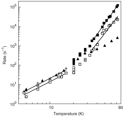

  

  The single-exponential rate constants (k₁ or 1/T₁) obtained by fitting the saturation-recovery transients of the UV-generated tyrosine radical (▴) are shown for the entire temperature range. The single-exponential rate constants obtained by fitting the saturation-recovery transients of the B2 tyrosyl radical (+) are shown for temperatures below 20 K. The saturation-recovery transients of the B2 tyrosyl radical were also fit with equations (7) and (8), where the first term in equation (8) was taken to be the dominant source of dipole–dipole-induced relaxation enhancement. The open squares (□) represent k_1i/k_1ex and the closed squares (▪) represent k_1d (ref. 4).

• 20 In the CW saturation-recovery experiment, the observe microwave power used to record the saturation-recovery transient can itself enhance the saturation-recovery rate, k₁. Because this enhancement is not orientation dependent, it affects only k_1i. The true value of k_1i, that is k_1i at zero power, can be determined as follows: record 3–4 saturation-recovery transients at the same temperature, but each at a different value of the observe power. Fit each saturation-recovery transient to the appropriate equation, a single exponential or equation (7), to determine k_1i(observe power 1), k_1i(observe power 2), etc. Plot k_1i versus observe power and extrapolate to zero power. Please note that this step is not required for the spin-echo-detected saturation-recovery experiment.

Collecting saturation-recovery transients of your protein sample

Timing 5 h

• 21 Insert the protein sample containing both the radical and paramagnetic metal center into the EPR cavity. Collect saturation-recovery transients over the temperature range described in Step 19. The length of the saturating pulse or pulse train should be ∼1/k_1i. This will be known if an appropriate control was available (see above), or one can determine it by fitting the data as it is collected. Alternatively, one can look at the saturation-recovery transient and determine where the curve reaches a plateau. This will be ∼5/k_1i. Note that the time required for each complete pulse sequence (the shot recovery time) should be 6/k_1i to allow complete recovery of all the radicals. It is better to overestimate the shot recovery time needed than to underestimate it.

Collecting saturation-recovery transients of the model system

Timing 5 h

• 22 Record saturation-recovery transients of your model system at the same temperatures as your protein sample. This allows direct calculation of the interspin distance, r, and direct comparison of the temperature dependence of k_1d in the two samples. For example, to measure the distance between the non-heme Fe(II) in PSII and its stable tyrosine radical Y_D^•, we used the photosynthetic reaction center from the purple non-sulfur bacterium Rhodobacter sphaeroides as a model system. This protein also contains a non-heme Fe(II) and the crystal structure was known⁴³. A stable cation radical, P⁺, 28 Å away from the non-heme Fe(II), was generated by illumination of the bacterial reaction center at low temperatures. Saturation-recovery transients of P⁺ were recorded and found to be non-single exponential (Fig. 7) as expected.

  Figure 7: Saturation-recovery transient from the radical P+ in the bacterial reaction center at 10 K.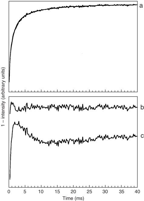

  

  In (a), the fit of equation (7) is shown superimposed on the data. In fitting the saturation-recovery transient, it was assumed that only the second term in equation (8) made a significant contribution to the relaxation enhancement. The value of k_1d from this fit was 3,500 s⁻¹. The observe microwave power level was 720 nW and the saturating microwave pulse (160 mW) was of 6-ms duration. The residual spectra (the difference between the saturation-recovery transient and the fitted curve) are shown on an expanded vertical scale for (b) equation (7) and (c) a single exponential. Note that a perfect fit to the data would yield a residual spectrum that was perfectly flat (horizontal), except for noise. Residual spectrum (b) shows that the fit of equation (7) comes close to this ideal. The inability of a single exponential to adequately fit the observe saturation-recovery transient of the radical, residual spectrum (c), is characteristic of the presence of a dipole–dipole interaction⁴⁶.

Data analysis

Timing 3 days

• 23 If your control sample is an appropriate model for determining k_1i, this rate constant can be extracted from single-exponential fits to the saturation-recovery data. At this time, no commercial programs set up to perform the fit described by equations (7) and (8) are known. However, fitting routines can be written within a number of commercial software packages, including Mathematica and MatLab.

• 24 In the absence of exchange coupling between the radical and the metal center, fit the data using equations (7) and (8) to obtain values for k_1i and k_1d. Use k_1d to calculate the distance between the radical and the metal center, as described above. Compare k_1i obtained from the protein sample to the k_1i of the control sample. If the values of k_1i determined from the protein sample are larger than k_1i from the control sample and the two differ in their temperature dependence, then it may be that an exchange coupling also exists between the radical and metal center in the protein. In this case, accurate determinations of both the exchange and dipole–dipole couplings will require an equation that incorporates both sources of relaxation enhancement into the fitting of the saturation-recovery transient²¹.

  Troubleshooting

Troubleshooting

Troubleshooting advice can be found in Table 1.

Table 1 Troubleshooting table.

Timing

Step 1: 1–2 h

Step 2: 30 min

Step 3: 30 min

Steps 4–8: 2 h

Steps 9 and 10: 2 h

Step 11: 2 h

Steps 12–20: 5 h

Step 21: 5 h

Step 22: 5 h

Steps 23 and 24: 3 days

Anticipated results

Comparison of k_1d arising from Fe(II) in PSII and Rb. sphaeroides reaction center

Both PSII and the bacterial reaction center from Rb. sphaeroides contain a non-heme Fe(II) coordinated by four histidine ligands. At the time of these experiments²⁶, the structure of the bacterial reaction center was known⁴³, allowing it to serve as a model system for PSII. In the bacterial reaction center, k_1d was extracted from fits of equation (7) to the spin–lattice relaxation transients of P⁺, the cation radical of the special pair. In PSII depleted of manganese, k_1d was extracted from fits of equation (7) to the spin–lattice relaxation transients of Y_D^•. The plot in Figure 8 shows that the temperature dependence of k_1d is the same in the two systems, indicating that the non-heme Fe(II) is the source of relaxation enhancement for both P⁺ and Y_D^•. The ratio of the dipolar rate constants in the two systems predicted a distance of 37 ± 5 Å between Y_D^• and the non-heme Fe(II) of PSII (equation (10)) (ref. 26). The x-ray crystal structure of PSII has since been solved at 3.5 Å (ref. 44) and 3.0 Å (ref. 45) resolution. These structures show a distance of 37 Å between Y_D^• and the non-heme Fe(II).

Figure 8: Plotting of the dipolar rate constants k_1d versus temperature for P⁺ (□), the cation radical of the special pair in photosynthetic reaction centers of Rb. sphaeroides, and for the tyrosine radical Y_D^• (▪) in Mn-depleted PSII. Since the P⁺–Fe(II) distance, r, is shorter than the Y_D^•–Fe(II) distance, the dipolar rate constant for P⁺ is greater at each temperature.

The lines show the best power law fit (k_1d = ATⁿ) for each set of rate constants²⁶. The fact that the dipolar rate constants for P⁺ and Y_D^• have the same temperature dependence is consistent with the non-heme Fe(II) being the source of relaxation enhancement in both the reaction center and Mn-depleted PSII.

Note: Supplementary information is available via the HTML version of this article.

References

Lakshmi, K. & Brudvig, G. Pulsed electron paramagnetic resonance methods for macromolecular structure determination. Curr. Opin. Struct. Biol. 11, 523–531 (2003).
Berliner L.J., Eaton G.R., & Eaton S.S. (eds.) Distance Measurements in Biological Systems by EPR (Kluwer Academic/Plenum Publishers, New York, 2000).
Hirsh, D.J., Beck, W.F., Innes, J.B. & Brudvig, G.W. Using saturation-recovery EPR to measure distances in proteins: applications to photosystem II. Biochemistry 31, 532–541 (1992).
Hirsh, D.J., Beck, W.F., Lynch, J.B., Que, L., Jr . & Brudvig, G.W. Using saturation-recovery EPR to measure exchange couplings in proteins: application to ribonucleotide reductase. J. Am. Chem. Soc. 114, 7475–7481 (1992).
MacArthur, R. et al. Component B binding to the soluble methane monooxygenase hydroxylase by saturation-recovery EPR spectroscopy of spin-labeled MMOB. J. Am. Chem. Soc. 124, 13392–13393 (2002).
Clegg, R.M. Fluorescence resonance energy transfer. in Fluorescence Imaging Spectroscopy and Microscopy Vol. 137 (eds. Wang, X.F. & Herman, B.) 179–251 (Wiley, New York, 1996).
Stryer, L. Fluorescence energy transfer as a spectroscopic ruler. Annu. Rev. Biochem. 47, 819–846 (1978).
Förster, T. Delocalized excitation and excitation transfer. in Modern Quantum Chemistry Vol. 3 (ed. Sinanoglu, O.) 93–137 (Academic Press Inc., New York, 1965).
Borbat, P.B. & Freed, J.H. Double-quantum ESR and distance measurements. in Distance Measurements in Biological Systems by EPR Vol. 19 (eds. Berliner, L.J., Eaton, G.R. & Eaton, S.S.) 383–456 (Kluwer Academic/Plenum Publishers, New York, 2000).
Raitsimring, A. “2 + 1” pulse sequence as applied for distance and spatial distribution measurements of paramagnetic centers. in Distance Measurements in Biological Systems by EPR Vol. 19 (eds. Berliner, L.J., Eaton, G.R. & Eaton, S.S.) 461–490 (Kluwer Academic/Plenum Publishers, New York, 2000).
Jeschke, G., Pannier, M. & Spiess, H.W. Distance measurements in biological systems by EPR. in Distance Measurements in Biological Systems by EPR Vol. 19 (eds. Berliner, L.J., Eaton, G.R. & Eaton, S.S.) 493–511 (Kluwer Academic/Plenum Publishers, New York, 2000).
Berliner L.J. (ed.) Spin Labeling 444 (Springer, New York, 2007).
Berliner L.J. (ed.) Spin Labeling II: Theory and Applications (Academic Press, New York, 1979).
Berliner L.J., (ed.) Spin Labelling 605 (Academic Press, New York, 1976).
Bloembergen, N. The interaction of nuclear spins in a crystalline lattice. Physica (The Hague) 15, 386–426 (1949).
Bloembergen, N., Purcell, E.M. & Pound, R.V. Relaxation effects in nuclear magnetic resonance absorption. Phys. Rev. 73, 679–712 (1948).
Bloembergen, N., Shapiro, S., Pershan, P.S. & Artman, J.O. Cross relaxation in spin systems. Phys. Rev. 114, 445–459 (1959).
Abragam, A. Overhauser effect in nonmetals. Phys. Rev. 98, 1729–35 (1955).
Kulikov, A.V. & Likhtenstein, G.I. Adv. Mol. Relax. Interact. Processes 10, 47–79 (1977).
Goodman, G. & Leigh, J.S. Jr. Distance between the visible copper and cytochrome a in bovine heart cytochrome oxidase. Biochemistry 24, 2310–2317 (1985).
Rakowsky, M., More, K., Kulikov, A., Eaton, G. & Eaton, S. Time-domain electron paramagnetic resonance as a probe of electron–electron spin–spin interaction in spin-labeled low-spin iron porphyrins. J. Am. Chem. Soc. 117, 2049–2057 (1995).
Eaton, G.R. & Eaton, S.S. Relaxation times of organic radicals and transition metal ions. in Distance Measurements in Biological Systems by EPR Vol. 19 (eds. Berliner, L.J., Eaton, G.R. & Eaton, S.S.) 29–154 (Kluwer Academic/Plenum Publishers, New York, 2000).
Debus, R.J., Feher, G. & Okamura, M.Y. Iron-depleted reaction centers from Rhodopseudomonas sphaeroides R-26.1: characterization and reconstitution with Fe2+, Mn2+, Co2+, Ni2+, Cu2+ and Zn2+. Biochemistry 25, 2276–2287 (1986).
Zhou, Y., Bowler, B., Lynch, K., Eaton, S. & Eaton, G. Interspin distances in spin-labeled metmyoglobin variants determined by saturation recovery EPR. Biophys. J. 79, 1039–1052 (2000).
Seiter, M., Budker, V., Du, J.-L., Eaton, G.R. & Eaton, S.S. Interspin distances determined by time domain EPR of spin-labeled high-spin methemoglobin. Inorg. Chim. Acta 273, 354–366 (1998).
Hirsh, D.J. & Brudvig, G.W. Long-range electron spin–spin interactions in the bacterial photosynthetic reaction center. J. Phys. Chem. 97, 13216–13222 (1993).
Portis, A.M. Electronic structure of F centers: saturation of the electron spin resonance. Phys. Rev. 91, 1071–1078 (1953).
Castner, T.G. Jr. Saturation of the paramagnetic resonance of a V center. Phys. Rev. 115, 1506–1515 (1959).
Galli, C., Innes, J., Hirsh, D. & Brudvig, G. Effects of dipole–dipole interactions on microwave progressive power saturation of radicals in proteins. J. Magn. Reson. B 110, 284–287 (1996).
Voss, J., Hubbell, W.L. & Kaback, H.R. Distance determination in proteins using designed metal ion binding sites and site-directed spin labeling: application to the lactose permease of Escherichia coli. Proc. Natl. Acad. Sci. USA 92, 12300–12303 (1995).
Roberts, J.D. ABCs of FT-NMR (University Science Books, Sausalito, CA, 2000).
Harris, R.K. Nuclear Magnetic Resonance Spectroscopy: A Physicochemical View (Wiley, New York, 1986).
Weil, J.A., Bolton, J.R. & Wertz, J.E. Electron Paramagnetic Resonance: Elementary Theory and Practical Applications 568 (Wiley, New York, 1994).
Symons, M.M.C. Chemical and Biochemical Aspects of Electron-Spin Resonance Spectroscopy 190 (John Wiley, New York, 1978).
Hyde, J.S., Swartz, H.M. & Antholine, W.E. in Spin Labeling II: Theory and Applications (ed. Berliner, L.J.) 71–113 (Academic Press, New York, 1979).
Hyde, J.S. Saturation recovery methodology. in Time-domain Electron Spin Resonance (eds. Kevan, L. & Schwartz, R.N.) 1–30 (Wiley, New York, 1979).
Yamauchi, T., Mino, H., Matsukawa, T., Kawamori, A. & Ono, T. Parallel polarization electron paramagnetic resonance studies of the S1-state manganese cluster in the photosynthetic oxygen-evolving system. Biochemistry 36, 7520–7526 (1997).
Bizzarri, A.R. & Cannistraro, S. Solvent modulation of the structural heterogeneity in FeIII myoglobin samples: a low temperature EPR investigation. Eur. Biophys. J. 22, 259–267 (1993).
Berthold, D.A., Babcock, G.T. & Yocum, C.F. A highly resolved, oxygen-evolving photosystem II preparation from spinach thylakoid membranes. FEBS Lett. 134, 231–234 (1981).
Pikal-Cleland, K.A., Rodriguez-Hornedo, N., Amidon, G.L. & Carpenter, J.F. Protein denaturation during freezing and thawing in phosphate buffer systems: monomeric and tetrameric beta-galactosidase. Arch. Biochem. Biophys. 384, 398–406 (2000).
Eaton, S.S. & Eaton, G.R. Irradiated fused-quartz standard sample for time-domain EPR. J. Magn. Reson. A 102, 354–356 (1993).
Sahlin, M. et al. Magnetic interaction between the tyrosyl free radical and the antiferromagnetically coupled iron center in ribonucleotide reductase. Biochemistry 26, 5541–5548 (1987).
Allen, J.P., Feher, G., Yeates, T.O., Komiya, H. & Rees, D.C. Structure of the reaction center from Rhodobacter sphaeroides R-26: protein–cofactor (quinones and Fe2+) interactions. Proc. Natl. Acad. Sci. USA 85, 8487–8491 (1988).
Ferreira, K.N., Iverson, T.M., Maghlaoui, K., Barber, J. & Iwata, S. Architecture of the photosynthetic oxygen-evolving center. Science 303, 1831–1838 (2004).
Loll, B., Kern, J., Saenger, W., Zouni, A. & Biesiadka, J. Towards complete cofactor arrangement in the 3.0 Å resolution structure of photosystem II. Nature (London, United Kingdom) 438, 1040–1044 (2005).
Hirsh, D.J. Using Saturation-recovery EPR to Measure Distances and Exchange Couplings in Proteins PhD thesis, Yale University (1993).
Du, J.-L., Eaton, G.R. & Eaton, S.S. Temperature, orientation, and solvent dependence of electron spin–lattice relaxation rates for nitroxyl radicals in glassy solvents and doped solids. J. Magn. Reson. A 115, 213–221 (1995).
Eaton, S.S. & Eaton, G.R. Determination of distances based on T1 and Tm effects. in Distance Measurements in Biological Systems by EPR Vol. 19 (eds. Berliner, L.J., Eaton, G.R. & Eaton, S.S.) 348–378 (Kluwer Academic/Plenum Publishers, New York, 2000).
Author information
Authors and Affiliations
Corresponding author
Ethics declarations
Competing interests
The authors declare no competing financial interests.
Supplementary information
Supplementary Fig. 1
Spectral diffusion in the inhomogeneously broadened EPR signal (PDF 80 kb)
Supplementary Discussion
Why saturation-recovery (and not inversion recovery)? (PDF 26 kb)
Rights and permissions
About this article
Cite this article
Hirsh, D., Brudvig, G. Measuring distances in proteins by saturation-recovery EPR. Nat Protoc 2, 1770–1781 (2007). https://doi.org/10.1038/nprot.2007.255
Published:
Issue Date:
DOI: https://doi.org/10.1038/nprot.2007.255
This article is cited by
-
Enhancement of Paramagnetic Relaxation by Photoexcited Gold Nanorods
Scientific Reports (2016)
Effect of Lanthanide and Cobalt Ions on Electron Spin Relaxation of Tempone in Glassy Water:Glycerol at 20 to 200 K
Applied Magnetic Resonance (2016)
Measuring Cu2+-Nitroxide Distances Using Double Electron–Electron Resonance and Saturation Recovery
Applied Magnetic Resonance (2013)
Comments
By submitting a comment you agree to abide by our Terms and Community Guidelines. If you find something abusive or that does not comply with our terms or guidelines please flag it as inappropriate.