
Abstract
This document explains some of the relevant methodological issues involved in planning a clinical study using survival and time-to-event outcome data, particularly in the field of haematopoietic stem cell transplantation, and indicates the appropriate statistical methods to use for the analysis. As the majority of these methods are commonly used in survival and event-history analysis, this document discusses their potential and limitations with reference to common SCT research situations. Some reference is given to methods, recently appearing in the literature that may be capable of handling complex investigations. These guidelines also address various practical issues, such as recoding or transforming variables in regression models or reporting results.
This is a preview of subscription content, access via your institution
Access options
Subscribe to this journal
Receive 12 print issues and online access
$259.00 per year
only $21.58 per issue
Buy this article
- Purchase on Springer Link
- Instant access to full article PDF
Prices may be subject to local taxes which are calculated during checkout


Notes
Other outcome variables in longitudinal studies, such as recurrent events or repeated measurements, are not common in current SCT research. Thus, we provide only one example of analysis in a situation characterised by multiple recurrences of relapse, which will be approached in the context of multi-state models (the analysis of current leukaemia-free survival). However, other statistical approaches may be more suitable in other situations. Methods for longitudinal data and for multivariate survival outcomes are not illustrated in these Guidelines. Even less common is analysing a continuous outcome variable, such as the level of WBC. Methods for the analysis of this type of outcome (t-test, analysis of variance, multiple regression and so on) can be found in any statistics textbook. A few are mentioned in Section 3.1.
EBMT internal guidelines for the conduct of studies are available for the investigators through the EBMT study offices.
This terminology might create some confusion for statisticians, as the perspective is ‘prospective’, that is, longitudinal. In statistics and epidemiology, the term ‘retrospective study’ is often used with a different meaning, as for example in the case–control study.
The discussion of these issues is beyond the scope of these Guidelines. EBMT adopts the ICH guidelines for the design of clinical trials.
In SCT trials, the comparison between treatments is usually made as parallel groups. In other settings, popular designs include the crossover, the factorial design and others.
In PCT comparing two or more treatments, randomisation, that is, the assignment of a patient to a treatment arm following a random process and independently of the patient's characteristics, is designed to (ideally) produce groups similar in terms of known and unknown risk factors. Blinding is adopted to reduce biased assessments of clinical responses.
A further ‘traditional’ possibility is a case-matched study, in which each patient from group A is matched to one or more patients from group B who are identical, or nearly so, with respect to one or more potential confounders. The analysis must apply specific methods for matched pairs. This method is more difficult to apply than the others, it is less efficient (using only a part of the available information) and it has less potential than regression methods for investigating the role of all possible confounders. Matching does have a function in the propensity score method (Section 4.4).
Recent literature proposes other approaches to the specific problem of removing potential confounding. In the context of the comparison of two treatment groups in a non-intention to treat non-randomised study (where, for example, propensity scores are used, Section 4.4), it is worth mentioning the use of adjusted survival curves.[42] This method uses inverse probability weights to create adjusted survival curves to artificially create comparable groups in terms of all factors that could have influenced the choice of treatment.
A different yet frequent goal of many studies is proposing a new risk score, or building a ‘good’ prognostic model for outcome prediction in general. Although this problem can also be approached using the methods described in this document (regression models), a proper investigation requires specific validation techniques whose illustration would be beyond the scope of these Guidelines. Throughout the document, we will identify issues such as this and suggest texts[28] that can be consulted that illustrate methods for assessing the predictive value of the model.
As indicated, the refinements of the study population (and of the statistical analysis plan) apply only (or especially) to RBS.
In a two-sided test, H1 states that there is a difference of whatever sign, positive or negative. A one-sided test fixes the sign of the expected difference.
Another important parameter whose meaning is worth recalling is the power (1−beta), which is the probability that the decision rule leads to ‘proving’ the presence of a difference that is actually present in the target population. Of course, this parameter should be high; it is, however, limited by the requirement of having a small alpha. The power is a key parameter in determining the sample size of a study.
What is described in this section is actually right-censoring, observations that are incomplete in the sense that, if we indicate with T the time to the event of interest, and with C the time to loss to follow-up, we have T>C. Situations with left- or interval-censoring are less common in practice, and the methods for addressing them become more complicated. Refer to Kalbfleisch and Prentice[43] (Section 3.2) for the theory on different patterns of censoring.
To be precise, this assumption can be slightly relaxed (see Kalbfleisch and Prentice[43]), but the substantial, interpretative meaning is the one reported here.
In this context, NRM is more appropriate than TRM, which stands for transplant-related mortality or, in non-transplant settings, treatment-related mortality, because TRM suggests classifying the cause of death as either transplant-related or not, while here we specifically mean ‘death without ever experiencing a prior relapse’. See also the remarks below in the ‘common mistakes’ subsection.
In fact, by NRM we mean mortality without prior relapse, and not mortality due to causes other than relapse.
Although it is customary to report these events in terms of simple percentages of occurrence and to neglect the competing events, this is often the wrong approach. Appropriate approaches are discussed in Section 2.2.3.
There is a semantic problem also for the event competing with relapse/progression: usually the acronym NRM is used, but more precisely we should use something like NRPM. In any case, it is important to specify (in presentations and in Statistical Methods sections) that we mean death without prior progression or relapse.
This is true unless the time between transplant and CR is included among the covariates.
This approach is also sometimes termed clock-forward, especially in the framework of multi-state models[5].
In practice, not all statistical software programs allow the researcher to apply left-truncation. With this approach, the survival data need to be arranged in the counting process form, that is, they must be represented as a triplet (entry time, final time and failure indicator).
The time threshold x should be chosen so that the most relevant part of the information is acquired by time x.
Recent statistical methods approach the estimation of the marginal survival function. Such efforts can be found in the work of Fine and others,[44] who introduced the term ‘semi-competing risks’ for settings where the role of two events is asymmetric, as it is here where death prevents relapse (‘truly competing’ events), but the converse is not true.
In statistics and epidemiology, ‘rate’ refers to a quantity that is not interpretable as a probability. However, in these Guidelines we follow the traditional practice of the medical literature and use this term to in fact mean ‘probability’.
An interesting example of grouped survival data is when it is not known precisely when the event occurred, but only that it occurred during a certain period, such as between two different scheduled follow-up times. Useful remarks can be found in the books by Kalbfleish and Prentice[43] and Marubini and Valsecchi.[2]
Standard deviations are usually computed applying the Greenwood formula. Note that the confidence intervals are obtained by neglecting the dependence between survival estimates at different times. For this reason, the band that connects the limits of the confidence intervals is not a proper confidence band for the whole curve. The R library km.ci implements several methods for computing pointwise confidence intervals as well as a ‘simultaneous’ confidence band.
The Gray test and the Fine and Gray regression model work best under the assumption of the proportionality of a mathematical quantity called the ‘sub-distribution hazard’, which unfortunately has no clinical meaning. This makes it difficult to determine when this hypothesis of proportionality may not occur; see for example Scheike and Zhang.[45]
An analysis of both CSH is efficaciously combined in a multi-state framework.
The ‘traditional’ separation of GVHD into acute and chronic based on a time threshold (100 days) is currently being replaced on a clinical basis, and as soon as data collection rises above this rigid definition, the statistical analysis will necessarily switch entirely to the competing risks setting. To date, acute GVHD was most often analysed as described in this section, while chronic GVHD as a competing risks endpoint was left-truncated (Section 2.1.4) at 100 days, thus restricting to survivors at 100 days.
The timing of engraftment, for example, would be described as the median among the cases who had engraftment.
Indicate with E1 the event of interest and with E2 the competing event. The corresponding probabilities of occurrence are π1 and π2; 1−π1−π2 represents the probability of being alive and failure-free (no event) at the time of assessment. Correspondingly, define:
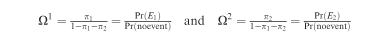
To compare two exposure groups, A and B, it is possible to implement regression models, where the effect of A vs B is estimated in terms of the ratios:
It was already remarked that censoring observations when the patients go off-protocol is erroneous (Section 2.1.1), and it is suggested in this case to define combined endpoints to account for interruptions or violations of the prescribed treatment, considering them as types of failure (Section 2.1.3).
We refer here to explanatory variables. Cases with a missing value for the main endpoints are usually excluded from the study, although the investigators should always be concerned with generalisation and bias (Section 2.3) and undertake the necessary investigations. A few missing values in secondary outcomes may be tolerated, but the reduction of the sample for that particular analysis must be documented in the publication, together with some discussion on whether the restricted population is still representative of the whole sample and whether there is any possible relationship between missing data and the value of the endpoint. The reasons are explained in the text.
In clinical trials, the presence of missing values for relevant variables is particularly problematic (for issues related to the ITT principle, see Section 2.3). The strategy used to manage missing values should always be indicated in the protocol of any type of prospective study. Avoiding missing values as much as possible should be planned for during any data collection or prospective study. Usually, it is necessary to restrict data collection to the main items needed, implement a good method of data entry, perform monitoring to avoid errors and so on.
This holds for X categorical covariates; if X is continuous, the best approach is to categorise it (in some texts, it is suggested instead to replace the missing value with a fixed value such as the mean or median of the known values of X, and add a dummy variable to indicate missing data (1 if missing, 0 if known) in the models (dummy variables are illustrated in Section 4.2.3).
The overall significance is tested using the Likelihood Ratio test. The Score test and the Wald test are based on approximations and generally lead to the same conclusions (if not, refer to the Likelihood Ratio test).
AIC=−2·Log-likelihood+kp, where p is the number of (relevant) parameters in the model, and k is a constant, usually 2. This quantity decreases as p begins to increase, up to the point where unnecessary variables are included. For its application in the framework of the Cox regression, see for example Klein and Moeschberger,17, par. 8.7.
The ‘forward’ approach adds the variables one after another, choosing the most significant at each step, until no variable adds significant information. The ‘backward’ procedure starts with all variables and removes the least significant variable at each step, until the loss of information becomes significant (between these two, the latter approach is preferred, unless the initial set is very large). Some software programs also implement combinations of forward and backward methods, or other methods (for example, ‘best subset’).
Interactions among more than two variables (typically three) can in principle be considered, but they hardly correspond to real biological phenomena. They are in any case very difficult to interpret, and thus are rarely seen.
To assess the presence of an interaction term X1*X2, the model must be ‘hierarchical’, that is, it must include both main effects X1 and X2.
Because it is a model of a hazard function, it can also be used to model the cause-specific hazard of an event with competing risks (Section 2.2.2).
In R this manipulation is necessary. Some libraries provide functions to do it, for example mstate or Epi. Continuous X(t) can be computed using the command survSplit from the in-built survival library.
Frailty models are extensions of the Cox regression to include random effects, represent unobserved heterogeneity or create dependence among observations from the same cluster, such as multiple endpoints for the same patient, or more simply observations from patients grouped according to the centre (to account for the centre effect). The latter situation can also be addressed with a ‘marginal’ approach that corrects the variance and covariance matrix (in R, see the options ‘frailty’ and ‘cluster’ within the coxph procedure, respectively).
This is also the context where adjusted survival curves[42] can be used, see note 8.
This idea is theoretically supported by work initiated by Rosenbaum and Rubin,[46] which shows that: (1) given the PS, the distribution of the covariates is the same in treated and not-treated groups, (2) under a condition called ‘strong ignorability’ (which corresponds to the assumption that there is no unmeasured confounder and that given the covariates there is no certainty regarding which treatment the patient will receive) and given a fixed PS, the difference of outcomes in treated and not-treated groups yields an unbiased estimate of the treatment effect.
For example, the standardised difference of two averages is:
 , where sj2 for j=0, 1 is the variance in group j.
The website provides the R software, general manuals, and other useful material or links. Additional programs for specific methods are available from local websites (R Cran). The programs (all documented with help files and a manual in pdf format) can be easily and quickly installed online or downloaded as archive files and then installed.


 , where sj2 for j=0, 1 is the variance in group j.
References
Bauer P . Multiple testing in clinical trials. Stat Med 1991; 10: 871–890.
Marubini E, Valsecchi MG . Analysing Survival Data from Clinical Trials and Observational Studies. Wiley: New York, 2004.
Beyersmann J, Gastmeier P, Wolkewitz M, Schumacher M . An easy mathematical proof showed that time-dependent bias inevitably leads to biased effect estimation. J Clin Epidemiol 2008; 61: 1216–1221.
Simon R, Makuch RW . A non-parametric graphical representation of the relationship between survival and the occurrence of an event: application to responder versus non-responder bias. Stat Med 1984; 3: 35–44.
Putter H, Fiocco M, Geskus RB . Tutorial in biostatistics: competing risks and multi-state models. Stat Med 2007; 26: 2389–2430.
Keiding N, Klein JP, Horowitz MM . Multi-state models and outcome prediction in bone marrow transplantation. Stat Med 2001; 20: 1871–1885.
Iacobelli S, Apperley J, Morris C . Assessment of the role of timing of second transplantation in multiple myeloma by multistate modeling. Exp Hematol 2008, 1567–1571.
Iacobelli S . Statistical modeling of complex disease histories in Bone Marrow Transplant. Guidelines for proper use and interpretation of the Cox model for the European Group for Blood and Marrow Transplantation. 2004. Available from the EBMT website www.ebmt.org.
van Houwelingen HC, Putter H . Dynamic predicting by landmarking as an alternative for multi-state modeling: an application to acute lymphoid leukemia data. Lifetime Data Anal 2008; 14: 447–463.
Klein JP, Rizzo JD, Zhang MJ, Keiding N . Statistical methods for the analysis and presentation of the results of bone marrow transplants. Part 1: Unadjusted analysis. Bone Marrow Transplant 2001; 28: 909–915.
Klein JP, Keiding N, Shu YY, Szydlo RM, Goldman JM . Summary curves for patients transplanted for chronic myeloid leukaemia salvaged by a donor lymphocyte infusion: the current leukaemia-free survival curve. Br J Haematol 2000; 109: 148–152.
Liu, Logan, Klein JP . Inference for current leukemia free survival. Lifetime Data Anal 2008; 14: 432–446.
Klein JP, Logan B, Harhoff M, Andersen PK . Analyzing survival curves at a fixed point in time. Stat Med 2007; 26: 4505–4519.
Logan B, Klein JP, Zhang MJ . Comparing treatments in the presence of crossing survival curves: an application to Bone Marrow Transplantation. Biometrics 2008; 64: 733–740.
Corbiere F, Joly P . A SAS macro for parametric and semiparametric mixture cure models. Comput Meth Programs Biomed 2007; 85: 173–180.
Sposto R . Cure model analysis in cancer: an application to data from the Children's Cancer Group. Stat Med 2002; 21: 293–312.
Klein JP, Moeschberger ML . Survival Analysis. Techniques for Censored and Truncated Data. 2nd edn. Springer: New York, 2003.
Therneau TM, Grambsch PM . Modeling Survival Data: Extending the Cox Model. Springer: Berlin, 2000.
Hosmer D, Lemeshow S, May S . Applied Survival Analysis: Regression Modeling of Time to Event Data, 2nd edn. Wiley: New York, 2008.
Gooley TA, Leisenring W, Crowley J, Storer BE . Estimation of failure probabilities in the presence of competing risks: new representation of old estimators. Stat Med 1999; 18: 695–706.
Gray RJ . A class of K-sample tests for comparing the cumulative incidence of a competing risk. Ann Stat 1988; 16: 1141–1154.
Fine JP, Gray RJ . A proportional hazard model for the subdistribution of a competing risk. JASA 1999; 94: 496–509.
Klein JP, Andersen PK . Regression modeling of competing risks data based on pseudo-values of the cumulative incidence function. Biometrics 2005; 61: 223–229.
Dignam JJ, Kocherginsky MN . Choice and interpretation of statistical tests used when competing risks are present. J Clin Oncol 2008; 26: 4027–4034.
Logan BR, Zhang MJ, Klein JP . Regression models for hazard rates versus cumulative incidence probabilities in haematopoietic cell transplantation data. Biol Bone Marrow Transplant 2006; 12 (Suppl 1): 107–112.
Latouche A. . Improving statistical analysis of prospective clinical trials in stem cell transplantation. An inventory of new approaches in survival analysis’. Technical Report of the CLINT—Establishment of infrastructure to support International Prospective Clinical Trials in Stem Cell Transplantation, 2010. Available from COBRA Preprint Series, Art. 70. http://biostats.bepress.com/cobra/ps/art70.
Klein JP . Modeling competing risks in cancer studies. Stat Med 2006; 25: 1015–1034.
Harrell Jr FE . Regression Modeling Strategies. Springer: Berlin, 2001.
Schemper M, Smith TL . A note on quantifying follow-up in studies of failure time. Control Clin Trials 1996; 17: 343–346.
Klein JP, Rizzo JD, Zhang MJ, Keiding N . Statistical methods for the analysis and presentation of the results of bone marrow transplants. Part 2: Regression modelling. Bone Marrow Transplantation 2001; 28: 1001–1011.
Andersen PK, Klein JP, Zhang MJ . Testing for centre effects in multi-centre survival studies: a Monte Carlo comparison of fixed and random effects tests. Stat Med 1999; 18: 1489–1500.
Glidden DV, Vittingho E . Modeling clustered survival data from multicentre clinical trials. Stat Med 2004; 23: 369–388.
Yamaguchi T, Ohashi Y, Matsuyama Y . Proportional hazards models with random effects to examine centre effects in multicentre cancer clinical trials. Stat Meth Med Res 2002; 11: 221–236.
Royston P, Altman DG, Sauerbrei W . Dichotomizing continuous predictors in multiple regression: a bad idea. Stat Med 2006; 25: 127–141.
Statistical Methods in Medical Research 1994 Vol. 3 (Five papers on frailty models for heterogeneity and dependence).
Scheike TH, Zhang MJ . Extensions and applications of the Cox-Aalen survival model. Biometrics 2003; 59: 1036–1045.
van Houwelingen HC . Dynamic prediction by landmarking in event history analysis. Scand J Stat 2007; 34: 70–85.
D’Agostino Jr RB . Tutorial in biostatistics. Propensity score methods for bias reduction in the comparison of a treatment to a non-randomized control group. Stat Med 1998; 17: 2265–2281.
Lunceford JK, Davidian M . Stratification and weighting via the propensity score in estimation of causal treatment effects: a comparative study. Stat Med 2004; 23: 2937–2960.
Senn S, Graf E, Caputo A . Stratification for the propensity score compared with linear regression techniques to assess the effect of treatment or exposure. Stat Med 2007; 26: 5529–5544.
Wei LJ, Glidden DV . An overview of statistical methods for multiple failure time data in clinical trials. Stat Med 1997; 16: 833–839.
Cole SR, Hernán MA . Adjusted survival curves with inverse probability weights. Comput Meth Prog Biomed 2004; 75: 45–49.
Kalbfleisch JD, Prentice RL . The Statistical Analysis of Failure Time Data. 2nd edn. Wiley: New York, 2002.
Fine JP, Jiang H, Chappell R . On semi-competing risks data. Biometrika. 2001; 88: 907–919.
Scheike TH, Zhang MJ . Flexible competing risks regression modeling and goodness-of-fit. Lifetime Data Anal 2008; 14: 464–483.
Rosenbaum PR, Rubin DB . The central role of the propensity score in observational studies for causal effect. Biometrika 1983; 70: 41–55.
Scrucca L, Santucci A, Aversa F . Competing risk analysis using R: an easy guide for clinicians. Bone Marrow Transplant 2007; 40: 381–387.
Scrucca L, Santucci A, Aversa F . Regression modeling of competing risk using R: an in depth guide for clinicians. Bone Marrow Transplant 2010; 45: 1388–1395.
de Wreede L, Fiocco M, Putter H . mstate. An R package for the analysis of competing risks and multi-state models. J Stat Softw 2011; 38: 1–30.
de Wreede L, Fiocco M, Putter H . The mstate package for estimation and prediction in non- and semi-parametric multi-state and competing risks models. Comput Meth Prog Biomed 2010; 99: 261–274.
Acknowledgements
L. de Wreede contributed to the final version. All members of the EBMT Statistical Committee reviewed the Guidelines and agreed with the final version. SI has received grant support through her research position at the Tor Vergata University of Rome.
Author information
Authors and Affiliations
Consortia
Ethics declarations
Competing interests
The author declares no conflict of interest.
Additional information
Statistical Committee: Myriam Labopin (Chair), Ariane Boumendil, Ronald Brand, Ulrike Poetschger, Antonella Santucci, Stefan Suciu, Richard Szydlo, Liesbeth de Wreede.
Sponsorship Statement: This supplement is sponsored by the European Group for Blood and Marrow Transplantation (EBMT).
Appendix
Appendix
Procedures/commands in R, SAS and SPSS
For the purpose of helping new users perform their analyses, we provide here a list of procedures and instructions for the methods indicated in the previous chapters that are available in the statistical software packages R, SAS and SPSS. These three software programs are very commonly used in clinical analysis, but other reliable programs may provide good tools for survival and event-history analysis, for example STATA.
R is a reliable software package that is distributed freely on the web (http://www.r-project.org).Footnote 49 Although it may appear difficult to use, we encourage investing some time and patience in learning how to use it, especially if the user is willing to apply more than the usual standard methods of survival analysis. Consider also that the majority of basic statistical procedures can be applied through a menu-based interface (R Commander, for which you will need to install the library Rcmdr), and that there is abundant material available to facilitate the use of this program.,
This list is not an exhaustive companion for statistical analysis; it is only intended to help new users quickly find material to start their search in the Help pages of the software.
Rights and permissions
About this article
Cite this article
Iacobelli, S., On behalf of the EBMT Statistical Committee. Suggestions on the use of statistical methodologies in studies of the European Group for Blood and Marrow Transplantation. Bone Marrow Transplant 48 (Suppl 1), S1–S37 (2013). https://doi.org/10.1038/bmt.2012.282
Published:
Issue Date:
DOI: https://doi.org/10.1038/bmt.2012.282
Keywords
This article is cited by
-
Artificial intelligence methods to estimate overall mortality and non-relapse mortality following allogeneic HCT in the modern era: an EBMT-TCWP study
Bone Marrow Transplantation (2024)
-
Treosulfan compared to busulfan in allogeneic haematopoietic stem cell transplantation for myelofibrosis: a registry-based study from the Chronic Malignancies Working Party of the EBMT
Bone Marrow Transplantation (2024)
-
Automating outcome analysis after stem cell transplantation: The YORT tool
Bone Marrow Transplantation (2023)
-
A convolutional neural network-based model that predicts acute graft-versus-host disease after allogeneic hematopoietic stem cell transplantation
Communications Medicine (2023)
-
Acute kidney injury in multiple myeloma patients undergoing autologous hematopoietic stem cell transplant: a cohort study
Journal of Nephrology (2023)
