Abstract
A cycle is the simplest structure that brings redundant paths in network connectivity and feedback effects in network dynamics. An in-depth understanding of which cycles are important and what role they play on network structure and dynamics, however, is still lacking. In this paper, we define the cycle number matrix, a matrix enclosing the information about cycles in a network, and the cycle ratio, an index that quantifies node importance. Experiments on real networks suggest that cycle ratio contains rich information in addition to well-known benchmark indices. For example, node rankings by cycle ratio are largely different from rankings by degree, H-index, and coreness, which are very similar indices. Numerical experiments on identifying vital nodes for network connectivity and synchronization and maximizing the early reach of spreading show that the cycle ratio performs overall better than other benchmarks. Finally, we highlight a significant difference between the distribution of shorter cycles in real and model networks. We believe our in-depth analyses on cycle structure may yield insights, metrics, models, and algorithms for network science.
Introduction
The last two decades have witnessed extensive development in network science (NS)1, with research focuses being shifted from discovering macroscopic properties2,3,4 to uncovering the functional roles played by microscopic structures, or even individual nodes and links5,6,7. Scientists have pieced an increasingly clear picture about the functions of specific structures in disparate dynamical processes, such as the roles of different motifs in biological and communication networks5, how information and behaviors propagate along a contacting chain8, and how a local star structure self-sustains an epidemic spreading process9,10.
Besides extensively studied chain and star structures, cycle is another ubiquitously observed structure11, which plays significant roles in both structural organization and functional implementation. A cycle, also called loop in literature, can be simply defined as a closed path with the same starting and ending node. Recent studies have uncovered the topological properties of cycles, including the distribution of cycles of different sizes in real and artificial networks12,13,14,15,16, the effect of degree correlations on the loops of scale-free networks17, as well as the significant roles of the cycles in network functions related to storage18, synchronizability19, and controllability20. Cycles are also used as a tool to measure the extent of network being close to tree networks, and thus a significant difference between model networks and real networks is found, that is, the former can’t accurately reproduce the cycle structure in the latter21. In addition, the organization of cycles can be utilized to characterize individual nodes and links. For example, a measure called clustering coefficient (also called local clustering coefficient)2 is based on counting the number of associated triangles (triangle is the cycle with smallest size), which recently considered the associated cycles with larger sizes11,22,23, and was extended to the higher order cases22 and the weighted cases24,25. The edge multiplicity measures the number of triangles passing through an edge26. The effect of the addition of a none-observed link on the local organization of cycles can be used to estimate the likelihood of the existence of this link27, and the probability a self-avoid random walker returns to the target node through a cycle (cycles with different lengths are assigned to different weights) can be used to quantify the importance of the target node28.
Considering a simple network where direction and weight of a link are ignored and self-loops are not allowed, then a cycle is the simplest structure providing redundant paths to all involved node pairs. That is to say, if two nodes belong to a cycle, there are at least two independent paths connecting them. Such redundancy also brings complicated feedbacks in interacting dynamics. Therefore, the in-depth understanding of cycle structure may provide insights and methods on how to maintain the network connectivity under attacks29, how to regulate interacting dynamics toward predesigned states30 and how to maximize the early reach of spreading in short time31.
In this paper, according to the cycle-based statistics, we propose a matrix (named cycle number matrix) to represent cycle information of network, and an index (named cycle ratio) to quantify the importance of individual nodes. This index is essentially different from well-known indices and methods7, producing a much different ranking of nodes comparing with degree3, H-index32, and coreness10. Extensive experiments on real networks in identifying the most vulnerable nodes under intentional attacks33,34, the most efficient nodes in pinning control35,36,37 and the most influential nodes in the early stage of epidemic spreading31,38 show that cycle ratio performs overall better than other benchmarks including degree, H-index, and coreness. Finally, we highlight a significant difference between the distribution of shorter cycles in real and model networks.
Results
Definition of cycle ratio
Considering a simple network \(G(V,E)\), where V and E are the sets of nodes and links, respectively. The size of a cycle equals the number of links it contains. The cycles containing node i with the smallest size are defined as node i’s associated shortest cycles (also called i’s shortest cycles for simplicity) and the corresponding size is called node i’s girth19. Denote by \(S_i\) the set of the shortest cycles associated with node i, and \({{{{{S}}}}} = \cup _{{{{{{i}}}}} \in V}S_{i}\) the set of all shortest cycles of G, we define the so-called cycle number matrix \(C = \left[ {c_{ij}} \right]_{N \times N}\) to characterize the cycle structure of G, where N=|V| is the number of nodes in G, and \(c_{ij}\) is the number of cycles in S that pass through both nodes i and j if \(i \ne j\). If \(i = j\), \(c_{ii}\) is the number of cycles in S that contain node i. Obviously, \(C\) is a symmetric matrix. Based on the cycle number matrix, we propose an index, named cycle ratio, to measure a node’s importance as
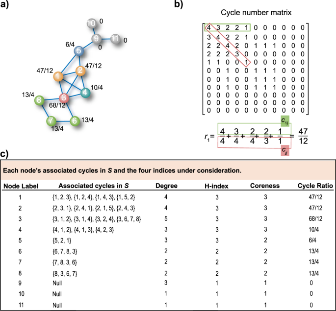
According to the above definition, if a node i doesn’t belong to any cycle in S, its cycle ratio is reasonably set to be zero. When \(c_{ii} > 0\), all items in the summation are well defined since \(c_{jj} > 0\) if \(c_{ij} > 0\). The ratio estimates the importance of node i subject to its participation to other nodes’ shortest cycles in S. Note that, in our definition, only shortest cycles associated with each node are considered since cycles with larger sizes are usually less relevant to the network functions (we have also tested on longer cycles, see details in Discussion) and to account for all cycles is infeasible for most networks due to the tremendous computational complexity27 (Supplementary Fig. 1 in Supplementary Note 1 shows the number of cycles with different lengths, indicating an exponential growth). Figure 1a presents an example network, and Fig. 1b shows the corresponding cycle number matrix. The process to calculate the cycle ratio of an example node (i.e., node 1) is also shown in Fig. 1b. In Eq. 1, each term represents the degree to which node i (i=1 for this example) participates in \(j\)’s associated shortest cycles (\(j = 1,2,3,4\,{{{{{{{\mathrm{and}}}}}}}}\,5\) for this example) in which denominator is the number of shortest cycles of node \(j\), and the numerator is the number of cycles associated with both node i and node \(j\). For example, the second term in the example equation in Fig. 1b, 3/4, means that three of the four shortest cycles of node 2 ({2, 3, 1}, {2, 4, 1}, {2, 1, 5}, {2, 4, 3}) contain node 1. In a word, \(r_1\) represents the degree to which node 1 participates in associated shortest cycles of other nodes. The cycle ratios of all nodes are presented in Fig. 1c. Three well-known node centralities, degree3, H-index32, and coreness10 (see precise definitions of these indices in Methods), are used as benchmarks for comparison. Their values for this example network are also presented in Fig. 1c.
a An example network with cycle ratios of nodes. Here the number in each node is its label, the value next to it is its cycle ratio and nodes of the same color have the same cycle ratio. b The cycle number matrix of example network in (a) and how to calculate the cycle ratio of node 1. Here the element \(c_{ij}\) in cycle number matrix is the number of shortest cycles that pass through both nodes \(i\) and \(j\) if \(i\, \ne\, j\). If \(i = j\), \(c_{ii}\) is the number of shortest cycles that contain node \(i\). For node 1 the non-zero elements in the green square in the matrix are neighbors with common shortest cycles with node 1, and each value (\(c_{1j}\), where \(j = 1,2,3,4\,{{{{{{{\mathrm{and}}}}}}}}\,5\)) represents the number of these cycles. The elements in the red square (\(c_{jj}\), where \(j = 1,2,3,4\,{{{{{{{\mathrm{and}}}}}}}}\,5\)) are the number of shortest cycles of each neighbor. The sum of the ratios of \(c_{1j}\) and \(c_{jj}\) is the cycle ratio of node 1. c Every node’s associated cycles in \(S\), degree, H-index, coreness10 and cycle ratio. Here \(S\) is the set of all shortest cycles of example network in (a) and \(S = \{ \{ 1,2,3\} ,\{ 1,2,4\} ,\{ 1,2,5\} ,\{ 1,3,4\} ,\{ 2,3,4\} ,\{ 3,6,7,8\} \}\).
Data
We test the performance of cycle ratio in identifying vital nodes subject to three well-studied dynamical processes, node percolation33,34, synchronization30, and epidemic spreading38. The first one considers nodes’ ability to maintain the network connectivity, the second one accounts for nodes’ capacity to regulate interacting dynamics toward a certain predesigned state, and the last one concentrates on infected nodes’ reach in the early stage of an epidemic outbreak. The experiments are carried out on six real networks from disparate fields, including the neural network of C. elegans (C. elegans)39, the email communication network of the University at Rovira i Virgili in Spain (Email)40, the collaboration network of jazz musicians (Jazz)41, the collaboration network of scientists working on NS42, the US air transportation network (USAir)32, and the protein-protein interaction network of yeast (Yeast)43. Their basic topological features are summarized in Table 1.
Correlation analysis
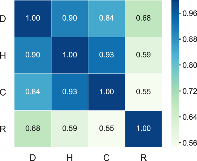
Before penetrating into each index’s ability to identify vital nodes, we first see whether cycle ratio contains rich information in addition to the three benchmarks. We apply the Kendall’s Tau (\(\tau\))44,45 to measure the correlation between pairs of indices (see the definition of \(\tau\) in Methods). Given two indices X and Y, if \(\tau (X,Y)\) is close to 1, it indicates that X and Y are highly correlated and less differential to each other. Figure 2 shows the average correlation matrix between all index pairs for the six networks (the correlation matrix for each network is shown in Supplementary Fig. 2 in Supplementary Note 2), one can clearly observe that the correlations between degree, H-index, and coreness are markedly high than the correlations between cycle ratio and the other three, the average of \(\tau\) over the six networks is 0.89 for the former and 0.61 for the latter. That is to say, the resulted node rankings produced by degree, H-index, and coreness are very similar to each other. Therefore, although the performance of H-index or coreness in some specific tasks is better than degree10,32, the node rankings produced by H-index and coreness contain less information in addition to the one produced by degree, and vice versa. In contrast, as suggested by the lower correlations, the node rankings produced by cycle ratio have rich information in addition to these produced by degree, H-index, and coreness. This is a very important yet easy-to-be-ignored marker about the potential value of the proposed index since the lower correlations between the proposed index and known indices indicate a higher possibility that the proposed index will provide insights beyond known indices. Besides, Supplementary Note 3 shows the distributions of the four indices for the six real networks under consideration. One can observe that the distinguishability of cycle ratio with most fractions is good while the distinguishability of coreness is poor.
Here D, H, C and R represent degree, H-index, coreness, and cycle ratio, respectively. Details of the six networks are shown in Table 1. Each element is the averaged value of the correlation \(\tau\) between the two indices corresponding to its position over the six networks, and the value is visualized by the color. See detailed calculation of the correlation \(\tau\) in Methods.
We are interested in comparing the difference between cycle ratio and local clustering coefficient which is the simplest index based on the neighborhood cycles. The local clustering coefficient of a node in network is the fraction of triangles that actually exist over all possible triangles in its neighborhood. In despite of the conceptual overlap, cycle ratio is largely different from local clustering coefficient in three aspects: (i) the considered shortest cycles (i.e., cycles in \(S\)) are not necessarily to be triangles; (ii) cycle ratio is not a local index since even node \(i\) and node j are distant in a network, the value of \(c_{ij}\) can be nonzero; (iii) cycle ratio is not a ratio but the sum of ratios, and thus its value can be greater than 1. Supplementary Note 4 compares the difference between cycle ratio and clustering coefficient in detail and shows that the correlations between clustering coefficient and the other four indices are the lowest. Although clustering coefficient can reflect the local connection, it cannot reflect the importance of a node. Notice that, due to the sparsity and hierarchical organization of many real networks, the local clustering coefficient is usually negatively correlated with degree (typically, local clustering coefficient scales as \(k^{ - 1}\))46,47, and thus not a good index for influential nodes. Similarly, Supplementary Fig. 12 in Supplementary Note 5 shows that the correlations between eigenvector centrality48 and the other four indices are low.
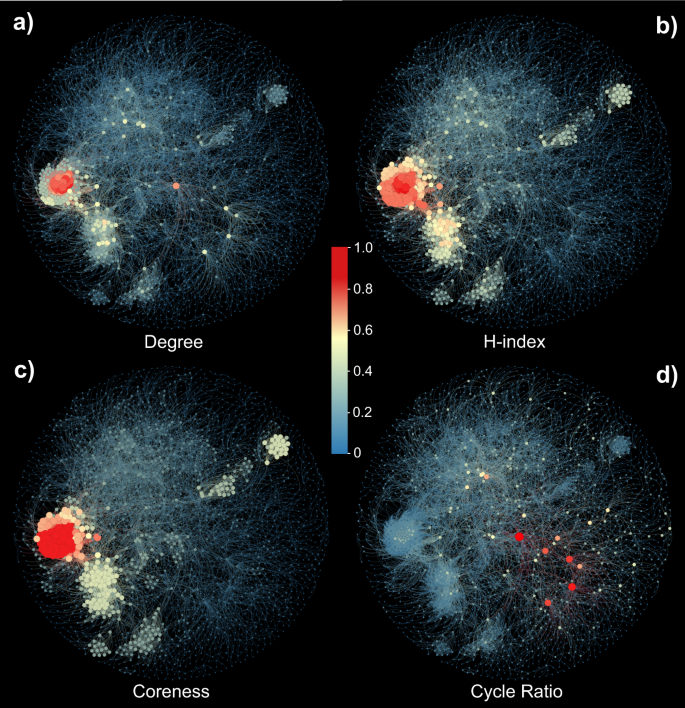
Figure 3 presents visualized Yeast network corresponding to the resulted rankings by the four indices. Very intuitively, the vital nodes selected by degree, H-index, and coreness are densely connected with each other and clustered in a certain region, in consistent to the so-called rich-club phenomenon49,50. As a contrast, the vital nodes selected by cycle ratio are scattered in the whole network with sparser connections among them. This is a significant advantage of cycle ratio if one would like to find out a set of vital nodes, because if the selected vital nodes tend to be clustered to each other, their influential areas will be highly overlapped and thus their collective influences are probably weaker10,51,52. Therefore, we believe the in-depth analyses of cycle ratio may uncover insights that cannot be directly obtained by other benchmark centralities.
The Yeast network is taken for example. In each plot, the sizes and colors of nodes are proportional to their relative values of the corresponding indices normalized by their respective maximum values. The position of each node in the four plots is fixed. For example, in (a), a node i’s relative value is \(k_i/k_{{{\mathrm{max}}}}\) where \(k_i\) is i’s degree and \(k_{{{\mathrm{max}}}}\) is the maximum degree of Yeast. Analogously, (b–d) show the results of H-index, coreness and cycle ratio, respectively. In (a–c), the vital nodes are densely connected with each other and clustered in several certain regions, and this effect increases in turn. In (d), however, the situation is completely different where the vital nodes scattered throughout the whole network.
Percolation
To evaluate the importance of nodes in maintaining the network connectivity, we study the node percolation dynamics33,34. Given a network, we remove one node at each time step and calculate the size of the largest component of the remaining network until the remaining network is empty. The metric called Robustness53 is used to measure the performance, defined as
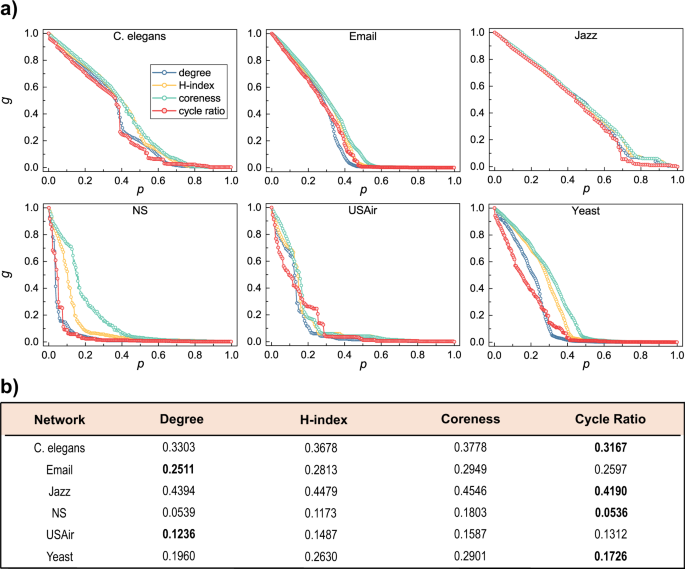
where the relative size \(g(n)\) is the number of nodes in the largest component divided by N after removing n nodes. The normalization factor 1/N ensures that the values of R of networks with different sizes can be compared. For each index, we compute once to get a fixed ranking of nodes. The node with largest index value is removed preferentially. Obviously, a smaller R means a quicker collapse and thus a better performance. Figure 4a shows the collapsing processes in the six real networks, resulted from the node removal by cycle ratio and the other three indices. For the majority of the considered networks, cycle ratio leads to much faster collapse than other indices. Figure 4b exhibits the Robustness R, from which one can see that the cycle ratio is overall the best index in identifying the most vital nodes in maintaining the network connectivity. In addition, Supplementary Figs. 10 and 13 in Supplementary Note 4 and Supplementary Note 5 respectively show the results of clustering coefficient and eigenvector centrality, respectively, and the same conclusion can be obtained.
a The \(x\)-axis denotes the ratio of removed nodes and the \(y\)-axis shows the relative size of the largest component after node removal. For each index, the node with the largest index value is removed each time and calculate the size of the largest component of the remaining network. b The robustness \(R\) of the four indices for the six real networks. For each network, best performed index with minimum robustness \(R\) is emphasized in bold.
Pinning control
We next evaluate the importance of nodes by measuring the effect caused by pinning these nodes in a synchronizing process35,36. Considering a general case where a simple connected network \(G\left( {V,E} \right)\) is consisted of N linearly and diffusively coupled nodes, with an interacting dynamics as
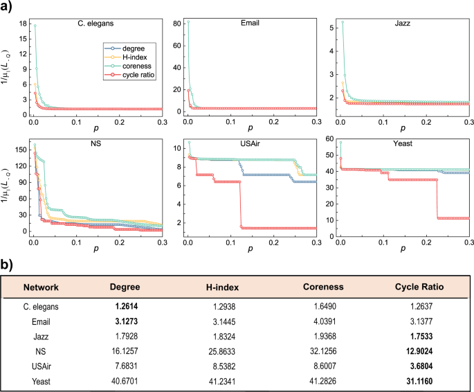
where the vector \(x_i \in {{{{{{{\mathbf{R}}}}}}}}^n\) is the state of node i, the function \(f( \cdot )\) describes the self-dynamics of a node, the positive constant \(\sigma\) denotes the coupling strength, Ui is the controller applied at node i, and the inner coupling matrix \({{\Gamma }}:{{{{{{{\mathbf{R}}}}}}}}^n \to {{{{{{{\mathbf{R}}}}}}}}^n\) is positive semidefinite. The Laplacian matrix \(L = [l_{ij}]_{N \times N}\) of G is defined as follows. If \((i,j) \in E\), then \(l_{ij} = - 1\); if \((i,j)\, \notin\, E\) and \(i\, \ne\, j\), then \(l_{ij} = 0\); if \(i = j\), then \(l_{ii} = - \mathop {\sum}\nolimits_{j \ne 1} {l_{ij}}\). The goal of pinning control is to drive the system from any initial state to the target state in finite time by pinning some selected nodes. Analogous to the node percolation, all nodes are ranked in the descending order by a given index. Then, we successively pin nodes one by one according to the ranking and quantify the synchronizability of the pinned networks, which can be measured by the reciprocal of the smallest nonzero eigenvalue of the principal submatrix54,55 (a smaller value corresponds to a higher synchronizability), namely \(1/\mu _1(L_{ - Q})\), where Q is the number of pinned nodes, \(L_{ - Q}\) is the principal submatrix, obtained by deleting the Q rows and columns corresponding to the Q pinned nodes from the original Laplacian matrix L, and \(\mu _1(L_{ - Q})\) is the smallest nonzero eigenvalue of \(L_{ - Q}\). Inspired by the metric Robustness, we propose a similar metric named pinning efficiency to characterize the performance of an index subject to pinning control, as
where \(Q_{{{\mathrm{max}}}}\) is the maximum number of pinned nodes under simulation. Here we set \(Q_{{{\mathrm{max}}}} = 0.3N\), and we have checked that the choices of \(Q_{{{\mathrm{max}}}}\) will not affect the conclusion. Figure 5a shows how \(1/\mu _1(L_{ - Q})\) decays with increasing number of pinned nodes. Obviously, a faster decay corresponds to a better performance. Figure 5b compares the pinning efficiency of the four indices. Similar to the result of the node percolation, cycle ratio is overall the best index in identifying the most efficient nodes in pinning control. In addition, Supplementary Tables 1 and 2 in Supplementary Note 4 and Supplementary Note 5 respectively show the results of clustering coefficient and eigenvector centrality and the same conclusion can be obtained.
a The x-axis denotes the ratio of pinned nodes and the \(y\)-axis shows network synchronizability after pinning the fraction of nodes. For each index, the nodes are pinned one by one in descending order of the index and quantify the synchronizability of the pinned networks each time. b The pinning efficiency \(P\) of the four indices for the six real-world networks. For each network, best performed index with minimum pinning efficiency \(P\) is emphasized in bold.
Epidemic spreading
Lastly, we consider the spreading dynamics. Since in viral marketing and online information transmission, people are more interested in maximizing the reach in short time, and in epidemiological control, the most critical issue is the spreading range and control measures in the early stage of outbreak (e.g., see the discussion of the efficacy of early control measures for COVID-1956,57, we concentrate on the fast influencers that play the dominant role in the early stage31. To quantify the influence of a set of selected nodes, we simulate the standard susceptible-infected-recovered (SIR) spreading dynamics38, where at each time step, each susceptible node will be infected by an infected neighbor with probability \(\beta\), and each infected node will be recovered with probability \(\gamma\). Initially, the top-0.1N nodes selected by each index are set to be infected and others are susceptible. The indices are ranked by cumulative infected nodes at a certain time step t, the more the better. We consider the case at \(\beta = \beta _c\) and \(\gamma = 1\), where
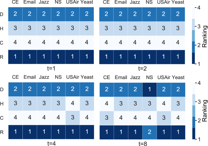
is the spreading threshold9,38 when \(\gamma = 1\). Here \(\langle k \rangle\) and \(\langle k^2 \rangle\) are the average degree and the average squared degree, respectively. Figure 6 reports the rankings of the four indices at time steps \(t = 1\), \(t = 2\), \(t = 4\) and \(t = 8\), where the values are averaged over 2000 independent runs. The best-performed index is ranked No. 1, the runner up is ranked No. 2, …, and the worst one is ranked No. 4. Among the 24 matches (i.e., 6 networks and 4 time steps), cycle ratio gets ranked No. 1 for 23 times and No. 2 for 1 time, it dramatically outperforms other indices. In addition, Supplementary Figs. 11 and 14 in Supplementary Note 4 and Supplementary Note 5 respectively show the results of clustering coefficient and eigenvector centrality and the same conclusion can be obtained. The results for more \(\left( {\beta ,t} \right)\) parameter sets are presented in Supplementary Note 6. In fact, the spreading capacity of cycle ratio is superior to coreness for both single-source and multiple-source cases, including fast spreading (considering the performance at the early stage) and complete spreading (see Supplementary Note 7).
Each matrix presents the results of the comparison of the four indices in a given time step of the spreading process. D, H, C and R represent degree, H-index, coreness, and cycle ratio, respectively. CE is the abbreviation of C. elegans. The elements in each matrix are the rankings of four indices at the corresponding time step, which is determined by cumulative infected nodes of each index in the SIR model simulation. The index with the largest number of infected nodes is ranked No. 1, and the others are ranked No. 2, 3, and 4 successively. Each ranking is averaged over 2000 independent runs and they are visualized by the color: the better the deeper. The infection probability is set as β = βc. for each network.
In addition to real networks, we have also analyzed two types of synthetic networks, the Erdős–Rényi (ER) networks58 and Barabási–Albert (BA) networks3. The overall performance of cycle ratio is just in the middle of the four indices. The reason for the not-so-good performance may be that the random networks are less localized (as indicated by the very small clustering coefficient) with lengths of shortest cycles (i.e., cycles in S) being relatively longer than real networks with similar sizes and densities (see Supplementary Note 8 and Supplementary Note 9), and thus effects of cycles on dynamical processes are weaker6,59.
Discussion
To represent cycle information of a network, this paper defines a matrix, called cycle number matrix, with which an index, called cycle ratio, can be calculated to quantify the importance of an individual node by simply measuring to which extent it is involved in other nodes’ associated shortest cycles. The basic idea underlying such an index is that if cycles are important in maintaining connectivity and interacting dynamics, then a node involved in many cycles should be vital. Experiments on real networks show that cycle ratio outperforms the other indices in identifying vital nodes that are critical in maintaining the network connectivity, efficient in pinning control and influential in epidemic spreading. In node percolation, it should be noted that the performance will be affected by dynamics itself in the way of greedy removal, so the removal order here is fixed as the result of the first calculation. Our finding thus has potential applicability in practice. For the node percolation, the top-ranked nodes should be firstly protected to maintain the network connectivity if there is a risk of functional loss of nodes. Reversely, if one would like to initiate an intentional attack, the top-ranked nodes are considered to be the primary targets. Such scenario is relevant to power grids60, air transportation networks, financial networks61, Internet, and so on62. Note that, when we consider an attack to an airport in the modern society, it does not mean we need to physically destroy it but disturb its information systems and signal systems. The critical nodes in pinning control can be pinned to efficiently approach the consensus of multiple agents63 and to ensure the coordination of unmanned aerial vehicles64 and mobile sensor networks65. Lastly, we proved cycle ratio is an efficient index for finding the susceptible individuals that need to be vaccinated in the early stage of epidemic spreading26,31.
It’s worth noting that the performance of cycle ratio is not necessarily better if longer cycles are considered. This is because when the longer cycles are counted, the difference in local cycle structure might be depressed. That is to say, the sets of associated cycles of many nodes will become more similar (i.e., with larger overlap), which may eventually lead to the decrease of the discriminability and thus the accuracy of the cycle ratio (see Supplementary Note 10).
An obvious insufficiency of cycle ratio is that it cannot be applied for trees or tree-like networks. Even for normal networks, a fraction of nodes may be not associated with any cycles. These nodes’ influences may be different but they are all assigned the same cycle ratio zero. One straightforward way to solve this issue is to combine cycle ratio with some other indices, for example, a mixed index could be \(r^ \ast = r_i + \varepsilon k_i\) with \(\varepsilon\) being a tunable parameter, hence all nodes with zero cycle ratio can be ranked by their degrees. Since cycle ratio and degree will produce markedly different rankings, a subtly designed combination of cycle ratio and degree has the potential to generate much better results than the single index. Similar improvement could also be achieved by combining cycle ratio with H-index or coreness. In contrast, the expected improvement by combining degree, H-index and coreness is lower since they are already very similar to each other. We leave this detailed problem for future study.
In addition, the method used to characterize the cycle structure can be extended to deal with hypernetworks66, where a hyperedge represents the interaction between multiple nodes. Treating hyperedges as the cycles in the set S and denoting \(\Omega\) the incidence matrix, whose element \(\Omega _{ie}\) indicates whether node i belongs to hyperedge e (\(\Omega _{ie} = 1\) indicates the belongness and \(\Omega _{ie} = 0\) otherwise), then we can obtain a matrix similar to the cycle number matrix by multiplying the incidence matrix by its transposed matrix, say \(\Omega \Omega ^T\), where the diagonal element [ΩΩT]ii represents the number of hyperedges involving node i and [ΩΩT]ij indicates the number of hyperedges that involving both node i and node j. Therefore, we can quantify a node’s importance in a hypernetwork by its participation to other nodes’ hyperedges.
We end this paper by presenting two open issues. Firstly, analogous to cycle ratio, one may also design cycle-based indices to quantify the likelihood of the existence of any unobserved link, which can find applications in solving the link prediction problem. Secondly, the good performance of cycle ratio, as well as the lower correlations between cycle ratio and other benchmark centralities, encourages the in-depth studies on cycle structure. In terms of global statistics, the model networks have lower average clustering coefficient and lower proximity to tree networks than real networks21; in terms of the distribution of shorter cycles, as shown in Supplementary Note 9, none of degree-preserved null model67, Watts–Strogatz model2 and Barabasi–Albert model3 can well reproduce the cycle-based statistics of real networks, indicating that the understanding about how cycles are formed may deepen our knowledge on the mechanisms underlying network organization. In addition to the shortest cycles, higher-order cycles also play important roles in network structure and functions68,69. Thus we expect to find more insights from spectral analysis of the cycle number matrix and analyzing longer and higher-order cycles in the future with the help of methodologies from algebraic topology69,70 and sufficient computational resource, and extend the findings and scope of applications reported in this paper.
Methods
Degree, H-index and Coreness
Degree of a node is the number of its immediate neighbors. H-index of a node i is the maximum integer h such that there are at least h neighbors of node i with degrees no less than h. Coreness is obtained by the k-core decomposition10. The k-core decomposition process starts by removing all nodes with degree \(k = 1\). This may cause new nodes with degree \(k \le 1\) to appear. These are also removed and the process stops when all remaining nodes are of degree \(k\, > \,1\). The removed nodes and their associated links form the 1-shell, and the nodes in the 1-shell are assigned a coreness value 1. This pruning process is repeated to extract the two-shell, that is, in each step the nodes with degree \(k \le 2\) are removed. Nodes in the two-shell are assigned a coreness value 2. The process is continued until all higher-layer shells have been identified and all nodes have been removed. In the literature, coreness is also referred to as k-shell index10.
Kendall’s Tau
We consider any two indices associated with all N nodes, \(X = (x_1,x_2, \ldots ,x_N)\) and \(Y = (y_1,y_2, \ldots ,y_N)\), as well as the N two-tuples \(( {x_1,y_1} ),( {x_2,y_2} ), \ldots ,(x_N,y_N)\). Any pair \(( {x_i,y_i} )\) and \(( {x_j,y_j} )\) are concordant if the ranks for both elements agree, namely if both \(x_i \, > \,x_j\) and \(y_i > y_j\) or if both \(x_i < x_j\) and \(y_i < y_j\). They are discordant if \(x_i > x_j\) and \(y_i < y_j\) or if \(x_i < x_j\) and \(y_i > y_j\). Here \(n_ +\) and \(n_ -\) are used to represent the number of concordant and discordant pairs, respectively. In addition, \(t_X\) is the number of the pairs in which \(x_i = x_j\) and \(y_i \ne y_j\), and \(t_Y\) is the number of the pairs in which \(x_i \, \ne \,x_j\) and \(y_i = y_j\). Notice that if \(x_i = x_j\) and \(y_i = y_j\), the pair is not added to either \(t_X\) or \(t_Y\). Comparing all \(N(N - 1)/2\) pairs of two-tuples, the Kendall’s Tau is defined as44
If X and Y are independent, \(\tau\) should be close to zero, and thus the extent to which τ exceeds zero indicates the strength of correlation. The above definition of Kendall’s Tau44 is an improved version of the original definition45, specifically designed to deal with the case with many equivalent elements.
Code availability
The custom code that supports the findings of this study is available at the following github repository: https://github.com/ftl129/CycleRatio.
References
Newman, M. E. J. Networks. Oxford Univ. Press (2018).
Watts, D. J. & Strogatz, S. H. Collective dynamics of ‘small-world’ networks. Nature 393, 440–442 (1998).
Barabási, A.-L. & Albert, R. Emergence of scaling in random networks. Sci. (80) 286, 509–512 (1999).
Newman, M. E. J. Assortative mixing in networks. Phys. Rev. Lett. 89, 208701 (2002).
Alon, U. Network motifs: theory and experimental approaches. Nat. Rev. Genet. 8, 450–461 (2007).
Lü, L. & Zhou, T. Link prediction in complex networks: a survey. Phys. A 390, 1151–1170 (2011).
Lü, L. et al. Vital nodes identification in complex networks. Phys. Rep. 650, 1–63 (2016).
Christakis, N. A. & Fowler, J. H. The spread of obesity in a large social network over 32 years. N. Engl. J. Med. 357, 370–379 (2007).
Castellano, C. & Pastor-Satorras, R. Thresholds for epidemic spreading in networks. Phys. Rev. Lett. 105, 218701 (2010).
Kitsak, M. et al. Identification of influential spreaders in complex networks. Nat. Phys. 6, 888–893 (2010).
Kim, H.-J. & Kim, J. M. Cyclic topology in complex networks. Phys. Rev. E 72, 036109 (2005).
Bianconi, G. & Capocci, A. Number of loops of size h in growing scale-free networks. Phys. Rev. Lett. 90, 078701 (2003).
Bianconi, G., Caldarelli, G. & Capocci, A. Loops structure of the Internet at the autonomous system level. Phys. Rev. E 71, 11–14 (2005).
Bianconi, G., Gulbahce, N. & Motter, A. E. Local structure of directed networks. Phys. Rev. Lett. 100, 118701 (2008).
Rozenfeld, H. D., Kirk, J. E., Bollt, E. M. & Ben-Avraham, D. Statistics of cycles: How loopy is your network? J. Phys. A. Math. Gen. 38, 4589–4595 (2005).
Bonneau, H., Hassid, A., Biham, O., Kühn, R. & Katzav, E. Distribution of shortest cycle lengths in random networks. Phys. Rev. E 96, 062307 (2017).
Bianconi, G. & Marsili, M. Effect of degree correlations on the loop structure of scale-free networks. Phys. Rev. E 73, 066127 (2006).
Lizier, J. T., Atay, F. M. & Jost, J. Information storage, loop motifs, and clustered structure in complex networks. Phys. Rev. E 86, 026110 (2012).
Shi, D., Chen, G., Thong, W. W. K. & Yan, X. Searching for optimal network topology with best possible synchronizability. IEEE Circuits Syst. Mag. 13, 66–75 (2013).
Ruths, J. & Ruths, D. Control profiles of complex networks. Sci. (80) 343, 1373–1376 (2014).
Zhang, W., Li, W. & Deng, W. The characteristics of cycle-nodes-ratio and its application to network classification. Commun. Nonlinear Sci. Numer. Simul. 99, 105804 (2021).
Fronczak, A., Hołst, J. A., Jedynak, M. & Sienkiewicz, J. Higher order clustering coeffcients in Barabási-Albert networks. Phys. A 316, 688–694 (2002).
Caldarelli, G., Pastor-Satorras, R. & Vespignani, A. Structure of cycles and local ordering in complex networks. Eur. Phys. J. B 38, 183–186 (2004).
Barrat, A., Barthélemy, M., Pastor-Satorras, R. & Vespignani, A. The architecture of complex weighted networks. Proc. Natl Acad. Sci. 101, 3747–3752 (2004).
Saramäki, J., Kivelä, M., Onnela, J. P., Kaski, K. & Kertész, J. Generalizations of the clustering coefficient to weighted complex networks. Phys. Rev. E 75, 2–5 (2007).
Pei, S. & Makse, H. A. Spreading dynamics in complex networks. J. Stat. Mech. Theory Exp. 2013, P12002 (2013).
Pan, L., Zhou, T., Lü, L. & Hu, C. K. Predicting missing links and identifying spurious links via likelihood analysis. Sci. Rep. 6, 22955 (2016).
Van Kerrebroeck, V. & Marinari, E. Ranking vertices or edges of a network by loops: a new approach. Phys. Rev. Lett. 101, 1–4 (2008).
Albert, R., Jeong, H. & Barabási, A.-L. Error and attack tolerance of complex networks. Nature 406, 378–382 (2000).
Arenas, A., Díaz-Guilera, A., Kurths, J., Moreno, Y. & Zhou, C. Synchronization in complex networks. Phys. Rep. 469, 93–137 (2008).
Zhou, F., Lü, L. & Mariani, M. S. Fast influencers in complex networks. Commun. Nonlinear Sci. Numer. Simul. 74, 69–83 (2019).
Lü, L., Zhou, T., Zhang, Q. M. & Stanley, H. E. The H-index of a network node and its relation to degree and coreness. Nat. Commun. 7, 10168 (2016).
Callaway, D. S., Newman, M. E. J., Strogatz, S. H. & Watts, D. J. Network robustness and fragility: Percolation on random graphs. Phys. Rev. Lett. 85, 5468–5471 (2000).
Cohen, R., Erez, K., Ben-Avraham, D. & Havlin, S. Breakdown of the internet under intentional attack. Phys. Rev. Lett. 86, 3682–3685 (2001).
Wang, X. F. & Chen, G. Pinning control of scale-free dynamical networks. Phys. A 310, 521–531 (2001).
Li, X., Wang, X. & Chen, G. Pinning a complex dynamical network to its equilibrium. IEEE Trans. Circuits Syst. I 51, 2074–2087 (2004).
Qiu, Z., Fan, T., Li, M. & Lü, L. Identifying vital nodes by Achlioptas process. N. J. Phys. 23, 033036 (2021).
Pastor-Satorras, R., Castellano, C., Van Mieghem, P. & Vespignani, A. Epidemic processes in complex networks. Rev. Mod. Phys. 87, 925–979 (2015).
Rossi, R. A. & Ahmed, N. K. The Network Data Repository with Interactive Graph Analytics and Visualization. In Twenty-Ninth AAAI Conference on Artificial Intelligence 4292–4293 (AAAI Press, 2015).
Guimerà, R., Danon, L., Díaz-Guilera, A., Giralt, F. & Arenas, A. Self-similar community structure in a network of human interactions. Phys. Rev. E 68, 065103 (2003).
Gleiser, P. M. & Danon, L. Community structure in jazz. Adv. Complex Syst. 06, 565–573 (2003).
Newman, M. E. J. Finding community structure in networks using the eigenvectors of matrices. Phys. Rev. E 74, 036104 (2006).
Jeong, H., Mason, S. P., Barabási, A. L. & Oltvai, Z. N. Lethality and centrality in protein networks. Nature 411, 41–42 (2001).
Knight, W. R. A computer method for calculating Kendall’s tau with ungrouped data. J. Am. Stat. Assoc. 61, 436–439 (1966).
Kendall, M. G. A new measure of rank correlation. Biometrika 30, 81–93 (1938).
Ravasz, E. & Barabási, A.-L. Hierarchical organization in complex networks. Phys. Rev. E 67, 026112 (2003).
Zhou, T., Yan, G. & Wang, B.-H. Maximal planar networks with large clustering coefficient and power-law degree distribution. Phys. Rev. E 71, 046141 (2005).
Bonacich, P. Factoring and weighting approaches to status scores and clique identification. J. Math. Sociol. 2, 113–120 (1972).
Zhou, S. & Mondragón, R. J. The rich-club phenomenon in the internet topology. IEEE Commun. Lett. 8, 180–182 (2004).
Colizza, V., Flammini, A., Serrano, M. A. & Vespignani, A. Detecting rich-club ordering in complex networks. Nat. Phys. 2, 110–115 (2006).
Zhang, J. X., Chen, D. B., Dong, Q. & Zhao, Z. D. Identifying a set of influential spreaders in complex networks. Sci. Rep. 6, 1–10 (2016).
Ji, S., Lü, L., Yeung, C. H. & Hu, Y. Effective spreading from multiple leaders identified by percolation in the susceptible-infected-recovered (SIR) model. N. J. Phys. 19, 073020 (2017).
Schneider, C. M., Moreira, A. A., Andrade, J. S., Havlin, S. & Herrmann, H. J. Mitigation of malicious attacks on networks. Proc. Natl Acad. Sci. 108, 3838–3841 (2011).
Liu, H., Xu, X., Lu, J. A., Chen, G. & Zeng, Z. Optimizing pinning control of complex dynamical networks based on spectral properties of grounded Laplacian matrices. IEEE Trans. Syst. Man, Cybern. Syst. 51, 786–796 (2018).
Pirani, M. & Sundaram, S. On the smallest eigenvalue of grounded Laplacian matrices. IEEE Trans. Autom. Contr. 61, 509–514 (2016).
Liu, Q.-H. et al. The COVID-19 outbreak in Sichuan, China: Epidemiology and impact of interventions. PLOS Comput. Biol. 16, e1008467 (2020).
Chen, D. & Zhou, T. Evaluating the effect of Chinese control measures on COVID-19 via temporal reproduction number estimation. PLoS ONE 16, e0246715 (2021).
Erdős, P. & Rényi, A. On the evolution of random graphs. Publ. Math. Inst. Hungarian Acad. Sci. 5, 17–60 (1960).
Katz, L. A new status index derived from sociometric analysis. Psychometrika 18, 39–43 (1953).
Albert, R., Albert, I. & Nakarado, G. L. Structural vulnerability of the North American power grid. Phys. Rev. E 69, 025103 (2004).
Haldane, A. G. & May, R. M. Systemic risk in banking ecosystems. Nature 469, 351–355 (2011).
Li, M. et al. Percolation on complex networks: theory and application. Phys. Rep. 907, 1–68 (2021).
Chen, F., Chen, Z., Xiang, L., Liu, Z. & Yuan, Z. Reaching a consensus via pinning control. Automatica 45, 1215–1220 (2009).
Tang, Y., Gao, H., Kurths, J. & Fang, J. A. Evolutionary pinning control and its application in UAV coordination. IEEE Trans. Ind. Inform. 8, 828–838 (2012).
Ögren, P., Fiorelli, E. & Leonard, N. E. Cooperative control of mobile sensor networks: adaptive gradient climbing in a distributed environment. IEEE Trans. Autom. Contr. 49, 1292–1302 (2004).
Suo, Q., Guo, J. L. & Shen, A. Z. Information spreading dynamics in hypernetworks. Phys. A Stat. Mech. its Appl 495, 475–487 (2018).
Maslov, S. & Sneppen, K. Specificity and stability in topology of protein networks. Sci. (80) 296, 910–913 (2002).
Sizemore, A. E. et al. Cliques and cavities in the human connectome. J. Comput. Neurosci. 44, 115–145 (2017).
Shi, D., Lü, L. & Chen, G. Totally homogeneous networks. Natl Sci. Rev. 6, 962–969 (2019).
Mahadevan, P., Krioukov, D., Fall, K. & Vahdat, A. Systematic topology analysis and generation using degree correlations. Comput. Commun. Rev. 36, 135–146 (2006).
Acknowledgements
This work is supported by the National Natural Science Foundation of China (Nos. 11622538, 61673150, 61433014, 11975071), and the Zhejiang Provincial Natural Science Foundation of China (No. LR16A050001). L.L. and T.Z. acknowledges the Science Strength Promotion Programme of UESTC.
Author information
Authors and Affiliations
Contributions
T.F., L.L., and D.S. conceived the idea and designed the experiments and T.Z. provided a complement to the design. T.F. and L.L. performed the research. All authors analyzed the data. T.F., L.L., and T.Z. wrote the paper. D.S. edited this paper. All authors discussed the results and reviewed the paper.
Corresponding authors
Ethics declarations
Competing interests
The authors declare no competing interests.
Peer review information
Communications Physics thanks Yanqing Hu and the other, anonymous, reviewer(s) for their contribution to the peer review of this work.
Additional information
Publisher’s note Springer Nature remains neutral with regard to jurisdictional claims in published maps and institutional affiliations.
Supplementary information
Rights and permissions
Open Access This article is licensed under a Creative Commons Attribution 4.0 International License, which permits use, sharing, adaptation, distribution and reproduction in any medium or format, as long as you give appropriate credit to the original author(s) and the source, provide a link to the Creative Commons license, and indicate if changes were made. The images or other third party material in this article are included in the article’s Creative Commons license, unless indicated otherwise in a credit line to the material. If material is not included in the article’s Creative Commons license and your intended use is not permitted by statutory regulation or exceeds the permitted use, you will need to obtain permission directly from the copyright holder. To view a copy of this license, visit http://creativecommons.org/licenses/by/4.0/.
About this article
Cite this article
Fan, T., Lü, L., Shi, D. et al. Characterizing cycle structure in complex networks. Commun Phys 4, 272 (2021). https://doi.org/10.1038/s42005-021-00781-3
Received:
Accepted:
Published:
DOI: https://doi.org/10.1038/s42005-021-00781-3
This article is cited by
-
Identifying key players in complex networks via network entanglement
Communications Physics (2024)
-
Central node identification via weighted kernel density estimation
Data Mining and Knowledge Discovery (2024)
-
Identifying Station Importance in Urban Rail Transit Networks Using a Combination of Centrality and Time Reliability Measures: A Case Study in Beijing, China
Urban Rail Transit (2024)
-
Cost effective approach to identify multiple influential spreaders based on the cycle structure in networks
Science China Information Sciences (2023)
-
Optimizing higher-order network topology for synchronization of coupled phase oscillators
Communications Physics (2022)
Comments
By submitting a comment you agree to abide by our Terms and Community Guidelines. If you find something abusive or that does not comply with our terms or guidelines please flag it as inappropriate.

