
Abstract
Earthquake precursory processes have been central to scientific inquiry for nearly a century. Recent advancements in earthquake monitoring, geodesy, and data analysis including artificial intelligence, have substantially improved our understanding of how earthquake sequences unfold leading to the mainshock. We examine the available seismological and geodetic evidence describing preparatory processes in 33 earthquake sequences with MW [3.2–9.0] across different tectonic and stress conditions. Our analysis reveals common patterns, and sheds light on the interplay of structural, tectonic and other boundary conditions that influence the dynamics of earthquake sequences, and hence, in the seismo-geodetic observables prior to the mainshock. We place particular emphasis on connecting observed phenomena to the underlying physical processes driving the sequences. From our findings, we propose a conceptual framework viewing earthquake preparation as a process involving several juxtaposed driving physical mechanisms on different temporal and spatial scales, jointly leading to the stress increase in the future epicenter.
Introduction
A persistent goal in geosciences is to enhance protection against seismic hazard. To advance this topic, scientists are working to understand whether hazardous earthquakes exhibit some characteristic process, either at short or long spatiotemporal scale, prior to the mainshock1,2,3,4. Ideally, if such processes could be reliably and systematically observed prior to large earthquakes, automated near-real-time data workflows could enable extended warning times. However, detecting earthquake preparation processes, and understanding their significance remains a challenge in seismology. The current state of knowledge reveals a diverse set of observations, including sequences with no detectable preparatory processes. The tectonic conditions that facilitate or impede detectable preparatory processes before mainshocks are still not well understood3,5. Overall, various lines of research suggest that the prospect of short-term earthquake prediction, if achievable, remains a goal for the future of seismology3,6.
The fundamental physical and mechanical processes that lead to earthquake preparation and nucleation have been studied both theoretically and experimentally. In the laboratory, early work in the 1980’s already achieved the observation of pre-failure processes7,8. These observations were supported by early fracture mechanics models9, which then evolved into widely accepted theoretical earthquake nucleation models, such as the slip-weakening9 and the rate-and-state10,11 models. These models predict a quasi-static phase of deformation prior to earthquakes, during which the initially stable slip in the future plane begins to accelerate (pre-slip). This pre-slip continues until a critical nucleation size, characterized by a crack length \({L}_{C}\), is reached10,12. At LC, the system becomes unstable and the rupture grows quasi-dynamically, i.e., an earthquake is initiated. A primary focus of these models and laboratory experiments has been to investigate the effect of stress and material heterogeneity within the pre-slip region in order to understand the occurrence of foreshocks12. These heterogeneities included structural fault properties such as roughness13,14,15,16, loading rate variation17, effective confining pressure18, normal stress19,20, fault strength21, temperature or the presence of fluids22,23,24. Another important focus has been to obtain direct observations of the microscale damage evolution during fault nucleation and propagation, and how they vary with respect to different properties, as for example rock type and stress25. A summary of the properties and processes that have been suggested to influence the preparation and nucleation of earthquakes is given in Box 1.
While laboratory earthquakes are, to some extent, understood, our comprehension of the processes leading to an earthquake in real faults is less clear26,27,28,29,30,31. To date, the upscaling of physical models and observations from the lab to nature remains a challenge. This is mainly due to the inherent complexity of major faults, and to our incomplete understanding of the physical processes that cause earthquakes in nature. In addition, the geophysical data available to characterize many earthquakes are limited and heterogeneous, especially when they occur in remote locations. As a result, many studies based on geophysical data show only sparse observations of the processes occurring prior to earthquakes, often leading to ambiguous interpretations of their preparatory processes (see e.g., the different mechanisms proposed for the 1999 MW 7.6 Izmit earthquake29,32, or discussion in Gomberg5.
In this study, we undertake a comprehensive review of numerous studies that analyzed geophysical data to shed light on the collective patterns and physical processes influencing the occurrence of earthquakes in nature. Our analysis shows that (1) there is a multitude of processes that can lead to a stress increment on faults, eventually triggering an earthquake, and (2) these physical processes can occur concurrently at spatial and temporal scales spanning several orders. To facilitate the reader’s understanding, we provide a Glossary of Terms that defines the nomenclature throughout the text (Box S1).
Models describing earthquake preparation and nucleation
A combination of laboratory, field and theoretical studies led to the formulation of two end-member models of earthquake nucleation, which predict the spatial and temporal evolution of stress and strength in the vicinity of a mainshock. These models have been widely used to describe the geophysical observations prior to an earthquake and are summarized as follows.
-
(1)
The pre-slip model predicts aseismic slip acceleration prior to an earthquake. The aseismic acceleration takes place within the nucleation zone, which increases in size until it reaches a critical nucleation length (LC), from which the earthquake dynamic rupture begins12 (Fig. 1a). It can be seen as a self-nucleation model, where the eventual observation of pre-slip indicates in advance that an earthquake will occur. Therefore, this model is compatible with earthquake predictability33,34. One outcome of this model is a scaling between the space occupied by foreshocks and the size of the incipient mainshock27,35,36. Precursory aseismic acceleration has been observed in the laboratory13 and in numerical models12. Experimentally, results consistent with this model have been observed in frictional rock deformation experiments on m-scale granite blocks with smooth faults performed at very low normal stress20. If present, aseismic pre-slip is expected to occur within the nucleation region of the future dynamic rupture, with the slip release accelerating as dynamic rupture approaches. In nature, however, there are almost no observations of earthquake mainshocks preceded by well-documented aseismic or slow deformation that unambiguously represents pre-slip. Earthquake sequences from tectonic environments such as oceanic transform faults, where aseismic deformation accommodates a substantial proportion of the plate movement, have been proposed to be particularly consistent with the pre-slip model28,34.
Fig. 1: The classical models for earthquake nucleation (after Ellsworth and Beroza35). 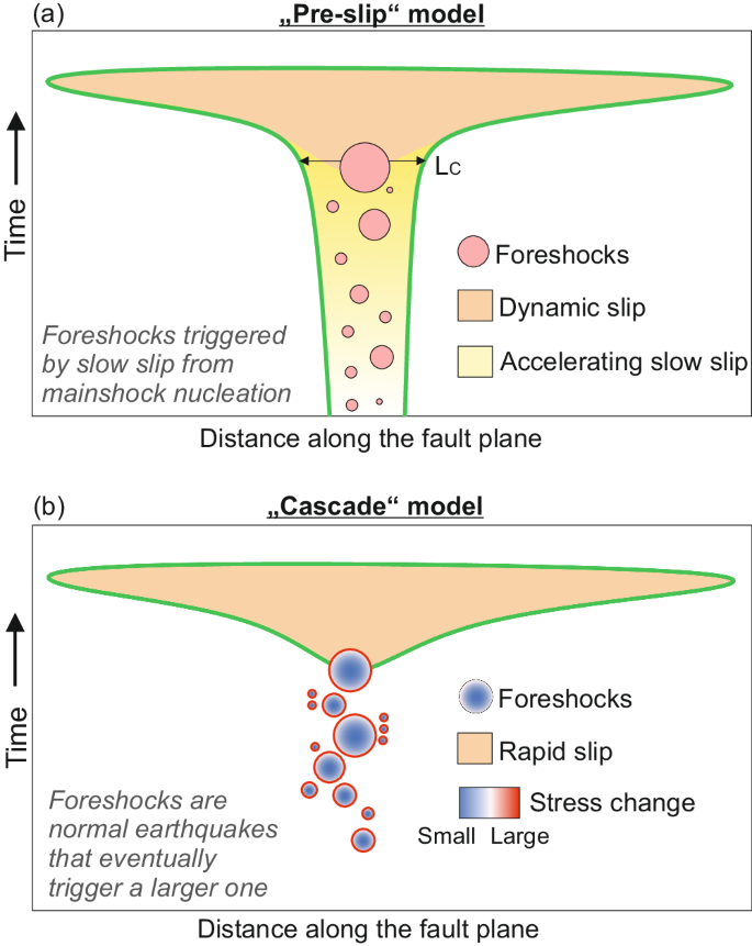
a Pre-slip model, (b) Cascade model. LC: critical nucleation length. The green outline represents the slip front.
-
(2)
The cascade model, in which the stress change associated with the occurrence of each foreshock triggers the next one, and eventually triggers the rupture of a larger earthquake by stress transfer (Fig. 1b). In this model, earthquake nucleation is viewed as a stochastic process in which each foreshock is no different from the mainshock. Therefore, the time and magnitude of the mainshock cannot be inferred before the end of the mainshock rupture27, giving no chance for earthquake predictability37,38.
The physical models described above have often been proposed to explain the seismic and geodetic observations prior to earthquakes in nature29,32,39. However, observations from several sequences also suggest that these two models probably oversimplify the real processes. For example, pre-slip is mostly observed in homogeneous laboratory faults20, which are rarely found in nature. To account for the heterogeneous nature of real faults, new numerical studies15,40,41 and laboratory settings20,42 have been developed. The introduction of stress and strength heterogeneity in the models and experiments began to reveal complicated spatio-temporal patterns of foreshocks and aseismic slip, often resulting from stress feedback processes15, leading to new models describing these more complex deformation patterns.
-
(3)
In the rate-dependent cascade-up model20, the nucleation is characterized by the coexistence of stress transfer (as in the cascade model) and aseismic slip, although the latter is not an intrinsic part of the nucleation process as in the pre-slip model. The heterogeneity in stress or strength strongly controls the nature of the observable processes before the mainshock, and the nucleation of an event is favored by an increase of stress in a rupture-prone fault region.
-
(4)
The progressive localization model43 emerged from recent geophysical observations over longer spatial and temporal scales before large earthquakes, revealing a somewhat larger variability than that captured by the theoretical and laboratory models. The progressive localization model describes a gradual evolution from distributed damage in a rock volume to more localized slip. During this localization process, many clusters of seismicity are expected to be observed within a zone containing multiple faults at different scales. Each cluster may have its own foreshocks, one of which may lead to the initiation of the mainshock rupture. In this model, the presence of an existing fault that is weaker than the surrounding medium is less (or not) relevant43.
-
(5)
With the aim of generalizing the various existing models, an integrated model4 was proposed describing the generation of large earthquakes. The initial phase corresponds to the localization model, with progressive generation of rock damage and ongoing seismicity along the future rupture zone. Foreshocks are driven by the stress transfer from the occurrence of previous seismicity or the presence of aseismic slip. Then, as in the rate-dependent cascade-up model, a foreshock can trigger the large dynamic rupture.

Results: synthesis of observable processes preceding earthquakes
We compiled available studies of 33 earthquake mainshocks spanning a magnitude range MW [3.7–9.0] with the aim of summarizing the inferred physical processes that may drive their occurrence (Fig. 2a). The mainshock inventory includes earthquakes that occurred under various stress, kinematics, fault loading and structural conditions. Where possible, quantitative parameters describing the sequences were extracted from the reviewed articles (Supplementary Table S1). An individual description of each earthquake sequence is provided in Supplementary Note S1. Earthquake preparatory processes are mostly derived from seismic and geodetic observations, which are described separately below.

a Location of the earthquake mainshocks (stars) included in this analysis. Color is encoded with faulting style, with red, green and blue denoting normal, strike-slip and reverse faulting, respectively. Number of seismic events preceding the mainshock versus analyzed time span using catalogs derived with standard (b) and enhanced (c) data analysis techniques, respectively. Colored circles and squares denote sequences where MC or Mmin was available, respectively, where the color is encoded with MC or Mmin. White circles are otherwise utilized. Symbol size is encoded with magnitude. Circles below the panels represent events for which no foreshocks were identified and reported during the analyzed time period. A and B letters after specific earthquakes denote the corresponding catalog if more than one dataset was available (see Table S1 for details and references).
Seismological observables
In most of the studies reviewed, the assessment of mainshock preparation and nucleation was conducted by examining the spatial and temporal evolution of foreshocks. However, rarely were signals quantitatively linked to intrinsic nucleation processes. A possible exception is the M2016 MW 3.7 into Flats earthquake (Event #19 in Supplementary Note 1), where the mainshock was preceded by approximately 20 s of high-frequency radiation and a Very Low Frequency (VLF) earthquake, both located near the mainshock hypocenter44.
When comparing and reviewing different earthquake sequences, an important goal was to explore how the onset of an earthquake preparatory phase was defined. In laboratory experiments, this is typically associated with periods of visible inelastic behavior in the stress-strain curve14,16. Our study revealed that foreshock activity in nature was typically identified as anomalous with respect to the stable background seismicity, but identifying the onset of the stress-strain non-elastic behavior was rarely possible. Additionally, as source parameters (e.g., static stress drop, radiated energy, apparent stress) and the mechanics of foreshocks (e.g., fault orientation, frictional parameters) are a priori no different from mainshocks and aftershocks, there is no unique and unambiguous recipe for recognizing foreshocks before the mainshock occurs. For this reason, many studies defined the foreshock sequences as all the seismicity of smaller magnitude than the mainshock within a predefined time and space window45. The temporal scale typically ranged from minutes to months and the spatial scale from meters to tens of kilometers around the mainshock hypocenter. The spatial and temporal windows selected in some of the early studies were probably designed to capture the short-term slip acceleration predicted by theoretical models12. Additionally, these choices were likely constrained by the absence of continuous geophysical time series covering annual periods until recent years. The application of more objective data analysis43,46, as for example, to the events preceding the 2014 Iquique earthquake47 (see Event #24 in Supplementary Note S1) has helped to achieve a more rigorous estimation of the foreshock sequence.
In the following sections, we first analyze the influence of various monitoring setups and data analysis techniques on the seismic observables. Subsequently, we elucidate the connection between these seismic observables before mainshocks and the underlying physical processes.
Influence of monitoring conditions and data analysis
Ensuring that the monitoring conditions are sufficient to detect foreshocks is essential to correctly infer the physical processes driving the dynamics of the sequences. Our mainshock compilation covers the period from 1986 to 2023. During these years, the number of seismic stations available increased in many of the regions analyzed, resulting in an overall decrease in the magnitude detection threshold (see e.g., Hauksson and Shearer48). In addition, development of advanced data analysis methods over the last decade, such as template matching49,50 and machine learning51 enabled further reductions in the magnitude detection threshold, typically by up to a unit of magnitude. The catalogs for the sequences reviewed were produced employing different data analysis techniques, and utilizing data recorded on seismic networks with different detection thresholds, hence the magnitude of completeness varies considerably (Fig. 2b, c). Differences in data quality between catalogs make it difficult to compare foreshock sequences objectively and may lead to differences in the foreshock rates. Furthermore, a high magnitude of completeness may obscure spatio-temporal foreshock patterns. Nevertheless, most monitoring setups capable of detecting seismicity at least three magnitude units lower than the mainshock detected foreshock activity3.
The analyzed time window preceding the mainshocks from the selected sequences spans from 30 min (for the 2019 MW 6.4 Ridgecrest52, Event #9 in Supplementary Note 1) to nine years (for the 2023 MW 7.8 Kahramanmaraş53,54, Event #3 in Supplementary Table 1). In Fig. 2b, c, we report the number of seismic events preceding the mainshock, as a function of the duration of the analyzed time period and the corresponding magnitude of completeness MC (where available), for seismicity catalogs derived using standard and enhanced techniques, respectively. The median MC of all the compiled catalogs derived by standard techniques is 1.5 (Fig. 2b), but for at least seven sequences (mainly before the year 2000) no MC was reported. In contrast, the median MC of the enhanced seismicity catalogs was reduced to 0.5 (Fig. 2c). The scatter in the observations is larger for seismicity catalogs derived by standard techniques (Fig. 2b) than those derived by enhanced techniques (Fig. 2c), revealing that standard data analysis is greatly affected by the local monitoring conditions. Despite a greater consistency between foreshock rates and analyzed time periods among the enhanced catalogs, there is still significant scatter (Fig. 2c). For example, looking at approximately one day before the mainshock, the number of reported foreshocks included in the enhanced catalogs vary from 50 for the 1999 Hector Mine (Event #7 in Supplementary Note 1) to almost 200 for the 2016 Te Araroa (Event #27 in Supplementary Note 1, Fig. 2b, c).
The variability of the observations presented here reflects to some degree the differences in station coverage and the methodologies employed to build catalogs. Nevertheless, most of the studies also presented quantitative measures of the temporal and spatial evolution of the seismicity (Table S1), associated with the physical processes which are described in Supplementary Note S1 and discussed in the following sections.
Foreshock dynamics from high-resolution catalogs
Upon minimizing differences in the monitoring conditions and data analysis among sequences, various seismic observables such as foreshock rates, moment release or the size of the foreshock area (Figs 2, 3) can be utilized to infer the physical processes in the lead up to an earthquake. In this regard, monitoring the time-space foreshock evolution is a common feature of the studied sequences27,55. Most of the studies analyzed reported that the evolution of foreshocks is connected to the complexity of the physical processes that preceded a mainshock. If foreshocks were a by-product of a single process, a specific time or seismic moment evolution would be expected, such as accelerated seismic release37,56 similar to that observed in laboratory experiments57. However, a simple time evolution (e.g., acceleration) has rarely been observed.

a, b Inter-event time as a function of time to mainshock (gray circles) and cumulative number of events (purple line). Concentrations of gray circles reveal seismicity accelerations. c, d Distance as a function of time to mainshock. Spatial clustering is also observed during periods of accelerated seismicity. Colored boxes mark seismicity clusters discussed in Durand et al.63 and Cabrera et al.64, with their inferred physical mechanism reported in the legend.
The spatio-temporal migration of seismicity can be attributed to various physical mechanisms, such as aseismic slip58, fluid migration59 or stress transfer between earthquakes32. Distinguishing between these mechanisms is aided by assessing the speed of migration60,61. Our analysis of foreshocks revealed a predominant intermittent temporal pattern (refer to Fig. 3a, b) accompanied by distinct spatial migrations (see Fig. 3c, d). These spatiotemporal patterns are interpreted as seismic manifestations arising from a diverse range of physical processes. For instance, foreshock sequences linked to the 2009 L’Aquila event (Event #1 in Supplementary Note 1) and the 2019 Marmara event (Event #31 in Supplementary Note 1) exhibit numerous temporal increments in seismicity (refer to Fig. 3a, b), with migrations partially indicating fluid propagation or aseismic slip, partly afterslip resulting from significant foreshocks, and partly indicative of stress interaction between asperities62,63. Furthermore, for nine of the sequences, foreshock spatiotemporal migrations were reported, with velocities ranging from 2 m/day to 20 km/day (see Supplementary Table 1). Migration velocities below 1 km/day are typically associated with fluid movement, as observed e.g., in the 2016 Pawnee (Event #14 in Supplementary Note S1, see ref. 64) or the 2010 El Mayor-Cucapah (Event #6 in Supplementary Note S1, see ref. 30). On the other hand, faster migration velocities are often linked to slow slip propagation, as exemplified in events like the 2016 Kumamoto (Event #8 in Supplementary Note S1, see ref. 55) or the 2014 Iquique earthquake (Event #24 in Supplementary Note S1, see ref. 65).
In summary, foreshocks exhibit an intermittent and spatio-temporally localized pattern, indicating an interplay of processes rather than directly tracking a single intrinsic mechanism leading to the mainshock. This ensemble of processes occurs over a wide area, as depicted in Fig. 3. A comparable complex behavior is commonly observed both experimentally and in numerical models describing earthquake ruptures on heterogenous faults. In experimental settings, the evolution of Acoustic Emissions (AE) recorded in rock deformation experiments before stick-slip events often showcases clusters of AE events localized in multiple asperities. These clusters tend to coalesce as the fracture approaches, reflecting a behavior similar to that observed in earthquake foreshocks14,16.
Can we learn about the upcoming mainshock size from the foreshocks?
A related topic of crucial importance, with implications for hazard mitigation, is whether the earthquake preparatory and nucleation processes can inform about the upcoming mainshock size. In the pre-slip nucleation model, foreshocks are a by-product of a growing slow slip, and they rupture small brittle asperities within the slow slip area (Fig. 1a). Accordingly, the area covered by the foreshocks could give an indication of the critical nucleation length LC of the mainshock, and hence, of its magnitude. Dodge et al.27 estimated the area activated by the foreshock sequences of six strike-slip mainshocks (assuming a constant stress drop of 3 MPa) and compared the radius of the foreshock area with the mainshock coseismic moment. They found that the extent of the foreshock sequences, representing the size of the nucleation region, roughly scaled with the mainshock seismic moment. Chen and Shearer60 further investigated this scaling for 14 foreshock sequences potentially driven by fluid, and concluded that there was no clear relationship.
We increased the number of observations with our additional sequences. Although this plot may be affected by the magnitude of completeness and the processing choices made by the different studies, it still shows that, the size of the area activated by the foreshocks does indeed tend to increase with mainshock size (Fig. 4), suggesting that aseismic slip may have been involved in mainshock nucleation at the spatial scale delimited by the foreshock sequence. However, several sequences for which an enhanced seismicity catalog is available do not follow such a trend. Among them, the foreshock sequences of strike-slip mainshocks such as the 1999 MW 7.1 Hector Mine (Event #7 in Supplementary Note S1), the 1992 MW 7.3 Landers (Event #5 in Supplementary Note S1) or the 2019 MW 6.4 first Ridgecrest (Event #9 in Supplementary Note S1), activated a smaller area than predicted by the overall trend (Fig. 4). These mainshocks invoke a potential rupture driven by more localized physical processes, such as static stress transfer (e.g., as discussed in Yoon et al.36 for the 1999 MW 7.1 Hector Mine, Event #7 in Supplementary Note S1). Conversely, the foreshock sequences of the 2014 MW 8.1 Iquique (Event #24 in Supplementary Note S1) and 2017 MW 6.9 Valparaiso (Event #29 in Supplementary Note S1) subduction earthquakes activated a broader area than what predicted by this empirical trend (Fig. 4). This suggests that larger scale processes such as subduction slab-pull (see section “Larger-scale processes”) also played an active role in controlling the evolution of the future earthquake region and prepared it for rupture.

Despite the potential trends between foreshock area and mainshock size mentioned above, the self-similarity of earthquakes in nature suggests that some ruptures that start as small earthquakes may grow larger, which is more consistent with the cascade model. Numerical simulations have shown that the final mainshock size is largely controlled by the dynamics of its rupture and propagation66. At the same time, numerical simulations and observations of highly correlated earthquakes in Japan have shown that the existence of hierarchical physics play an important role in controlling the rupture dynamics and hence, the final upcoming mainshock size67,68.
Geodetic observations of slow-slip preceding earthquakes
As with the seismological observations, the vast majority of geodetic studies focusing on the times leading up to large earthquakes showed a significant spatiotemporal complexity, including transient accelerations and afterslip induced by large foreshocks. If a single process with a specific temporal evolution was taking place prior to an earthquake (e.g., acceleration of slip37), we would see its signature in the recorded geodetic deformation. However, none of the studies unambiguously reported an isolated acceleration behavior. Thus, they do not directly trace a process of intrinsic earthquake self-nucleation.
One of the most complex GNSS observations was reported before the 2011 MW 9.0 Tohoku-Oki earthquake (Event #21 in Supplementary Note 1). Prior to the mainshock, a slow transient was recorded in the GNSS instruments, beginning approximately 2 days before the mainshock and following a MW 7.3 foreshock31,69. The recorded aseismic deformation was initially interpreted to be aseismic pre-slip, and thus as evidence for self-nucleation31. Nevertheless, the pre-slip did not manifest within the anticipated future mainshock rupture zone. Additionally, the observed logarithmic temporal decay of the slip aligns with expectations for the afterslip following the MW 7.3 foreshock70. Inversion of the GPS data showed that this recorded aseismic slip preceding the mainshock was the most likely explanation for the occurrence of foreshocks and repeating earthquakes prior to the MW 9.031. Therefore, this recorded aseismic slip (afterslip) probably does not represent pre-slip as an intrinsic nucleation process of the impending MW 9.0, mainly because it did not occur within the future mainshock rupture and decayed with time instead of accelerating. Nevertheless, this slow transient most likely contributed to the stress increase in the future mainshock area and thus to the nucleation of the 2011 MW 9.0 Tohoku-Oki earthquake31,70.
Another sequence highlighting the complex interplay between different slow slip processes prior to earthquakes emerged from the 2017 MW 6.9 Valparaiso earthquake71,72,73 (Event #29 in Supplementary Note 1). The event was preceded by slow deformation recorded by geodetic instruments, which was further evidenced by the occurrence of repeating earthquakes71,74. This aseismic slip started after a MW 6 foreshock and decayed in time, again suggesting the occurrence of afterslip, as before the 2011 Tohoku-Oki earthquake. Caballero et al.72 calculated the slip balance between foreshocks and aseismic slip, and concluded that seismicity and afterslip could account for only half of the observed slip. Moutote et al.73 generated an enhanced catalog of seismicity framing the mainshock. They reported the occurrence of aseismic transients starting one day before the foreshocks and continuing for several days after the mainshock. The authors concluded that the seismicity from this sequence was driven by a slow slip transient that started before the mainshock and continued for several days after it.
Although most geodetic studies showed a complicated time evolution of slip prior to mainshocks, an intriguing new result comes from the joint analysis of GNSS data close to the future nucleation of 93 M > 7 earthquakes worldwide75. By stacking recordings from all these sequences, an accelerating signal starting 2 h before the mainshocks emerged, which could represent a potential precursory signal, intrinsically linked to the nucleation process.
Larger-scale processes
With the collection of decades of geophysical data over entire plate boundary regions, scientists began to look for larger-scale and longer-term signatures of processes leading to large earthquakes. From the analysis of seismic catalogs76, geodetic time series77 and gravity anomalies78 in Japan and Chile at the plate boundary scale, authors reported a long-term (years) slab-pull effect favoring the occurrence of large earthquakes. However, the subtle signals from these studies have been a matter of debate and reported to not be significant by other authors79,80. Other studies highlighted how stress transfer from distant earthquakes (100–1000 km) can affect the fault coupling in some regions of the megathrust and promote the weakening of the interface71,74,81. Such behavior was recently reproduced in laboratory analog experiments recreating subduction zones82.
Earthquake preparation on large spatio-temporal scales has also been investigated for strike-slip faults. Ben-Zion and Zaliapin43 utilized the decades-long Southern California seismicity catalog to show that four of the largest recent earthquakes in California, were preceded in the previous decades by generation of off-fault rock damage around the eventual rupture zones. Seismicity localization around the main fault segments starting 2–3 years before the mainshocks was also reported.
Summary: a conceptual multi-scale model for earthquake preparation and nucleation
From our review analysis, it emerges that the seismic and geodetic observations that precede mainshocks can be affected by the resolution of the monitoring setup and the data processing techniques. Furthermore, the choice of temporal and spatial windows of analysis imprints an upper boundary to the characteristic scales of the physical processes that are possible to resolve. Beyond these differences, we posit that these studies also reveal a genuine diversity of physical processes with different characteristic scales that increase the stress on a fault and ultimately bring it to failure, acting individually or juxtaposed.
Among the reviewed studies, almost no sequence reported observations that can be directly related to the earthquake self-nucleation (with possible exceptions being ref. 44 on the Minto Flats earthquake, see Event 19# in Supplementary Note S1 and Bletery and Nocquet75 in stacks of several sequences as discussed in Section “Geodetic observations of slow-slip preceding earthquakes”). Most of the slow slip observations reported so far in different studies did not represent an intrinsic part of the nucleation. This suggests that, if self-nucleation processes as those resolved in laboratory experiments occur at larger scale in nature, their detection is very difficult83. This may be because their associated signals are likely to be too small in amplitude or too short in time, and are often convolved with other processes, which prevents them from being systematically identified by our current instrumentation and data analysis techniques.
Foreshocks are the most common observation preceding earthquakes26,27, but most studies support the notion that foreshocks are a by-product of processes that alter the state of stress in a given fault and reflect its heterogeneities. Only rarely we observe clear foreshock accelerations as predicted by numerical modeling or in some laboratory experiments10,14,15,20,84,85,86,87,88. When it does occur, acceleration is typically observed on a regional scale rather than being part of a localized process53. More often, foreshocks occur in spatiotemporal clusters likely to represent creep surges15, fluid pressure fluctuations89, or temporal clustering associated with static and dynamic triggering32,36. In the laboratory, analogous complexities in the observations and feedbacks between different processes are more evident at fractured fault interfaces with many asperities of variable roughness90.
In most studies of the sequences analyzed, a shear stress increment in the future mainshock rupture area was inferred, either by Coulomb stress transfer analysis or Brune stress drop calculation or through monitoring of indirect stress proxies, e.g., by resolving a temporal decrease in the Gutenberg-Richter b-value. This stress increase can be due to a large variety of physical processes (some of the most important listed in Fig. 5), as for example stress transfer from previous seismicity32, the occurrence and propagation of slow slip transients91, the migration of fluids along a fault patch resulting in a pore fluid pressure increase92,93 or any combination of these and additional mechanisms. Each of these mechanisms can operate at a different spatial scale, and they can also temporally vary. The spatial and temporal scales at which each of these processes may operate are influenced by the heterogeneities of the medium and connected to the fault geology, rheology, geometry, and segmentation. Larger heterogeneities in the medium are translated into corresponding heterogeneities in the state of stress at different scales.

Chart summarizing some of the identified physical processes (in black Roman) and seismological and geodetic observables (in blue italics) that occur prior to mainshocks at various spatial and temporal scales.
Taken together, the observations from our review emphasize the distinctiveness of each mainshock, marked by its unique stress history across various scales, and leading to slightly different preparation phases for each event. Considered alongside variations in the resolution and magnitude of completeness in different studies, these disparities offer an explanation to the lack of scaling observed in several parameters extracted from the reviewed studies (Supplementary Table S1). Building on these findings, we propose a conceptual model in which the preparation and nucleation of earthquakes are shaped by a diverse array of physical processes, sometimes acting juxtaposed. These processes operate on different temporal and spatial scales, collectively contributing to stress build-up and fault slip (refer to Figs 5 and 6).

Conceptual sketch illustrating some of the physical mechanisms at different spatio-temporal scales that may be involved in the preparation and nucleation of an earthquake. Temporal scales represent approximately (a) from hours to days, (b) from days to months and (c) from months to years.
Experimental work, numerical modeling and field observations indicate that the earthquake preparatory process includes damage localization, coalesce of fault segments leading to the failure of larger asperities and enhanced interaction of seismic and aseismic deformation4,15,25,43,94,95. Each of these processes leads to variations in the stress field operating at different spatial scales, and reflecting different heterogeneities and temporal evolution over the fault zone.
A multi-scale model for earthquake preparation is also supported by experimental data. Acoustic emissions recorded during rock deformation experiments on rough faults documented that the evolution of the employed seismo-mechanical parameters (e.g., b-value, clustering properties, event proximity, fault plane and stress variability, etc) displayed different trends depending on the different spatio-temporal scales considered. This supports the notion of a diversity of physical processes acting juxtaposed at different scales during the earthquake preparatory process95. As stress heterogeneities over various lengths are observed to increase with increased roughness and fault heterogeneity, our model might be more representative for seismic sequences occurring on juvenile or segmented fault structures.
The evolution of stress at the future mainshock hypocenter can be additionally influenced by other large-scale external processes such as seasonal or multiannual stress variations96 and tidal stress evolution97,98,99 which can either promote or inhibit the stress build-up on the fault, and hence, trigger or delay the nucleation of earthquakes. Finally, anthropogenic activities such as subsurface mining, fluid injection and extraction, or reservoir impoundment can also perturb the stress field over a wide spatio-temporal scale from the source region. These additional sources of stress perturbation add to those discussed in our work, and further complicate the time-dependent stress state of a fault (Figs 5, 6).
Research perspectives
Decades of research into the nucleation and preparation of tectonic earthquakes suggest that a multitude of physical processes operating on different temporal and spatial scales can influence the stress state of a fault, ultimately leading to its failure (Fig. 6). The interplay of different physical processes, combined with heterogeneous local and regional monitoring conditions, control which seismic and geodetic observables precede mainshocks. Recent detailed studies of observable slip processes before earthquakes represent a significant advancement in documenting the complexity inherent to the development of each earthquake sequence. These studies can now serve as examples for a more systematic evaluation of future mainshock initiation. To gain new insights on the preparation and nucleation of earthquakes, a collaborative effort is essential, involving laboratory experimental studies, the development of theoretical models and the monitoring of observables in natural settings. Here we summarize some of the relevant aspects of this collective endeavor.
-
(i)
Densification of near-fault monitoring. Densification of near-fault seismic and geodetic monitoring is the most pressing need to gain insights into the fault activity prior to mainshock ruptures100. Improving the resolution can enable the detection and characterization of smaller foreshock activity, or resolve subtle geodetic signatures of aseismic processes or fluid movements, thus shedding more light on the underlying mechanisms3. An optimal seismic monitoring network can greatly contribute to the elucidation of fault behavior prior to a large earthquake, such as in the 2023 MW 7.8 Kahramanmaraş earthquake53,54. As we are witnessing that large earthquakes nucleate not only along main fault strands but also on secondary branches, these efforts should not be limited to main fault zones.
-
(ii)
Next-generation observations of fault processes over different frequency bands. Along with the need for instrumental development, there is a need to incorporate cutting-edge data. So far, we have seen how enhanced seismicity catalogs with a lower magnitude of completeness effectively illuminate what happens before the mainshock rupture (i.e., Fig. 2). A necessary step is to continue to generate enhanced observations for past and future earthquakes spanning different magnitudes, faulting styles and background stress conditions, with the aim of extracting similarities and differences between sequences. To this end, data analysis techniques employing artificial intelligence have a tremendous potential to boost fault signal observations51,101,102, which, in turn, may lead to clearer observations of earthquake preparatory processes.
-
(iii)
Automated multi-parametric and multi-scale workflows. With high-resolution data and cutting-edge methods there will be the need to develop and test automated workflows based on time series of parameters103 or data features104,105,106 covering a wide range of spatiotemporal scales. Such workflows could shed light on which physical processes are most important in the preparation and nucleation of each mainshock, and at which scales these processes are most resolvable. They could also help to distinguish between the different juxtaposed physical processes operating at different spatiotemporal scales.
-
(iv)
Identifying the onset of the preparatory phase. Experimentally, the onset of the preparatory phase is typically considered to be the time when the stress-strain curve leaves the elastic regime and the specimen deforms non-linearly. A promising research target is to determine whether the observables that we are able to monitor on faults in nature (e.g., clustering of seismicity, geodetic signals, increased energy release) are anomalous with respect to the stable conditions, and thus, represent part of the preparatory stage. For example, to be able to distinguish whether a burst of earthquakes is unlikely to continue (forming a so-called swarm) or, on the contrary, it could destabilize a fault towards a large rupture. To this end, underground laboratory experiments under controlled conditions have the potential to bridge the gap between the controlled conditions of laboratory experiments and the greater heterogeneity and complexity of faults in nature. For real faults, catching the evolution of susceptibility of earthquake triggering to periodic stresses (e.g., tides) might help to better identify those times in which a fault enters a critical state and is getting closer to the rupture, as recently suggested by laboratory107,108 and field works98,99.
-
(v)
Revised physical frameworks describing earthquake nucleation. Some well-documented processes preceding failure in experiments and nature suggest an interaction between localized seismicity clusters around the future mainshock, and a complex interplay between seismic and aseismic deformation. This behavior is not yet well reflected in commonly used physical frameworks describing earthquake nucleation such as the rate-and-state or slip weakening models. Therefore, there is also a need to revise these frameworks according to the new observations, perhaps allowing for a greater level of complexity or larger spatial and temporal scales.
References
Wyss, M. “Cannot earthquakes be predicted?”. Science 278, 487–490 (1997).
Bouchon, M., Durand, V., Marsan, D., Karabulut, H. & Schmittbuhl, J. The long precursory phase of most large interplate earthquakes. Nat. Geosci. 6, 299–302 (2013).
Mignan, A. The debate on the prognostic value of earthquake foreshocks: a meta-analysis. Sci. Rep. 4, 4099 (2014).
Kato, A., & Ben-Zion, Y. The generation of large earthquakes. Nat. Rev. Earth Environ. 1–14. https://doi.org/10.1038/s43017-020-00108-w (2020).
Gomberg, J. Unsettled earthquake nucleation. Nat. Geosci. 11, 463–464 (2018).
Gualandi, A., Avouac, J.-P., Michel, S. & Faranda, D. The predictable chaos of slow earthquakes. Sci. Adv. 6, eaaz5548 (2020).
Okubo, P. G. & Dieterich, J. H. Effects of physical fault properties on frictional instabilities produced on simulated faults. J. Geophys. Res. Solid Earth 89, 5817–5827 (1984).
Scholz, C. H. Earthquakes and friction laws. Nature 391, 37–42 (1998).
Rice, J. R. Constitutive relations for fault slip and earthquake instabilities. Pure Appl. Geophys. 121, 443–475 (1983).
Dieterich, J. H. Earthquake nucleation on faults with rate-and state-dependent strength. Tectonophys. 211, 115–134 (1992).
Rice, J. R. & Ruina, A. L. Stability of steady frictional slipping. J. Appl. Mech. 50, 343–349 (1983).
Ohnaka, M. Earthquake source nucleation: a physical model for short-term precursors. Tectonophysics 211, 149–178 (1992).
Ohnaka, L.-f., & Lin‐feng, S. Scaling of the shear rupture process from nucleation to dynamic propagation: Implications of geometric irregularity of the rupturing surfaces. J. Geophys. Res. 104, 817–844 (1999).
Dresen, G., Kwiatek, G., Goebel, T. & Ben-Zion, Y. Seismic and aseismic preparatory processes before large stick–slip failure. Pure Appl. Geophys. 177, 5741–5760 (2020).
Cattania, C. & Segall, P. Precursory slow slip and foreshocks on rough faults. J. Geophys. Res. Solid Earth 126, e2020JB020430 (2021).
Marty, S. et al. Nucleation of laboratory earthquakes: quantitative analysis and scalings. J. Geophys. Res. Solid Earth 128, e2022JB026294 (2023).
Guérin‐Marthe, S., Nielsen, S., Bird, R., Giani, S. & Toro, G. D. Earthquake nucleation size: evidence of loading rate dependence in laboratory faults. J. Geophys. Res. Solid Earth 124, 689–708 (2019).
Selvadurai, P. A., Glaser, S. D., & Parker, J. M. On factors controlling precursor slip fronts in the laboratory and their relation to slow slip events in nature. Geophys. Res. Lett. 2017GL072538. https://doi.org/10.1002/2017GL072538 (2017).
Latour, S., Schubnel, A., Nielsen, S., Madariaga, R. & Vinciguerra, S. Characterization of nucleation during laboratory earthquakes. Geophys. Res. Lett. 40, 5064–5069 (2013).
McLaskey, G. C. Earthquake initiation from laboratory observations and implications for foreshocks. J. Geophys. Res. Solid Earth 124, 12882–12904 (2019).
Passelègue, F. X. et al. Influence of fault strength on precursory processes during laboratory earthquakes. In Fault Zone Dynamic Processes 229–242 (American Geophysical Union, 2017).
Scuderi, M. M. & Collettini, C. The role of fluid pressure in induced vs. triggered seismicity: insights from rock deformation experiments on carbonates. Sci. Rep. 6, 24852 (2016).
Scuderi, M. M. & Collettini, C. Fluid injection and the mechanics of frictional stability of shale-bearing faults. J. Geophys. Res. Solid Earth 123, 8364–8384 (2018).
Cebry, S. B. L. & McLaskey, G. C. Seismic swarms produced by rapid fluid injection into a low permeability laboratory fault. Earth Planet. Sci. Lett. 557, 116726 (2021).
Renard, F. et al. Microscale characterization of rupture nucleation unravels precursors to faulting in rocks. Earth Planet. Sci. Lett. 476, 69–78 (2017).
Abercrombie, R. E. & Mori, J. Occurrence patterns of foreshocks to large earthquakes in the western United States. Nature 381, 303–307 (1996).
Dodge, D. A., Beroza, G. C. & Ellsworth, W. L. Detailed observations of California foreshock sequences: implications for the earthquake initiation process. J. Geophys. Res. Solid Earth 101, 22371–22392 (1996).
McGuire, J. J. Immediate foreshock sequences of oceanic transform earthquakes on the East Pacific Rise. Bullet. Seismol. Soc. Am. 93, 948–952 (2003).
Bouchon, M. et al. Extended nucleation of the 1999 Mw 7.6 Izmit earthquake. Science 331, 877–880 (2011).
Yao, D., Huang, Y., Peng, Z. & Castro, R. R. Detailed investigation of the foreshock sequence of the 2010 Mw7.2 El Mayor-Cucapah Earthquake. J. Geophys. Res. Solid Earth 125, e2019JB019076 (2020).
Kato, A. et al. Propagation of slow slip leading up to the 2011 Mw 9.0 Tohoku-Oki earthquake. Science 335, 705–708 (2012).
Ellsworth, W. L. & Bulut, F. Nucleation of the 1999 Izmit earthquake by a triggered cascade of foreshocks. Nat. Geosci. 11, 531 (2018).
Beroza, G. C. & Ellsworth, W. L. Properties of the seismic nucleation phase. Tectonophysics 261, 209–227 (1996).
McGuire, J. J., Boettcher, M. S. & Jordan, T. H. Foreshock sequences and short-term earthquake predictability on East Pacific Rise transform faults. Nature 434, 457–461 (2005).
Ellsworth, W. L. & Beroza, G. C. Seismic evidence for an earthquake nucleation phase. Science 268, 851 (1995).
Yoon, C. E., Yoshimitsu, N., Ellsworth, W. L. & Beroza, G. C. Foreshocks and mainshock nucleation of the 1999 Mw 7.1 hector mine, California, earthquake. J. Geophys. Res. Solid Earth 124, 1569–1582 (2019).
Mignan, A. Retrospective on the accelerating seismic release (ASR) hypothesis: controversy and new horizons. Tectonophysics 505, 1–16 (2011).
Münchmeyer, J., Leser, U. & Tilmann, F. A probabilistic view on rupture predictability: all earthquakes evolve similarly. Geophys. Res. Lett. 49, e2022GL098344 (2022).
Kato, A., Fukuda, J., Kumazawa, T. & Nakagawa, S. Accelerated nucleation of the 2014 Iquique, Chile Mw 8.2 Earthquake. Sci. Rep. 6, 24792 (2016).
Tal, Y., Hager, B. H. & Ampuero, J. P. The effects of fault roughness on the earthquake nucleation process. J. Geophys. Res. Solid Earth 123, 437–456 (2018).
Noda, H., Nakatani, M. & Hori, T. Large nucleation before large earthquakes is sometimes skipped due to cascade-up—Implications from a rate and state simulation of faults with hierarchical asperities. J. Geophys. Res. Solid Earth 118, 2924–2952 (2013).
Yamashita, F. et al. Two end-member earthquake preparations illuminated by foreshock activity on a meter-scale laboratory fault. Nat. Commun. 12, 4302 (2021).
Ben-Zion, Y. & Zaliapin, I. Localization and coalescence of seismicity before large earthquakes. Geophysical Journal International 223, 561–583 (2020).
Tape, C. et al. Earthquake nucleation and fault slip complexity in the lower crust of central Alaska. Nat. Geosci. 11, 536–541 (2018).
Shearer, P. M. & Lin, G. Evidence for Mogi doughnut behavior in seismicity preceding small earthquakes in southern California. J. Geophys. Res. 114, B01318 (2009).
Baiesi, M. & Paczuski, M. Scale-free networks of earthquakes and aftershocks. Phys. Rev. E 69, 066106 (2004).
Aden‐Antóniow, F. et al. Statistical analysis of the preparatory phase of the M w 8.1 Iquique Earthquake, Chile. J. Geophys. Res. Solid Earth 125, e2019JB019337 (2020).
Hauksson, E. & Shearer, P. Southern California hypocenter relocation with waveform cross-correlation, part 1: results using the double-difference method. Bullet. Seismol. Soc. Am. 95, 896–903 (2005).
Gibbons, S. J. & Ringdal, F. The detection of low magnitude seismic events using array-based waveform correlation. Geophys. J. Int. 165, 149–166 (2006).
Shelly, D. R., Beroza, G. C., Ide, S. & Nakamula, S. Low-frequency earthquakes in Shikoku, Japan, and their relationship to episodic tremor and slip. Nature 442, 188–191 (2006).
Beroza, G. C., Segou, M. & Mostafa Mousavi, S. Machine learning and earthquake forecasting—next steps. Nat. Commun. 12, 4761 (2021).
Huang, Hui et al. Spatio-temporal foreshock evolution of the 2019 M 6.4 and M 7.1 Ridgecrest, California earthquakes. Earth Planet. Sci. Lett. 551, 116582 (2020).
Kwiatek, G. et al. Months-long preparation of the 2023 MW 7.8 Kahramanmaraş earthquake, Türkiye. Nat. Commun. https://doi.org/10.21203/rs.3.rs-2657873/v1 (2023).
Picozzi, M., Iaccarino, A. G. & Spallarossa, D. The preparatory process of the 2023 Mw 7.8 Türkiye earthquake. Sci. Rep. 13, 17853 (2023).
Kato, A., Fukuda, J., Nakagawa, S. & Obara, K. Foreshock migration preceding the 2016 Mw 7.0 Kumamoto earthquake, Japan. Geophys. Res. Lett. 43, 8945–8953 (2016a).
Hough, S. Predicting the Unpredictable: The Tumultuous Science of Earthquake Prediction 272 (Princeton University Press, 2010).
Schubnel, A., Thompson, B. D., Fortin, J., Guéguen, Y. & Young, R. P. Fluid-induced rupture experiment on Fontainebleau sandstone: premonitory activity, rupture propagation, and aftershocks. Geophys. Res. Lett. 34, L19307 (2007).
Perfettini, H., & Avouac, J.-P. Postseismic relaxation driven by brittle creep: A possible mechanism to reconcile geodetic measurements and the decay rate of aftershocks, application to the Chi-Chi earthquake, Taiwan. J. Geophys. Res. Solid Earth 109. https://doi.org/10.1029/2003JB002488 (2004).
Shapiro, S. A., Patzig, R., Rothert, E. & Rindschwentner, J. Triggering of seismicity by pore-pressure perturbations: permeability-related signatures of the phenomenon. Pure Appl. Geophys. 160, 1051–1066 (2003).
Chen, X. & Shearer, P. M. Analysis of foreshock sequences in California and implications for earthquake Triggering. Pure Appl. Geophys. 173, 133–152 (2016).
Fischer, T. & Hainzl, S. The growth of earthquake clusters. Front. Earth Sci. 9, 79 (2021).
Durand, V. et al. A two‐scale preparation phase preceded an Mw 5.8 earthquake in the sea of Marmara Offshore Istanbul, Turkey. Seismol. Res. Lett. 91, 3139–3147 (2020).
Cabrera, L., Poli, P. & Frank, W. B. Tracking the spatio-temporal evolution of foreshocks preceding the Mw 6.1 2009 L’Aquila earthquake. J. Geophys. Res. Solid Earth 127, e2021JB023888 (2022).
Chen, X. et al. The Pawnee earthquake as a result of the interplay among injection, faults and foreshocks. Sci. Rep. 7, 4945 (2017).
Kato, A. & Nakagawa, S. Multiple slow‐slip events during a foreshock sequence of the 2014 Iquique, Chile Mw 8.1 earthquake. Geophys. Res. Lett. 41, 5420–5427 (2014).
Okubo, K. et al. Dynamics, radiation, and overall energy budget of earthquake rupture with coseismic off-fault damage. J. Geophys. Res. Solid Earth 124, 11771–11801 (2019).
Ide, S., & Aochi, H. Earthquakes as multiscale dynamic ruptures with heterogeneous fracture surface energy. J. Geophys. Res. Solid Earth 110 https://doi.org/10.1029/2004JB003591 (2005).
Okuda, T. & Ide, S. Hierarchical rupture growth evidenced by the initial seismic waveforms. Nat. Commun. 9, 3714 (2018).
Hino, R. et al. Was the 2011 Tohoku-Oki earthquake preceded by aseismic preslip? Examination of seafloor vertical deformation data near the epicenter. Marine Geophys. Res. 35, 181–190 (2014).
Otha, Y. et al. Geodetic constraints on afterslip characteristics following the March 9, 2011, Sanriku-Oki earthquake, Japan. Geophys. Res. Lett. 39 https://doi.org/10.1029/2012GL052430 (2012).
Ruiz, S. et al. The Seismic Sequence of the 16 September 2015 Mw 8.3 Illapel, Chile, Earthquake. Seismol. Res. Lett. 87, 789–799 (2016).
Caballero, E. et al. Seismic and Aseismic fault slip during the initiation phase of the 2017 MW = 6.9 Valparaíso earthquake. Geophys. Res. Lett. 48, e2020GL091916 (2021).
Moutote, L., Itoh, Y., Lengliné, O., Duputel, Z. & Socquet, A. Evidence of a transient aseismic slip driving the 2017 Valparaiso earthquake sequence, from Foreshocks to Aftershocks. J. Geophys. Res. Solid Earth 128, e2023JB026603 (2023).
Ruiz, S. et al. Nucleation phase and dynamic inversion of the Mw 6.9 Valparaíso 2017 earthquake in Central Chile. Geophys. Res. Lett. 44, 10,290–10,297 (2017).
Bletery, Q. & Nocquet, J.-M. The precursory phase of large earthquakes. Science 381, 297–301 (2023).
Bouchon, M. et al. Potential slab deformation and plunge prior to the Tohoku, Iquique and Maule earthquakes. Nat. Geosci. 9, 380–383 (2016).
Bedford, J. R. et al. Months-long thousand-kilometre-scale wobbling before great subduction earthquakes. Nature 580, 628–635 (2020).
Panet, I., Bonvalot, S., Narteau, C., Remy, D. & Lemoine, J.-M. Migrating pattern of deformation prior to the Tohoku-Oki earthquake revealed by GRACE data. Nat. Geosci. 11, 367–373 (2018).
Delbridge, B. G. et al. Temporal variation of intermediate-depth earthquakes around the time of the M9.0 Tohoku-oki earthquake. Geophys. Res. Lett. 44, 3580–3590 (2017).
Wang, L. & Burgmann, R. Statistical significance of precursory gravity changes before the 2011 Mw 9.0 Tohoku-Oki earthquake. Geophys. Res. Lett. 46, 7323–7332 (2019).
Melnick, D. et al. The super-interseismic phase of the megathrust earthquake cycle in Chile. Geophys. Res. Lett. 44, 784–791 (2017).
Corbi, F., Bedford, J., Poli, P., Funiciello, F. & Deng, Z. Probing the seismic cycle timing with coseismic twisting of subduction margins. Nat. Commun. 13, 1911 (2022).
Roeloffs, E. A. Evidence for aseismic deformation rate changes prior to earthquakes. Ann. Rev. Earth Planet. Sci. 34, 591–627 (2006).
Rubin, A. M. & Ampuero, J.-P. Earthquake nucleation on (aging) rate and state faults. J. Geophys. Res. Solid Earth 110, B11312 (2005).
Ampuero, J. & Rubin, A. Earthquake nucleation on rate and state faults—aging and slip laws. J. Geophys. Res. 113, B0105E (2008).
Dieterich, J. H. & Kilgore, B. Implications of fault constitutive properties for earthquake prediction. Proc. Natl. Acad. Sci. USA 93, 3787–3794 (1996).
McLaskey, G. C. & Kilgore, B. D. Foreshocks during the nucleation of stick-slip instability. J. Geophys. Res. Solid Earth 118, 2982–2997 (2013).
McLaskey, G. C. & Lockner, D. A. Shear failure of a granite pin traversing a sawcut fault. Int. J. Rock Mech. Mining Sci. 110, 97–110 (2018).
Lucente, F. P. et al. Temporal variation of seismic velocity and anisotropy before the 2009 Mw 6.3 L’Aquila earthquake, Italy. Geology 38, 1015–1018 (2010).
Gounon, A., Latour, S., Letort, J. & El Arem, S. Rupture nucleation on a periodically heterogeneous interface. Geophys. Res. Lett. 49, e2021GL096816 (2022).
Radiguet, M. et al. Triggering of the 2014 Mw7.3 Papanoa earthquake by a slow slip event in Guerrero, Mexico. Nat. Geosci. 9, 829–833 (2016).
Chiarabba, C., De Gori, P., Cattaneo, M., Spallarossa, D. & Segou, M. Faults geometry and the role of fluids in the 2016–2017 Central Italy Seismic Sequence. Geophys. Res. Lett. 45, 6963–6971 (2018).
Moreno, M. et al. Locking of the Chile subduction zone controlled by fluid pressure before the 2010 earthquake. Nat. Geosci. 7, 292–296 (2014).
McBeck, J., Ben-Zion, Y. & Renard, F. Volumetric and shear strain localization throughout triaxial compression experiments on rocks. Tectonophysics 822, 229181, https://doi.org/10.1016/j.tecto.2021.229181 (2022).
Kwiatek, G. et al. Intermittent criticality multi-scale processes leading to large slip events on rough laboratory faults. J. Geophys. Res.: Solid Earth. 129, e2023JB028411, https://doi.org/10.1029/2023JB028411 (2024).
Johnson, C. W., Fu, Y. & Bürgmann, R. Seasonal water storage, stress modulation, and California seismicity. Science 356, 1161–1164 (2017).
Tanaka, S. Tidal triggering of earthquakes precursory to the recent Sumatra megathrust earthquakes of 26 December 2004 (Mw 9.0), 28 March 2005 (Mw 8.6), and 12 September 2007 (Mw 8.5). Geophys. Res. Lett. 37, https://doi.org/10.1029/2009GL041581 (2010).
Martínez-Garzón, P., Beroza, G. C., Bocchini, G. M. & Bohnhoff, M. Sea level changes affect seismicity rates in a hydrothermal system near Istanbul. Geophys. Res. Lett. 50, e2022GL101258 (2023).
Beaucé, E., Poli, P., Waldhauser, F., Holtzman, B. & Scholz, C. Enhanced tidal sensitivity of seismicity before the 2019 magnitude 7.1 Ridgecrest, California earthquake. Geophys. Res. Lett. 50, e2023GL104375 (2023).
Ben‐Zion, Y., Beroza, G. C., Bohnhoff, M., Gabriel, A. & Mai, P. M. A grand challenge international infrastructure for earthquake science. Seismol. Res. Lett. 93, 2967–2968 (2022).
Bergen, K. J., Johnson, P. A., de Hoop, M. V. & Beroza, G. C. Machine learning for data-driven discovery in solid Earth geoscience. Science 363, eaau0323 (2019).
Mousavi, S. M., Ellsworth, W. L., Zhu, W., Chuang, L. Y. & Beroza, G. C. Earthquake transformer—an attentive deep-learning model for simultaneous earthquake detection and phase picking. Nat. Commun. 11, 3952 (2020).
Rouet-Leduc, B. et al. Machine learning predicts laboratory earthquakes. Geophys. Res. Lett. 44, 9276–9282 (2017).
Hulbert, C. et al. Similarity of fast and slow earthquakes illuminated by machine learning. Nat. Geosci. 12, 69–74 (2019).
Seydoux, L. et al. Clustering earthquake signals and background noises in continuous seismic data with unsupervised deep learning. Nat. Commun. 11, 3972 (2020).
Shi, P., Seydoux, L. & Poli, P. Unsupervised learning of seismic wavefield features: clustering continuous array seismic data during the 2009 L’Aquila earthquake. J. Geophys. Res. Solid Earth 126, e2020JB020506 (2021).
Chanard, K. et al. Sensitivity of acoustic emission triggering to small pore pressure cycling perturbations during brittle creep. Geophys. Res. Lett. 46, 7414–7423 (2019).
Colledge, M. et al. Susceptibility of microseismic triggering to small sinusoidal stress perturbations at the laboratory scale. J. Geophys. Res. Solid Earth 128, e2022JB025583 (2023).
Saffer, D. M., Frye, K. M., Marone, C. & Mair, K. Laboratory results indicating complex and potentially unstable frictional behavior of smectite clay. Geophys. Res. Lett. 28, 2297–2300 (2001).
Kurzawski, R. M., Stipp, M., Niemeijer, A. R., Spiers, C. J. & Behrmann, J. H. Earthquake nucleation in weak subducted carbonates. Nat. Geosci. 9, 717–722 (2016).
Marone, C., Raleigh, C. B. & Scholz, C. H. Frictional behavior and constitutive modeling of simulated fault gouge. J. Geophys. Res. Solid Earth 95, 7007–7025 (1990).
Kaduri, M., Gratier, J.-P., Renard, F., Çakir, Z., & Lasserre, C. The implications of fault zone transformation on aseismic creep: example of the North Anatolian Fault, Turkey. J. Geophys. Res. Solid Earth 2016JB013803. https://doi.org/10.1002/2016JB013803 (2016).
Bürgmann, R. The geophysics, geology and mechanics of slow fault slip. Earth Planet. Sci. Lett. 495, 112–134 (2018).
Harris, R. A. Large earthquakes and creeping faults. Rev. Geophys. 2016RG000539. https://doi.org/10.1002/2016RG000539 (2017).
McGuire, J. J. et al. Variations in earthquake rupture properties along the Gofar transform fault, East Pacific Rise. Nat. Geosci. 5, 336–341 (2012).
Candela, T., Renard, F., Schmittbuhl, J., Bouchon, M. & Brodsky, E. E. Fault slip distribution and fault roughness. Geophys. J. Int. 187, 959–968 (2011).
Goebel, T. H. W., Schorlemmer, D., Becker, T. W., Dresen, G. & Sammis, C. G. Acoustic emissions document stress changes over many seismic cycles in stick-slip experiments. Geophys. Res. Lett. 40, 2049–2054 (2013).
Harbord, C. W. A., Nielsen, S. B., De Paola, N. & Holdsworth, R. E. Earthquake nucleation on rough faults. Geology 45, 931–934 (2017).
Guérin-Marthe, S. et al. Preparatory slip in laboratory faults: effects of roughness and load point velocity. J. Geophys. Res. Solid Earth 128, e2022JB025511 (2023).
Cochran, E. S., Page, M. T., van der Elst, N. J., Ross, Z. E. & Trugman, D. T. Fault roughness at seismogenic depths and links to earthquake behavior. Seismic Record 3, 37–47 (2023).
Mai, P. M., & Beroza, G. C. A spatial random field model to characterize complexity in earthquake slip. J. Geophys. Res. Solid Earth 107, ESE 10-1-ESE 10-21 https://doi.org/10.1029/2001JB000588 (2002).
Thakur, P. & Huang, Y. Influence of fault zone maturity on fully dynamic earthquake cycles. Geophys. Res. Lett. 48, e2021GL094679 (2021).
Romanet, P., Bhat, H. S., Jolivet, R. & Madariaga, R. Fast and slow slip events emerge due to fault geometrical complexity. Geophys. Res. Lett. 45, 4809–4819 (2018).
Dodge, D. A., Beroza, G. C. & Ellsworth, W. L. Foreshock sequence of the 1992 Landers, California, earthquake and its implications for earthquake nucleation. J. Geophys. Res. Solid Earth 100, 9865–9880 (1995).
Campillo, M. & Ionescu, I. R. Initiation of antiplane shear instability under slip dependent friction. J. Geophys. Res. Solid Earth 102, 20363–20371 (1997).
Leeman, J. R., Saffer, D. M., Scuderi, M. M. & Marone, C. Laboratory observations of slow earthquakes and the spectrum of tectonic fault slip modes. Nat. Commun. 7, 11104 (2016).
Chen, K. H., Bürgmann, R., Nadeau, R. M., Chen, T. & Lapusta, N. Postseismic variations in seismic moment and recurrence interval of repeating earthquakes. Earth Planet. Sci. Lett. 299, 118–125 (2010).
Becker, D., Martínez-Garzón, P., Wollin, C., Kılıç, T. & Bohnhoff, M. Variation of fault creep along the overdue Istanbul-Marmara Seismic Gap in NW Türkiye. Geophys. Res. Lett. 50, e2022GL101471 (2023).
Wang, Z., Fukao, Y., Kodaira, S., & Huang, R. (2008). Role of fluids in the initiation of the 2008 Iwate earthquake (M7.2) in northeast Japan. Geophys. Res. Lett. 35 https://doi.org/10.1029/2008GL035869 (2008).
Guglielmi, Y., Cappa, F., Avouac, J.-P., Henry, P. & Elsworth, D. Seismicity triggered by fluid injection–induced aseismic slip. Science 348, 1224–1226 (2015).
Viesca, R. C. & Rice, J. R. Nucleation of slip-weakening rupture instability in landslides by localized increase of pore pressure. J. Geophys. Res. Solid Earth 117, B03104 (2012).
Marone, C. Laboratory-derived friction laws and their application to seismic faulting. Ann. Rev. Earth Planet. Sci. 26, 643–696 (1998).
Passelègue, F. X. et al. Initial effective stress controls the nature of earthquakes. Nat. Commun. 11, 5132 (2020).
Acknowledgements
P.M.G. acknowledges funding from the Helmholtz Association in the frame of the Young Investigators Group VH-NG-1232 (SAIDAN) and ERC Starting Grant 101076119 (QUAKEHUNTER). P.P. acknowledges the funding from the European Research Council (ERC) under the European Union Horizon 2020 Research and Innovation Program (grant agreements 802777- MONIFAULTS). We thank Georg Dresen, Grzegorz Kwiatek, Yehuda Ben-Zion, Virginie Durand, Frederik Tilmann and Marco Bohnhoff for constructive comments and feedback on this manuscript. Ursula Heidbach provided valuable help with Fig. 6. We also thank Aitaro Kato and Emily Warren-Smith for providing seismicity catalogs for some of the sequences here analyzed. We thank the Editor Luca dal Zilio, Roland Bürgmann and two anonymous reviewers whose valuable feedback contributed to improve the paper.
Funding
Open Access funding enabled and organized by Projekt DEAL.
Author information
Authors and Affiliations
Contributions
Both P.M.G. and P.P. envisioned the review, performed the research literature review, discussed the collective patterns and wrote the article together.
Corresponding author
Ethics declarations
Competing interests
The authors declare no competing interests.
Peer review
Peer review information
Communications Earth & Environment thanks Roland Burgmann and the other, anonymous, reviewer(s) for their contribution to the peer review of this work. Primary Handling Editors: Luca Dal Zilio and Joe Aslin. A peer review file is available.
Additional information
Publisher’s note Springer Nature remains neutral with regard to jurisdictional claims in published maps and institutional affiliations.
Supplementary information
Rights and permissions
Open Access This article is licensed under a Creative Commons Attribution 4.0 International License, which permits use, sharing, adaptation, distribution and reproduction in any medium or format, as long as you give appropriate credit to the original author(s) and the source, provide a link to the Creative Commons licence, and indicate if changes were made. The images or other third party material in this article are included in the article’s Creative Commons licence, unless indicated otherwise in a credit line to the material. If material is not included in the article’s Creative Commons licence and your intended use is not permitted by statutory regulation or exceeds the permitted use, you will need to obtain permission directly from the copyright holder. To view a copy of this licence, visit http://creativecommons.org/licenses/by/4.0/.
About this article

Cite this article
Martínez-Garzón, P., Poli, P. Cascade and pre-slip models oversimplify the complexity of earthquake preparation in nature. Commun Earth Environ 5, 120 (2024). https://doi.org/10.1038/s43247-024-01285-y
Received:
Accepted:
Published:
DOI: https://doi.org/10.1038/s43247-024-01285-y
Comments
By submitting a comment you agree to abide by our Terms and Community Guidelines. If you find something abusive or that does not comply with our terms or guidelines please flag it as inappropriate.
