
Abstract
Recently, seasonal pulses of modified Warm Deep Water have been observed near the Filchner Ice Shelf front in the Weddell Sea, Antarctica. Here, we investigate the temperature evolution of subsurface waters in the Filchner Trough under four future scenarios of carbon dioxide emissions using the climate model AWI-CM. Our model simulates these warm intrusions, suggests more frequent pulses in a warmer climate, and supports the potential for a regime shift from cold to warm Filchner Trough in two high-emission scenarios. The regime shift is governed in particular by decreasing local sea ice formation and a shoaling thermocline. Cavity circulation is not critical in triggering the change. Consequences would include increased ice shelf basal melting, reduced buttressing of fast-flowing ice streams, loss of grounded ice and an acceleration of global sea level rise. According to our simulations, the regime shift can be avoided and the Filchner Trough warming can be restricted to 0.5 ∘C by reaching the 2 ∘C climate goal.
Introduction
Sea-level rise is one of the pressing topics of future climate change. The Antarctic ice sheet holds an ice volume equivalent to 58 m of sea level rise1, but loses mass at an accelerating rate2. Melting of the Antarctic ice sheet is dominated by melting at the base of the ice shelves, bodies of ice fringing the ice sheet and floating on the Southern Ocean3. While most of the ice sheet mass loss currently occurs in the Amundsen Sea4,5, where the cavities are filled with relatively warm water of deep-ocean origin6,7, it has been suggested that a tipping point with a regime shift from cold to warm waters in the cavity and a dramatic increase of melt rates may exist for Filchner Ronne Ice Shelf in the Weddell Sea8.
The continental shelf of the Weddell Sea is one of the main areas of dense shelf water production which is a precursor of Antarctic Bottom Water (AABW) and an important part of the global ocean circulation9. Any changes to the water masses on the continental shelf can therefore have far-reaching consequences not only for the global sea level, but also for the global overturning circulation.
If such a regime shift occurs, basal melting is bound to increase substantially, causing a reduction of buttressing to the flow of grounded ice10 and an additional contribution to global sea-level rise. Model simulations with ocean/ice shelf models and prescribed atmospheric boundary conditions suggest that the occurrence of this regime shift and the magnitude of the anomaly are sensitive to the evolution of the future atmosphere11,12. Pulses of warm water8,11 and a freshening of the continental shelf and Filchner-Ronne ice shelf cavity have been suggested to be precursors of the eventual tipping.
The circulation in the southern Weddell Sea is dominated by the Antarctic Coastal Current transporting Warm Deep Water (WDW; 0 ∘C to 0.8 ∘C) westwards along the continental shelf break. Mixing with overlying Winter Water (WW) forms modified Warm Deep Water (mWDW; Θ < 0 ∘C). At 74.5∘S, the current branches, one arm following the shelf break and the other flowing onto the continental shelf, for example at 28∘W13, 32∘W9,14, and 44∘W15, thereby entering the Filchner Trough. At the Filchner Sill, Dense Shelf Water (DSW), formed by brine rejection through sea ice formation above the continental shelf, and Ice Shelf Water (ISW) originating from the Filchner ice shelf cavity, leave the continental shelf9. They mix with overlying WW and mWDW while sinking along the continental slope. The water masses formed on the way down are Weddell Sea Deep Water (WDSW) and Weddell Sea Bottom Water (WSBW16; Fig. 1). WSBW remains in the Weddell Sea, confined by the ocean ridges fringing the Weddell Basin. WSDW, in contrast, leaves the Weddell Sea towards the north, feeding the Antarctic Bottom Water in the process17.

Schematic representation of circulation patterns in the Filchner Trough and the Filchner Ronne Ice Shelf cavity illustrating the regime shift assessed in this study. Today: Trough and cavity are filled with cold shelf water masses. Future: mWDW branches of the slope current, warming the trough and cavity. Graphic created by Alfred Wegener Institute and Martin Künsting. The Alfred Wegener Institute provides permission to reuse it (source: Alfred-Wegener-Institut / Martin Künsting (CC-BY 4.0)).
The mWDW flux onto the continental shelf experiences seasonal variability. It is strongest at the shelf break in summer and autumn (February - April) and weakens in winter13. The mWDW current then follows the eastern slope of the Filchner Trough southward. March to June, it reaches 76∘S18, and only a short time later 77∘S and 78∘S19. By that time its temperature has been reduced to -1.6 ∘C. Observations, limited as they are, have until now only shown mWDW to be present on the continental shelf seasonally9,13,14, however increased shoaling of the WDW in the southern Weddell Sea20, and unprecedented variations in the Weddell Sea sea ice21 might cause changes in the future.
In 2013, mWDW was observed at 78∘S near the calving front of the Filchner Ice Shelf19, which was then attributed to an uplift of the thermocline at the continental shelf break and an unusually strong coastal current. During the period of extended inflow of mWDW from February to October in 2017, the maximum temperature of the mWDW current was higher by approximately 0.5 ∘C compared to temperatures previously observed at the eastern flank of the Filchner Trough22.
In numerical model studies, pulses of warm water on the continental shelf and mWDW reaching the ice shelf front have been identified as precursors to a regime shift in the Weddell Sea. They become more frequent in a warming climate and may at some point irreversibly enter the continental shelf and fill the Filchner Ice Shelf cavern, drastically increasing basal melt rates8,11,12,23. This situation compared to the situation in the past is schematically shown in Fig. 1. Ice shelf mass loss reduces the buttressing effect of the ice shelf and enhances the flow of grounded ice towards the ocean10, thus contributing to global sea level rise. Another precursor that has recently been identified is freshening of the continental shelf due to reduced sea ice production and increased local sea ice melting12. This flips the density gradients between the DSW in the Ronne Depression and the Filchner Ronne Ice Shelf cavity, as well as between the mWDW at the continental shelf break and the ISW leaving the ice shelf cavity. The changes lead to a reverse of the flow direction in the cavity. In these previous studies, this phenomenon has been simulated in regional and/or uncoupled model configurations considering ice shelf cavities and/or with idealised forcing scenarios.
While the connection between the flow of mWDW in Filchner Trough and the increase of basal melt rates in the ice shelf cavity is well understood8, if and when the mWDW actually enters the trough has so far been only weakly constrained. This is the gap that we aim to fill. In this study, we analyse a suite of simulations performed with the AWI Climate Model (AWI-CM) for the Coupled Model Intercomparison Project (CMIP6) of the 6th Assessment Report of the Intergovernmental Panel on Climate Change (IPCC)24,25. AWI-CM is a global coupled climate model with an eddy-permitting ocean component. The simulations were specifically designed to make projections of possible future climate evolution26 rather than for specific case studies. Like other CMIP6 models, AWI-CM does not include ice shelf cavities or tides, but it features a horizontal ocean resolution of around 10 km in parts of the Southern Ocean, which is one of the highest in the CMIP6 model suite. The simulations include an ensemble of five historical simulations (hist1 to hist5, 1850–2014), and four climate scenarios with forcing derived from Shared Socioeconomic Pathways27(SSP1-2.6, SSP2-4.5, SSP3-7.0, SSP5-8.5) covering 2015 to 2100. SSP3-7.0 also has five ensemble members.
We evaluate the distribution of mWDW in the southern Weddell Sea (Fig. 2) between 2000 and 2014 in the historical simulations, and we examine seasonal and long-term changers in the transport patterns of mWDW in Filchner Trough and attribute their divergent evolution to the spread between the different climate scenarios. We also show that for high-emission scenarios the Filchner Trough experiences a regime shift where the mean temperature in the trough can rise by 2 ∘C until 2100. However, the regime shift can be avoided by limiting global warming to 2 ∘C or below.

Model topography and the outlines of the Filchner Trough (FT) and the area around 70∘S (S70) that have been used for mean calculations. The blue line represents section A. While the definition of S70 uses a simple latitude/longitude criterion, a polygon of surface grid nodes is used as a perimeter for the FT area. The bold black dot at 31.5∘W 76∘S indicates the location of the mooring AWI254 that is referred to in Fig. 636. The green area contours the grid nodes over which temperature was averaged for the comparison to AWI254 in Fig. 6.
Results
Three phases of climate change
The analysis of the historical simulation and the four different climate scenarios shows the occurrence of pulses of warm mWDW similar to contemporary observations. The pulses have changing characteristics that allow for the definition of three phases. The beginning of each individual phase depends on the climate scenario (Supplementary Table 1).
-
I.
During the historical simulations (e.g. hist1 in Fig. 3a), the Filchner Trough is filled with cold, dense shelf water with regular phases of weak warming during winter due to a seasonally enlarged (but still weak) inflow of mWDW.
Fig. 3: Simulated temperature evolution in Filchner Trough in SSP5-8.5. 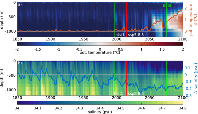
a Hovmoeller plot of the yearly mean potential temperature in Filchner Trough for the historical simulation hist1 and the scenario SSP5-8.5, and the average temperature change (orange) relative to the 1850-1900 mean (gray). The red line marks the transition from historical to scenario simulation. The green lines mark the phase boundaries. b same as a but for salinity.
-
II.
The beginning of the second phase is defined as the point in time when the mean temperature in Filchner Trough rises above the long-term mean of 1850-2014, i.e. when the annual mean temperature in the trough lies above the mean plus the standard deviation from phase I for longer than two consecutive years. Over the course of this phase, temperature in the Filchner Trough is increasingly dominated by pulses of mWDW (Fig. 3a), while salinity in the trough slowly declines (Fig. 3b).
-
III.
The last phase begins when the mean temperature in the trough rises permanently above −1 ∘C. In this state, the trough is mostly filled with mWDW and the seasonal signal has vanished. The mitigation scenario SSP1-2.6 is the only scenario that does not reach this state (Fig. 4, Supplementary Fig. 1).
Fig. 4: Simulated potential temperature evolution in Filchner Trough for four climate scenarios. 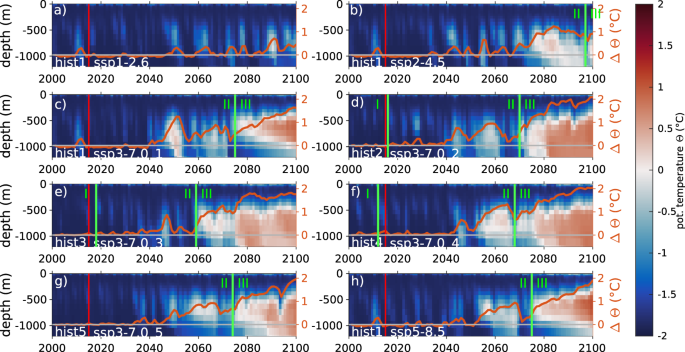
Hovmoeller plots of the yearly mean potential temperature in Filchner Trough from the year 2000 to 2100, with the average temperature change in the Filchner Trough relative to 2000 shown in orange, for the climate scenarios: a SSP1-2.6, b SSP2-4.5, c–g SSP3-7.0 (five ensemble members) and h SSP5-8.5. The vertical red lines divide the timeline into the historical simulations (before 2015) and the future climate scenarios (from 2015 onward). Green lines mark the phase boundaries.


During Phase I, the average temperature in Filchner Trough stays low near −1.8 ∘C and only shows seasonal warming by typically less than 0.25 ∘C relative to the 1850-1900 mean, reaching no higher than −1.5 ∘C (Fig. 4). During Phase II, the average maximum temperature of the current reaching the Filchner Trough over all scenarios is increased to −0.41 ∘C ± 0.36 ∘C (sampled at transect A, see Fig. 2). The longer the pulse lasts, the warmer the water that is registered in the trough, e.g the pulse in hist1 lasting from 2008 to 2012 reaches a peak temperature that is 0.68 ∘C warmer (potential temperature of −0.19 ∘C) compared to 2007 at its core along transect A. Most shorter warm water pulses show a lower temperature than this and remain below the temperature increase of 0.5 ∘C described by Ryan et al.22. All our climate projections show increasing numbers of mWDW pulses entering the Filchner Trough during the second phase (Fig. 4). The frequency of these pulses stays relatively constant until 2050.
In the second half of the 21st century, the multiyear intrusions of mWDW increase in length and frequency depending on the forcing scenario. While SSP1-2.6 remains in Phase II and returns to its DSW-filled state after each pulse (Fig. 4a), the SSP2-4.5 scenario transitions into Phase III during the last four years of the simulation with a warmer state than the SSP1-2.6 but colder than the temperatures reached in SSP3-7.0 or SSP5-8.5 (Fig. 4b). It is unclear if the warm state would be maintained or the trough would return to a colder temperature if the scenario continued beyond the year 2100. In the SSP3-7.0 ensemble and in SSP5-8.5, the trough clearly shifts to a consistently warmer state (Fig. 4c–h). In these two higher-emission climate projections, the Filchner Trough in Phase III stays warm and is filled with mWDW. For this particular aspect, results from the SSP5-8.5 lie within the spread of the SSP3-7.0 ensemble.
The observation of an especially warm and prolonged mWDW presence on the continental shelf during 201722 suggests that the Filchner Trough in reality is either on the brink of transitioning or it has already transitioned into Phase II.
Evaluation of circulation characteristics
Present mean state
A particular feature of our climate model simulations is that for a global coupled climate model, many aspects of the results of the historical simulations for the period 2000-2014 are in remarkably good agreement with observations in key areas around the Filchner Trough (Fig. 5a, Supplementary Fig. 4a, for the definition of key areas see Methods and Supplementary Fig. 9). Due to the high variability of the water mass properties on the continental shelf and the fact that model years in a climate model do not reflect the actual year-to-year evolution, a direct comparison of the model results with hydrographic measurements taken as a snapshot or over a short period of time is difficult. The position and strength of the modeled mWDW current shows a strong interannual variability (Supplementary Fig. 5) that can cover the true variations only with regard to their statistical properties. However, the temperature and salinity distributions in key areas show a similar pattern in the model results as in observations, indicating that the model can reproduce the main features and processes that define the circulation in the Weddell Sea, even without ice shelf cavities (Fig. 5, Supplementary Fig. 4a). The most important water masses and circulation features in the western Weddell Sea, except for Ice Shelf Water (ISW), can be clearly identified. The simulations do not produce ISW due to the absence of ice shelf cavities in the model grid. The coldest water mass in the Filchner Trough has in-situ surface freezing temperature (approx. −1.9 ∘C). However, all other water mass properties compare well with observations even quantitatively (Fig. 5a, Supplementary Fig. 4a).

a Potential temperature in a 15-year average of the ensemble mean of the historical scenario (2000 to 2014) at the sea floor and at sections along 33∘W, 38∘W, 73.8∘S and 76∘S with differences to observational data (flags,33,34,35,36,37). Arrows indicate the slope current of WDW and mWDW flowing along the continental shelf break and onto the shelf. Upper colorbar: standard deviation of difference of model data to observational data in averaged key areas (flag color), lower colorbar: potential temperature along sections and sea floor. b Change in potential temperature in the 15-year average 2086 to 2100 compared to a) in the ensemble mean of SSP3-7.0.
Large-scale circulation features two cyclonic cells forming the Weddell Gyre (Supplementary Fig. 2a) as has been suggested by earlier model studies28. The volume transport of the simulated Weddell Gyre is 46 Sv at the Prime Meridian and thus similar to observational data29,30 (Supplementary Fig. 2b). Transport by the ACC across 60∘W amounts to 170 Sv and is therefore on the high side of observation-based estimates (e.g., 107-161 Sv in Drake Passage31,32). The Antarctic Slope Current transports mWDW with a potential temperature θ > 0 ∘C along the continental slope southward (Fig. 5a). The main current turns west at about 74∘S and follows the continental slope towards the Antarctic Peninsula (Supplementary Fig. 3). A side current branches off and cooler mWDW flows onto the continental shelf east of Filchner Trough and along the trough’s eastern slope, indicated by a warm signature with temperatures between −0.5 ∘C and 0 ∘C on the eastern continental shelf, and approximately −1.5 ∘C over the eastern slope of Filchner Trough (Fig. 5a), similar to the observations described by9. In the 15-year mean, this southern branch can be traced south to 76∘S (Fig. 5a). The simulation reproduces WSDW and WSBW in the Weddell Sea with temperatures between −0.8 ∘C and 0 ∘C, and Antarctic surface water with temperatures below −1.5 ∘C and the lowest salinity values in the central Weddell Sea (S < 34.3; Fig. 5a, Supplementary Fig. 4a).
The ensemble mean of the historical simulation is a close match for observational data in key areas in and around Filchner Trough33,34,35,36,37,38. In the central Filchner Trough (FT), at the Filchner ice shelf front (FIS), on the continental shelf west of the trough (WCS) and off-shore over the continental slope (OS), the mean ensemble temperature deviates by 0.06 ∘C or less from observation data (flags in Fig. 5a). The standard deviation in each of the key region shows that the largest variations in the deviation between model and observations are found at the off-shore location, caused by a varying depth of the ASF. The largest positive temperature bias can be found on the eastern shelf and on the eastern slope of the Filchner Trough, areas that are subject to strong annual and interannual variability due to the varying mWDW flux. This area is 0.36 ± 0.36 ∘C warmer in the model average than in the observations. The bottom salinity of the ensemble mean ranges from 34.33 on the Berkner Shelf to 34.58 in the Filchner Trough and deviates by 0.12 ± 0.06 psu from observations (Supplementary Fig. 4a). The model trough is filled with DSW with a minimum simulated temperature of −1.9 ∘C. Generally, the model results are slightly warmer and fresher on the continental shelf than observational data suggest.
The circulation on the shelf agrees well with observed patterns in most areas outside of the ice shelf cavities9,14. We identify three major areas of dense water overflow: the Filchner Sill, the center of the southern Weddell Sea continental shelf at approx. 47∘W, and north of the Ronne Trough (Supplementary Fig. 3). Because of the lack of an ice shelf cavity, High Salinity Shelf Water/DSW produced in the Ronne Trough flows northward towards the Antarctic Peninsula and not through the cavity towards the Filchner Trough39,40.
Seasonality
Phase I (as defined above) is characterized by a seasonal influx of varying length of mWDW into Filchner Trough, which increases the mean temperature in the trough during winter. The model results show the main transport of mWDW into the Filchner Trough taking place via the continental shelf east of the Filchner Trough (Fig. 5a, Supplementary Fig. 3), while occasionally smaller currents enter the trough over the central and western depression (Supplementary Fig. 5), reproducing observed patterns13,14,41. The warm water takes several months to travel from the slope southward before going west, down the slope into the trough.
The seasonal influx of mWDW onto the shelf east of Filchner Trough and along the eastern slope of the trough was reported to be the strongest during February to June and weaker during the spring and summer months13,18,19,42. Mooring data (AWI254) from 31.5∘W 76∘S shows the warming onset caused by mWDW during late March, early April (Fig. 6a,36). However, Ryan et al.18 reported the presence of mWDW at 31∘W already starting in January. To compare the model output to the mooring observations, we compute an area-weighted temperature average over the area outlined in Fig. 2. We see similar behaviour in the simulation as in the observations (Fig. 6b). MWDW generally starts to arrive at 76∘S during March, however as the examples show, the onset can vary by several months and in strength. The timing of the maximum temperature varies between February and June18,22, and so does the timing in the simulations.

a Mooring data from January 2016 to December 201636, b Model output for the area outlined in green in Fig. 2 for 2002–2004. The red lines indicate the temperature averaged between 410 m and 520 m. In a a five-days running mean was applied to the vertically averaged temperature data. The temperature and depth scales are valid for both panels.
During April to August the model results show an intensification of the northbound transport of DSW along the western slope of the Filchner Trough (Fig. 7), caused by a higher sea ice production over Berkner Shelf in autumn and winter. Morrison et al.43 proposed that northward DSW transport in a canyon or trough leads to a gradient in sea surface height due to the replacement of less dense water along the western canyon slope with DSW. This creates a barotropic pressure gradient which drives more lighter AASW and mWDW from the northeast into the trough43(their schematic in Fig. 5A). Given that our model results show similar characteristics in the density distribution across the Filchner Trough and a difference in sea surface height between eastern and western slope of the trough (Fig. 7), we conclude that the mechanism proposed by Morrison et al.43 offers a plausible explanation for the timing and structure of the seasonal mWDW inflow both in the model and in reality. The intensification of the north-bound transport and the simultaneously increased presence of denser water in autumn strengthen the pressure gradient across the trough and bring more mWDW into the trough, leading to the observed seasonal increase in temperature.

The line plot in blue shows the sea surface elevation (ssh in m). The panel below shows the meridional velocity component (m/s) as background color, with isopycnals (black: 27.7 kg/m3, dotted: 27.6 kg/m3, dashed: 27.5 kg/m3, gray: <27.5 kg/m3) for the simulated monthly means of 2000-2014. Positive numbers for the velocity (i.e. reddish colors) indicate northward flow.
As an additional component, the depth of the thermocline at the continental slope also shows a weak seasonal oscillation. It rises during spring and summer, and deepens during autumn and winter. This facilitates the flow of mWDW onto the continental shelf during summer, when the thermocline is at its shallowest. The mWDW then takes two to three months to reach the Filchner Trough.
Future evolution
During the climate projections for the 21st century, the characteristics of the water mass filling the Filchner Trough change significantly. Some of these changes can already be observed at the end of the historical simulations when the Filchner Trough reaches Phase II. Causes for these changes can be found in the local sea ice formation as well as upstream, and in the position and temperature of the Antarctic Slope Current. The mechanism behind the increased presence of mWDW on the shelf is different from the one responsible for the seasonal variation. It will be described in the following.
Changes in Filchner Trough
In the emission scenario SSP3-7.0, the mean water temperature in Filchner Trough is warmer by approx. 2 ∘C (Fig. 8a) and saltier by less than 0.2 psu (Supplementary Figs. 1c-g and 4b) by the end of the century, showing the permanent presence of mWDW. Salinity of near-surface water on the continental shelf, however, has decreased by up to 0.8 psu, following a decrease in sea ice formation (Fig. 8a). Further changes occur along the continental slope, where the slope current warms by up to 1 ∘C (Figs. 5b and 8a). The high-emission scenario SSP5-8.5 shows similar warming patterns with an even further increase in bottom temperature on the continental shelf at the Berkner Bank and north of the Ronne Trough (temperature anomaly between 1.5 ∘C and 1.8 ∘C). The mitigation scenarios SSP1-2.6 and SSP2-4.5 show a similar distribution of warming water, but the temperature rise in Filchner Trough is limited to 1 ∘C or less. The average salinity in Filchner Trough increases in SSP3-7.0 and SSP5-8.5 where mWDW, with a higher salinity than the fresher DSW, is registered permanently in the Filchner Trough (Fig. 3b, Supplementary Figs. 1c-h and 4b).

a 10-year running mean of yearly mean temperature and sea ice formation rate at the slope at S70 (Fig. 2) and in the Filchner Trough for SSP1-2.6 and the ensemble mean of SSP3-7.0. Mean temperature (hues of red) was calculated for Filchner Trough and the bottom layer at the slope at S70. Mean sea ice formation rate (hues of blue) was calculated for Filchner Trough and at S70. b Depth of the thermocline at the shelf break (black) and area average of surface stress curl (gray) at S70 in SSP1-2.6 and the ensemble mean of SSP3-7.0.
In all scenarios, the increase of the average temperature in the Filchner Trough accelerates during Phase II. During the 2030s, the average temperature in the trough for the ensemble mean of SSP3-7.0 rises from −1.75 ∘C to −1.6 ∘C (thick red line in Fig. 8a), while the temperature in SSP1-2.6 (thin red line in Fig. 8a) decreases slightly. Starting from 2040, the average temperature in the Filchner Trough in SSP3-7.0 rises quickly and reaches 0.3∘C in 2100, 2 ∘C warmer compared to 2000. This goes hand in hand with a strong decrease of sea-ice formation in the area of Filchner Trough beginning in the early 2030s (thick dark blue line in Fig. 8a). In 2000, the model produces on average approx. 2.4 m/yr of sea ice at the Filchner Trough. Towards the end of the century, this reduces to 1.6 m/yr. Changes in the mean temperature in Filchner Trough in the lowest-emission scenario SSP1-2.6 are comparably small. Compared to 2000, mean temperature in SSP1-2.6 increases by 0.15 ∘C until 2050 similar to the higher-emission scenarios, but in contrast to those, the temperature rises only by 0.5 ∘C compared to 2000 until 2100. Sea ice formation in the Filchner Trough area does not decrease at all in SSP1-2.6 (thin dark blue line in Fig. 8a).
Changes upstream of Filchner Trough
While the temperature in Filchner Trough begins to rise in the 2030s and is scenario-sensitive with regard to magnitude and timing of the warming, the temperature of the slope current upstream of the Filchner Trough transporting mWDW towards the southern continental shelf increases over the whole simulation, independent of the climate scenario (orange lines in Fig. 8a). In all four scenarios, the average temperature at the bottom of the slope current at about 70∘S increases from −0.45 ∘C in 2000 to −0.1 ∘C in 2100 (0.03∘C per decade), which is a smaller trend than the CDW warming of approx. 0.05 ∘C per decade that was observed in the Weddell Sea from 1980 to 201020. However, the shoaling of the thermocline is scenario-dependent with 10 m per decade in SSP3-7.0 and 7 m per decade in SSP1-2.6 (black lines in Fig. 8c).
The shoaling of the thermocline is consistent with observations, but the rate is lower than the 30 m per decade suggested from observations in the Weddell Sea20. The change in depth of the thermocline relates directly to the reduced down-welling at the continental slope (more negative average surface stress curl, gray line in Fig. 8c), caused by weakening Easterlies and a southward displacement of the transition zone between Westerlies and Easterlies above the Weddell Sea during January to March (Supplementary Fig. 6a). The wind field above the Weddell Sea gains strength during July to August (Supplementary Fig. 6b), while during January to March, the 15-year average wind speed above the continental shelf east of 15∘W is reduced by 0.5 m/s between 2000–2014 and 2086–2100.
The decreasing sea ice formation over the Filchner Sill and growing differences between the climate projections become visible in the sea ice extent during the second half of the 21st century (Figs. 8 and 9). Until 2050, the spread between the different scenarios (Fig. 9a, b) is not larger than the spread between the different ensemble members for the SSP3-7.0 scenario (Fig. 9c, d).

a March and b September sea ice extent in the Weddell Sea, with results from the historical simulations and SSP3-7.0 being averaged over all five ensemble members (line plots). Shading in the background of a and b shows sea ice thickness difference between the 15-year averages of hist1 (2000-2014) and SSP5-8.5 (2086-2100). c and d same as a and b, but all ensemble members of SSP3-7.0 shown individually.
In SSP5-8.5, summer sea ice shrinks until only a small area in the southwestern Weddell Sea remains ice-covered. Average summer sea ice thickness reduces in the Weddell Sea by up to 1.3 m. In contrast to the other scenarios, SSP1-2.6 shows no further area loss in summer sea ice after 2050 (Fig. 9a). While the sea ice extent in the southeastern Weddell Sea reaches 73∘S for 2000 to 2014, ice coverage reduces with increasingly warmer climate until the sea-ice cover in the southern Weddell Sea is confined in summer to south of 74∘S by 2050 (Fig. 9). Summer sea ice extent reduces in SSP5-8.5 by ≈76% in the Weddell Sea from 3.69 × 10⁶ km2 to 0.88 × 10⁶ km2. The sea ice opens first along the eastern coast of the Weddell Sea, clearing the Filchner Trough of summer sea ice. By the end of the projected time period, the Filchner Trough is only partly ice-covered (SSP1-2.6, SSP2-4.5) or completely ice-free in summer (SSP3-7.0, SSP5-8.5). The winter sea ice extent by contrast shows far less variability. The largest changes in September sea ice occur in SSP5-8.5 towards the end of the century. But even though the sea ice extends as far north during the period of 2086 to 2100 as it did in the beginning of the simulation, sea ice freezing rates during winter are much lower, causing a decrease in sea ice thickness by up to 1 m in September compared to the historical period and reducing the amount of sea ice melting in summer.
Changes of seasonality
Over the course of Phase II after 2050, the seasonal variation in Filchner Trough temperature decreases more or less strongly, depending on the climate scenario (Fig. 10). The weaker seasonal signal is particularly pronounced in SSP3-7.0 and SSP5-8.5 (Fig. 10), but it can also be found during a brief period in 2089 and 2090 in SSP1-2.6 (Fig. 10a). The connection of the seasonality and the local sea ice formation becomes only clear when the sea ice formation is particularly low. In SSP5-8.5, this is the case 2050 onward Fig. 10b). Before that, a decrease in sea ice formation rate does not coincide with lower seasonality. The permanent loss of the seasonal signal marks the transition from Phase II to Phase III as defined above.

a for SSP1-2.6 and b for SSP5-8.5. Red (blue) dots depict the difference between the temporal and spatial maximum (minimum) of the area to the temporal mean of the spatial maximum along the transect in the Filchner Trough (Fig. 8). The bars illustrate the seasonal variation. The green line represents the sea ice formation in the Filchner Trough.
Discussion and Conclusions
The present study shows that over the course of this century strong changes in the hydrography of the Filchner Trough are imminent. Already in the present climate, warm water pulses reach the Filchner ice shelf front both in the model simulations presented here and according to observations19,22,41. The comparability between the historical simulations and observations gives confidence into our model projections for the future climate evolution.
It should be noted that in the current simulations ice shelf cavities are not considered. Previous specialized ocean model simulations with ice shelf cavities (e.g.8,12) showed the same three modes as our CMIP6 simulations: seasonal warm water only in Phase I, intermittent warm water pulses in Phase II (and in present-day climate), and persistent warm water in Phase III, occurring in future climate scenarios with strong emission of greenhouse gases. This implies that cavity circulation is not a critical component in triggering the simulated changes in the Filchner Trough hydrography. Instead, reduced sea ice formation and changing wind fields play a major role. This concurs with the results from Naughten et al.12, who showed that the intrusion of mWDW into the ice shelf cavity can only happen after the density on the continental shelf has reduced to a critical value, therefore sea ice formation on the shelf has a larger direct impact on the mWDW flux than any processes below the ice shelves.
The amount of heat that reaches the Filchner Trough depends on two factors: The amount of southward transport of (m)WDW onto the continental shelf and the grade of modification of the WDW by vertical mixing through DSW formation (Supplementary Fig. 7). Of these two, the first factor depends on the density gradient between the continental shelf waters and the slope current, and on the depth of the ASF at the continental slope. The grade of modification depends on the depth and intensity of convection and thus primarily on the rate of sea ice formation. However, DSW formation also influences the density gradient at the shelf edge and thus the on-shelf transport. A clear separation between the two processes is therefore not possible, but we conclude that sea ice formation plays a dominant role in governing the mWDW transport into the trough.
As a caveat, we note that in reality density of the water masses on the continental shelf is clearly influenced by the ISW outflow from under the ice shelf, which may have an impact on the timing of the regime shift we find in the high-emission scenarios. Given that ice shelf melting is a source of freshwater, it could be argued that adding ice shelves to our simulation would reduce the density of water masses on the continental shelf, potentially accelerating the regime shift towards a warm continental shelf. But then, given the very low temperatures of ISW, the mixing product of ISW and (m)WDW is a very dense water mass known to contribute to WSBW formation. A denser watermass on the shelf would potentially delay the regime shift. Which of these effects dominates is not obvious to us, but we note that they counteract each other, which mitigates a potential bias caused by the missing ice shelves in our simulations. A similar case can be made for the fact that we neglect the freshwater input from the ice shelves in the eastern Weddell Sea, upstream of Filchner Trough. In the presence of these ice shelf cavities, we would expect a stronger stratification over the shelf break, strengthening the Antarctic Slope Front (ASF) and reducing the mWDW flux onto the shelf. However, increased freshening of the shelf water masses might also a) cause baroclinic instabilities and thus an uplift of the thermocline44,45 and b) reduce the density gradient between the continental shelf and the Filchner-Ronne ice shelf cavity. Whether the ice shelves in the eastern Weddell Sea rather facilitate or inhibit the flow of warm water into the Filchner Trough is therefore not clear and needs to be addressed in a follow-up study.
While sea ice is the main driver behind the variations of mWDW transport onto the shelf and into the Filchner Trough, the model underestimates summer sea ice extent in the Antarctic, but slightly overestimates the winter sea ice extent25. The smaller sea ice area in summer might increase heat uptake during the warmest part of the year, creating a feedback loop of warmer sea surface temperatures decreasing and delaying sea ice formation. This would decrease the modification of WDW so that water closer in temperature to WDW reaches the trough and might cause an overestimation of simulated warming in Filchner Trough in SSP3-7.0 and SSP5-8.5. On the other hand, a reduced summer sea ice extent leads to additional sea ice formation in fall and thus additional salt input (similarly to the processes in coastal polynyas), potentially compensating or even overcompensating for the effect of too strong heat uptake in summer.
Despite the caveats outlined above, and given that the sign of the bias each of them could create is not obvious in all cases, we are confident that our main findings are robust. We find a decrease of ASF depth over the course of the high-emission scenario simulations that might facilitate the warm water influx to the Filchner Trough, notably in combination with pronounced density changes on the shelf. The receding sea ice and reduced freezing rates on the continental shelf in a warming climate cause the DSW in the Filchner Trough to freshen, reducing the intensity of vertical mixing between DSW and the underlying mWDW. A decline in density on the shelf weakens the density gradient at the continental shelf break and allows mWDW to flow into the trough11,46. This effect is especially large in the high-emission scenarios. Because the sea ice formation mostly depends on atmospheric processes, the differences in forcing in the SSP scenarios heavily impact changes in sea ice formation rates in the Weddell Sea.
The uplift of the ASF above the continental shelf in turn is caused by changing wind fields, reducing downwelling at the continental slope by lessening the coastward Ekman transport by easterly winds from January to March. Stronger westerly winds above the central Weddell Sea and a southward shift of the transition zone between Westerlies and Easterlies further decrease areas of downwelling along the coast. The wind above the continental shelf east and north of the Filchner Trough has a much higher westward component during the summer months of the high-emission scenarios SSP3-7.0 and SSP5-8.5 in 2086-2100 compared to 2000-2014. Even though the lower sea ice concentration in the high emission scenarios should increase the wind stress on the ocean, the effect is balanced by weaker wind during summer, a northwest-going wind field during the following months promoting upwelling along the coast, and reduced erosion of mWDW on the continental shelf by sea ice formation during the following autumn and winter.
There is a clear seasonality in the mWDW influx both in our model simulations and according to Darelius et al.19 as well as Ryan et al.18,22. While Ryan et al.22 attribute the seasonal inflow of mWDW to an inflow of freshened shelf waters from the coast of Dronning Maud Land, causing baroclinic instabilities and lifting the thermocline, we mainly attribute this seasonal inflow to the autumn maximum in local sea-ice production. According to Morrison et al.43, sea ice formation causes increased DSW production and northbound transport in the Filchner Trough and establishes a pressure gradient across the trough that fosters the near-surface inflow of mWDW.
The sea ice decrease towards the end of the century in the high-emission scenarios, especially in thickness, is caused by the increased heat flux from the atmosphere. Higher CO2-concentration in the atmosphere escalates the greenhouse gas effect and changes the heat flux in the western Weddell Sea from net heat loss to heat gain (Supplementary Fig. 8), warming the ocean and reducing sea ice formation. The southward displacement of the wind belt, stronger variability of the wind fields and strengthening of the wind field increase the off-shore sea ice transport and cause stronger sea ice deformation, which could potentially increase sea ice formation rates. However, weakening easterlies above the continental shelf in the eastern Weddell Sea during summer and a stronger heat flux towards the ocean counteract this effect, increase sea surface temperature and lead to thinning of the sea ice in the Weddell Sea. The driving factor behind the reduced sea ice formation is therefore not the wind but the increased heat flux at the surface during the climate scenarios.
Towards the end of the century, the general decrease in sea ice formation in the simulations leads to a decrease in the strength of the seasonal signal of the mWDW. The reduction of the density of the DSW outflow along the western slope of the Filchner Trough causes a weakening of the across-trough pressure gradient during winter. The reduced sea ice production weakens the convection in winter, when in the present state the flow of mWDW is eroded by deep vertical mixing triggered by sea ice formation. Together with the uplift of the thermocline above the continental shelf break (Fig. 8b), the weaker winds during the following summer months prolong the time where mWDW intrusions are possible, leading to a year-round presence of mWDW on the shelf. A regime shift occurs when DSW production in the Filchner Trough and surrounding continental shelf is not sufficient anymore to erode the inflow of mWDW into the trough during winter and spring. This point is reached between 2070 and 2080 in the high-emission scenarios SSP3-7.0 and SSP5-8.5, confirming the timing suggested by previous numerical model simulations with different, prescribed atmospheric forcing8,10,11,23,46.
An important finding in our model results is that sea ice formation and extent, temperature in Filchner Trough and depth of the ASF all really start to differentiate between the different SSP scenarios in the 2040s. The slope current temperature even does not vary between the scenarios at all until 2100. This indicates that any endeavors to change the course of the current and future climate development will only start to show results in 20 to 30 years or later. If we as humanity do not change our habit of emitting greenhouse gases soon, the pulses of warm water reaching the continental shelf could be replaced by a permanent warm water flow (according to the strong emission scenarios SSP3-7.0 and SSP5-8.5). The presence of this warm water is bound to increase ice shelf basal melt, leading to a thinning of the ice shelf, a reduced buttressing to the ice flow, and additional sea-level rise. If a marine ice sheet instability is triggered, this process is self-sustained and can accelerate even if the original perturbation (here: the warm water inflow) is removed. If we do make the effort to restrict greenhouse gas emissions substantially, we could preserve the state of intermittent pulses of warm water reaching the continental shelf and possibly restrict ice shelf melting. According to our findings, a regime shift towards a warm cavity under Filchner Ronne Ice Shelf with strongly increased basal melt rates and an increased contribution to global sea-level rise can only be sustainably avoided by reaching the 2 ∘C (SSP1-2.6) climate goal. With the SSP2-4.5 scenario, restricting the global warming to 3 ∘C, no regime shift to a permanent warm inflow occurs in our simulation until 2100, but the water in Filchner Trough still warms by 1 ∘C in this scenario. Whether this may still trigger a marine ice sheet instability or leads to the crossing of any tipping point with a large impact on global sea-level rise is a topic of ongoing research.
Methods
Model
The simulations were performed with the AWI Climate Model (AWI-CM). It is a coupled model consisting of the Finite Element Sea ice-Ocean Model (FESOM v.1.4) and the atmospheric model ECHAM6, developed by the Max Planck Institute for Meteorology in Hamburg. The components are coupled via the OASIS3-MCT coupler. The ocean-sea ice model FESOM uses unstructured meshes which allow for a variable grid resolution in highly dynamic regions. More information on FESOM is provided by Wang et al.47. ECHAM6 is a spectral atmospheric model48, which was used without any additional modifications or tuning. For more information on the performance of AWI-CM see ref. 25,49,50.
The ocean grid ‘MR’ used in the simulations has a medium resolution with a resolution distribution following the strategy proposed by Sein et al.51,52. The resolution is locally increased in areas of high sea surface height variability derived from satellite data and ranges between 8 km and 80 km53,54,55. The horizontal resolution in the Weddell Sea varies between 12 km and 40 km. While eddy transport is not resolved, the eddy parameterization has been proven to work well with the mesh resolution used here, producing isopycnals very similar to atlas data56. The grid has 46 unevenly spaced layers with a minimum layer thickness of 10 m near the surface and a maximum spacing of 250 m at the bottom. The mesh does not include ice shelf cavities. Tides are not explicitly calculated, but the effect of barotropic tides is included in the calculation of the Richardson number as proposed by47,57.
The atmosphere component uses the resolution of T127L95. T127 stands for the spectral truncation of wave number 127, which corresponds to approximately 100 km horizontal resolution in the tropics and higher resolution towards the poles. The atmosphere has 95 unevenly spaced layers with lower spacing of the levels near the surface and wider spacing towards the top of the atmosphere.
AWI-CM participated in the sixth round of the Coupled Model Intercomparison Project (CMIP6). The simulations include a historical forcing simulation and four subsequent climate simulations with forcing derived from Shared Socioeconomic Pathways (SSP)24,27. For the historical scenario, five ensemble members were simulated. Preceding the start of the historical simulations a spin-up period was computed. This includes 10 years ocean-only simulation, 500 years of pre-industrial control spin-up with constant pre-industrial forcing and 500 years of piControl from which the historical simulations were branched off in the years 150 (hist1), 175 (hist2), 200 (hist3), 225 (hist4) and 250 (hist5). The future climate simulations were performed for the scenarios SSP1-2.6, SSP2-4.5, SSP3-7.0 and SSP5-8.5. Only SSP3-7.0 has 5 ensemble members25. The scenarios SSP1-2.6, SSP2-4.5, SSP5-8.5 and the first member of SSP3-7.0 started from 2014 of hist1. The other ensemble members 2 to 5 of SSP3-7.0 were branched off the corresponding historical ensemble members.
Validation
To validate the model results we use a data set that has been compiled from in-situ observations by Mathias v. Caspel (pers. comm. 2022). The data set includes salinity and potential temperature from the years 199533, 201334,38, 201635,36 and 201837 at depths between 100 m and 1200 m in different areas of the southern Weddell Sea. We choose six key areas as shown in Supplementary Fig. 9 for validation: central Filchner Trough (FT), Filchner Sill (FS), the Filchner Trough at the Filchner ice shelf edge (FIS), the continental shelf east of the Filchner Trough (ECS), the continental shelf west of the Filchner Trough (WCS), and at 74∘S off-shore of the continental shelf (OS). The locations were chosen to be representative for specific water masses.
We interpolated the model results vertically for temperature and salinity onto the greatest depth at each observation location, and interpolated between the three nearest horizontal grid points. The resulting temperature and salinity values were then compared to the observational data. From these differences we calculated the average difference and standard deviation in each key area, displayed in the flags of Fig. 5a and Supplementary Fig. 4a.
Calculation of diagnostic properties
The ASF is defined as the boundary between the continental shelf water masses and the denser and warmer (m)WDW of the slope current. To identify this boundary, we use the thermocline and pycnocline between the two water masses. The model data was selected for the area around 70∘S as depicted in Fig. 8b. For each mesh layer, the data was then averaged in twelve equidistant bins approximately parallel to the coastline. The temperature and density gradients were calculated between the mesh layers, and the depth with the highest gradient between bins selected as the depth of the ASF. The temperature at the slope was calculated by averaging the temperature of the bottom bins. As this includes the surface layer and the bottom temperature at greater depth, the result underestimates the real slope current temperature.
To calculate a measure for the seasonal variability of the mWDW influx into the Filchner Trough, we choose section A approximately perpendicular to the main axis of the Filchner Trough, ranging from 75.95∘S 37.31∘W to 76.54∘S 30.66∘W (Fig. 2). Along this profile, the spatial maximum of the monthly mean temperature was selected. The seasonal variability was then computed as the difference between the temporal maximum and temporal minimum of the spatial maximum temperature per year.
Data availability
All data are available on the Earth System Grid Federation (ESGF): http://esgf-data.dkrz.de/search/cmip6-dkrz/?mip_era=CMIP6&activity_id=CMIP&institution_id=AWI&source_id=AWI-CM-1-1-MR58. A processed minimum data set can be accessed under https://doi.org/10.5281/zenodo.10552405.
Code availability
The code for AWI-CM can be accessed from the esm-tool at https://github.com/esm-tools/esm_tools after registration with the MPI-ESM user forum (last access 16.09.2022). The Matlab codes used for the analysis of the model output will be made available upon request to the corresponding author.
References
Fretwell, P. et al. Bedmap2: improved ice bed, surface and thickness datasets for antarctica. Cryosphere 7, 375–393 (2013).
The IMBIE team. Mass balance of the antarctic ice sheet from 1992 to 2017. Nature 558, 219–222 (2018).
DeConto, R. & Pollard, D. Contribution of antarctica to past and future sea-level rise. Nature 531, 591–597 (2016).
Shepherd, A. et al. A reconciled estimate of ice-sheet mass balance. Science 338, 1183–1189 (2012).
Mouginot, J., Rginot, E. & Scheuchl, B. Sustained increase in ice discharge form the amundsen sea embayment, west antarctica, from 1973 to 2013. Geophys. Res. Lett. 41, 1576–1584 (2014).
Arneborg, L., Wåhlin, A. K., Björk, G., Liljebladh, B. & Orsi, A. H. Persistent inflow of warm wate ronto the central amundsen shelf. Nat. Geosci. 5, 876–880 (2012).
Jacobs, S. et al. The amundsen sea and the antarctic ice sheet. Oceanography 25, 154–163 (2012).
Hellmer, H. H., Kauker, F., Timmermann, R., Determann, J. & Rae, J. Twenty-first-century warming of a large antarctic ice-shelf cavity by a redirected coastal current. Nature 485, 225–228 (2012).
Foldvik, A., Gammelsrø d, T. & Torresen, T. Circulation and water masses on the southern weddell sea shelf. Oceanol. Antarctic Continent. Shelf 43, 5–20 (1985).
Timmermann, R. & Goeller, S. Response to filchner-ronne ice shelf cavity warming in a coupled ocean-ice sheet model - part 1: The ocean perspective. Ocean Sci. 13, 765–776 (2017).
Timmermann, R. & Hellmer, H. H. Southern ocean warming and icreased ice shelf basal melting in the twenty-first and twenty-second centuries based on coupled ice-ocean finite-element modelling. Ocean Dynam. 63, 1011–1026 (2013).
Naughten, K. A. et al. Two-timescale response of a large antarctic ice shelf to climate change. Nat. Commun. 12, 1–10 (2021).
Årthun, M., Nicholls, K.-W., Makinson, K., Fedak, M.-A. & Boehme, L. Seasonal inflow of warm water onto the southern weddell sea continental shelf, antarctica. Geophys. Res. Lett. 39, 2–7 (2012).
Nicholls, K., Østerhus, S., Makinson, K., Gammelsrød, T. & Fahrbach, E. Ice-ocean processes over the continental shelf of the southern weddell sea, antarctica: A review. Rev. Geophys. 47, 1–23 (2009).
Nicholls, K. W., Boehme, L., Biuw, M. & Fedak, M. A. Wintertime ocean conditions over the southern weddell sea continental shelf, antarctica. Geophys. Res. Lett. 35, L21605 (2008).
Foldvik, A. et al. Ice shelf water overflow and bottom water formation in the southern weddell sea. J. Geophys. Res. 109, C02015 (2004).
Naveira Garabato, A. C., McDonagh, E. L., Stevens, D. P., Heywood, K. J. & Sanders, R. J. On the export of antarctic bottom water from the weddell sea. Deep-Sea Res. Part II: Topical Studies Oceanography 49, 4715–4742 (2002).
Ryan, S., Hattermann, T., Darelius, E. & Schröder, M. Seasonal cycle of hydrography on the eastern shelf of the filchner trough, weddell sea, antarctica. J. Geophys. Res.: Oceans 122, 6437–6453 (2017).
Darelius, E., Fer, I. & Nicholls, K.-W. Observed vulnerability of filchner-ronne ice shelf to wind-driven inflow of warm deep water. Nat. Commun. 7, 1–7 (2016).
Schmidtko, S., Heywood, K. J., Thompson, A. F. & Aoki, S. Multidecadal warming of antarctic waters. Science 346, 1227–1232 (2014).
Turner, J. et al. Recent decrease of summer sea ice in the weddell sea, antarctica. Geophys. Res. Lett. 47, e2020GL087127 (2020).
Ryan, S. et al. Exceptionally warm and prolonged flow of warm deep water toward the filchner-ronne ice shelf in 2017. Geophys. Res. Lett. 47, 1–10 (2020).
Hellmer, H. H., Kauker, F., Timmermann, R. & Hattermann, T. The fate of the southern weddell sea continental shelf in a warming climate. J. Clim. 30, 4337–4350 (2017).
Eyring, V. et al. Overview of the coupled model intercomparison project phase 6 (cmip6) experimental design and organization. Geosci. Model Dev. 9, 1937–1958 (2016).
Semmler, T. et al. Simulations for cmip6 with the awi climate model awi-cm-1-1. J. Adv. Model. Earth Syst. 12, 1–34 (2020).
O’Neill, B. C. et al. The scenario model intercomparison project (scenariomip) for cmip6. Geosci Model Dev. 9, 3461–3482 (2016).
Meinshausen, M. et al. The shared socio-economic pathway (ssp) greenhouse gas concentrations and their extensions to 2500. Geosci. Model Dev. 13, 3571–3605 (2020).
Beckmann, A., Hellmer, H. H. & Timmermann, R. A numerical model of the weddell sea: Large-scale circulation and water mass distribution. J. Geophys. Res. 10, 375–391 (1999).
Klatt, O., Fahrbach, E., Hoppema, M. & Rohardt, G. The transport of the weddell gyre across the prime meridian. Deep-Sea Res. Part II 52, 513–528 (2005).
Reeve, K. A., Boebel, O., Strass, V., Kanzow, T. & Gerdes, R. Horizontal circulation and volume transports in the weddell gyre derived from arge float data. Progress Oceanograp. 175, 263–283 (2019).
Renault, A., Provost, C., Sennéchael, N., Barré, N. & Kartavtseff, A. Two full-depth velocity sections in the drake passage in 2006 - transport estimates. Deep-Sea Res. Part II 58, 2572–2591 (2011).
Koenig, Z., Provost, C., Ferrari, R., Sennéchael, N. & Rio, M.-H. Volume transport of the antarctic circumpolar current: Production and validation of a 20 year long time series obtained from in situ and satellite observations. J. Geophys. Res.: Oceans 119, 5407–5433 (2014).
Schröder, M. Physical oceanography during polarstern cruise ant-xii/3 https://doi.org/10.1594/PANGAEA.742581 (2010).
Schröder, M. & Wisotzki, A. Physical oceanography during polarstern cruise ps82 (ant-xxix/9) https://doi.org/10.1594/PANGAEA.833299 (2014).
Schröder, M., Ryan, S. & Wisotzki, A. Physical oceanography during polarstern cruise ps96 (ant-xxxi/2 frosn) https://doi.org/10.1594/PANGAEA.859040 (2016).
Schröoder, M., Ryan, S. & Wisotzki, A. Physical oceanography and current meter data from mooring awi254-2 https://doi.org/10.1594/PANGAEA.903317 (2019).
Janout, M. A., Hellmer, H. H., Schröoder, M. & Wisotzki, A. Physical oceanography during polarstern cruise ps111 (ant-xxxiii/2) https://doi.org/10.1594/PANGAEA.897280 (2019).
Darelius, E. & Fer, I. Physical oceanography from ctd in the filchner depression (weddell sea, antarctica) during ernest shackleton cruise es060 https://doi.org/10.1594/PANGAEA.846962 (2015).
Foldvik, A. & Gammelsrød, T. Notes on southern ocean hydrography, sea-ice and bottom water formation. Palaeograp. Palaeoclimatol. Palaeoecol. 67, 3–17 (1988).
Nicholls, K. W., Østerhus, S., Makinson, K. & Johnson, M. R. Oceanographic conditions south of berkner island, beneath filchner-ronne ice shelf, antarctica. J. Geophys Res. 106, 11481–11492 (2001).
Janout, M. et al. Fris revisited in 2018: On the circulation and water masses at the filchner and ronne ice shelves in the southern weddell sea. J. Geophys. Res.: Oceans 126, e2021JC017269 (2021).
Darelius, E. et al. On the seasonal signal of the filchner overflow, weddell sea, antarctica. J. Phys Oceanograp. 44, 1230–1243 (2014).
Morrison, A. K., Hogg, A. M., England, M. H. & Spence, P. Warm circumpolar deep water transport toward antarctica driven by local dense water export in canyons. Sci. Adv. 6, eaav2516 (2020).
Hatterman, T. Antarctic thermocline dynamics along a narrow shelf with easterly winds. J. Phys Oceanograp. 48, 2419–2443 (2018).
Nøst, O. et al. Eddy overturning of the antarctic slope front controls glacial melting in the eastern weddell sea. J. Geophys. Res. 116, 1–17 (2011).
Daae, K. et al. Necessary conditions for warm inflow toward the filchner ice shelf, weddell sea. Geophys. Res. Lett. 47, e2020GL089237 (2020).
Wang, Q. et al. The finite element sea ice-ocean model (fesom) v.1.4: Formulation of an ocean general circulation model. Geosci. Model Dev. 7, 663–693 (2014).
Stevens, B. et al. Atmospheric component of the mpi-m earth system model: Echam6. J. Adv. Model. Earth Syst. 5, 146–172 (2013).
Sidorenko, D. et al. Towards multi-resolution global climate modeling with echam6-fesom. part i: model formulation and mean climate. Clim. Dynam. 44, 757–780 (2015).
Rackow, T. et al. Towards multi-resolution global climate modeling with echam6-fesom. part ii: climate variability. Clim. Dynam. 50, 2369–2394 (2018).
Sein, D. V. et al. Designing variable ocean model resolution based on the observed ocean variability. J. Adv. Model Earth Syst. 8, 904–916 (2016).
Sein, D. V. et al. Ocean modeling on a mesh with resolution following the local rossby radius. J. Adv. Model. Earth Syst. 9, 2601–2614 (2017).
Rackow, T. et al. Sensitivity of deep ocean biases to horizontal resolution in prototype cmip6 simulations with awi-cm1.0. Geosci Model Dev. Discuss. 3, 1–25 (2018).
Sein, D. V. et al. The relative influence of atmospheric and oceanic model resolution on the circulation of the north atlantic ocean in a coupled climate model. J. Adv. Model. Earth Syst. 10, 2026–2041 (2018).
de la Vara, A. et al. On the impact of atmospheric vs oceanic resolutions on the representation of the sea surface temperature in the south eastern tropical atlantic. Clim. Dyna. 54, 4733–4757 (2020).
Rackow, T. et al. Sensitivity of deep ocean biases to horizontal resolution in prototype cmip6 simulations with awi-cm1.0. Geosci. Model Dev. 12, 2635–2656 (2019).
Lee, H. C., Rosati, A. & Spelman, M. J. Barotropic tidal mixing effects in a coupled climate model: oceanic conditions in the northern atlantic. Ocean Model. 11, 464–477 (2006).
Semmler, T. et al. Awi awi-cm 1.1 mr model output prepared for cmip6 cmip. earth system grid federation https://doi.org/10.22033/esgf/cmip6.359 (2018).
Acknowledgements
This work was funded by Deutsche Forschungsgemeinschaft SPP 1158 under grants SE2901/2, HE2740/33 and TI296/9. AWI-CM computing time was provided by DKRZ. The research was also supported by the European Union’s Horizon 2020 research and innovation program under grant agreement no. 820575 (TiPACCs). We thank M. van Caspel for providing the data for the hydrographic validation. Thanks also go to Günther Heinemann, Rolf Zentek, Cara Nissen, Thomas Jung, Hartmut Hellmer and Svein Østerhus for the scientific discourse. We acknowledge support by the Open Access Publication Funds of Alfred-Wegener-Institut Helmholtz-Zentrum für Polar- und Meeresforschung.
Funding
Open Access funding enabled and organized by Projekt DEAL.
Author information
Authors and Affiliations
Contributions
TS ran the AWI-CM simulations. VT conducted the analyses and prepared the figures. VT, TS and RT contributed to the interpretation of the results and writing of the manuscript.
Corresponding author
Ethics declarations
Competing interests
The authors declare no competing interests.
Peer review
Peer review information
: Communications Earth & Environment thanks the anonymous reviewers for their contribution to the peer review of this work. Primary Handling Editor: Aliénor Lavergne. A peer review file is available.
Additional information
Publisher’s note Springer Nature remains neutral with regard to jurisdictional claims in published maps and institutional affiliations.
Supplementary information
Rights and permissions
Open Access This article is licensed under a Creative Commons Attribution 4.0 International License, which permits use, sharing, adaptation, distribution and reproduction in any medium or format, as long as you give appropriate credit to the original author(s) and the source, provide a link to the Creative Commons licence, and indicate if changes were made. The images or other third party material in this article are included in the article’s Creative Commons licence, unless indicated otherwise in a credit line to the material. If material is not included in the article’s Creative Commons licence and your intended use is not permitted by statutory regulation or exceeds the permitted use, you will need to obtain permission directly from the copyright holder. To view a copy of this licence, visit http://creativecommons.org/licenses/by/4.0/.
About this article

Cite this article
Teske, V., Timmermann, R. & Semmler, T. Subsurface warming in the Antarctica’s Weddell Sea can be avoided by reaching the 2∘C warming target. Commun Earth Environ 5, 93 (2024). https://doi.org/10.1038/s43247-024-01238-5
Received:
Accepted:
Published:
DOI: https://doi.org/10.1038/s43247-024-01238-5
Comments
By submitting a comment you agree to abide by our Terms and Community Guidelines. If you find something abusive or that does not comply with our terms or guidelines please flag it as inappropriate.
