Collective dynamics of swarmalators with higher-order interactions

Abstract

Higher-order interactions shape collective dynamics, but how they affect transitions between different states in swarmalator systems is yet to be determined. To that effect, we here study an analytically tractable swarmalator model that incorporates both pairwise and higher-order interactions, resulting in four distinct collective states: async, phase wave, mixed, and sync states. We show that even a minute fraction of higher-order interactions induces abrupt transitions from the async state to the phase wave and the sync state. We also show that higher-order interactions facilitate an abrupt transition from the phase wave to the sync state bypassing the intermediate mixed state. Moreover, elevated levels of higher-order interactions can sustain the presence of phase wave and sync state, even when pairwise interactions lean towards repulsion. The insights gained from these findings unveil self-organizing processes that hold the potential to explain sudden transitions between various collective states in numerous real-world systems.

Introduction

The dual interplay between swarming and synchronization is in the heart of swarmalation phenomena which is commonly used to delineate the collective behaviors of entities called swarmalators. With ever-growing advancements and discoveries in multi-agent system studies, it has been observed that there are numerous systems where entities aggregate in space and synchronize over time. Such systems, both natural and man-made, are appropriate examples of swarmalator systems that exhibit simultaneous swarming and synchronization effects. Japanese tree frogs¹, magnetic domain walls², swarming robots³, magnetotactic bacteria⁴, vinegar eels⁵, Quincke rollers⁶, Janus particles⁷ are few examples where swarmalation effects are encountered.

Although the two fields synchronization^8,9 and swarming^10,11,12 have been extensively explored over the last few decades, studies on their combined effect began not very long ago. In the seminal work of Vicsek et al.¹³, particles moved inside a bounded region, and their directions were influenced by the neighboring particles lying inside a unit radius. Despite being novel to illustrate the phase transition from a desynchronized to a synchronized state, the Vicsek model places little focus on the spatial position and structures of the particles. Later, depending on the spatial movement of the particles, synchronization phenomena were studied by the introduction of mobile agents or moving oscillators^14,15,16. Here also, the effect of spatial position and internal dynamics is unidirectional: the position of the particles influences their internal dynamics, but not the other way round. The pivotal works that laid the platform for the swarmalator systems were carried out by Tanaka et al.¹⁷ and Isawa et al.^18,19 while studying the movement and dynamics of chemotactic oscillators. The movements of these oscillators are mediated by the surrounding chemical. In 2017, O’Keeffe et al.²⁰ proposed a simple mathematical model of swarmalators where they move in the two-dimensional plane with Kuramoto-like oscillator dynamics. Five long-term collective states for position aggregation and phase synchronization, viz., static sync, static phase wave, splintered phase wave, active phase wave, and static async were reported in this study. The spatial attraction between two swarmalators was affected by their relative phase, and the spatial distance between them influenced the phase coupling. Adopting this central idea of mutual influence of the spatial position and phase, this model has further been studied with different interaction functions^21,22,23,24, coupling schemes^25,26,27, external forcing²⁸, large particle limit^29,30, etc.^31,32 A plethora of new collective states has been found which in turn made the researchers interested in delving deeper into the study of such systems. However, mathematical analysis in terms of the solvability of the models or analytical properties of the emerging states was lacking in most of the cases.

To address this problem, O’Keeffe et al.^33,34 came up with a 1D swarmalator model which looked like a pair of coupled Kurmaoto equations,

$${\dot{x}}_{i}={v}_{i}+\frac{J}{N}\mathop{\sum }\limits_{j=1}^{N}\sin ({x}_{j}-{x}_{i})\cos ({\theta }_{j}-{\theta }_{i}),$$

(1a)

$${\dot{\theta }}_{i}={\omega }_{i}+\frac{K}{N}\mathop{\sum }\limits_{j=1}^{N}\sin ({\theta }_{j}-{\theta }_{i})\cos ({x}_{j}-{x}_{i}),$$

(1b)

where x_i and θ_i represent the position on a 1D ring and the phase of the i^th swarmalator, respectively, for i = 1, 2, …, N. v_i, ω_i are the velocity and internal frequency, and J, K are the inter-element coupling strengths. Being similar to the Kuramoto model, this model was analytically tractable. Analyses of the emerging states had been possible when the model is studied with nonidentical velocities and frequencies³⁴, distributed couplings³⁵, random pinning^36,37, thermal noise³⁸, phase lags³⁹, etc.

All these prior research on swarmalators has predominantly focused on a thorough exploration of their behavior within the framework of pairwise interactions among the constituent entities of the system. More precisely, the spatial and phase dynamics that dictate the interactions among swarmalators have been exclusively governed by the presence of pairwise connections that link them together. Nevertheless, a natural question arises whether the connections between swarmalators are solely described through pairwise interactions or whether there exists higher-order (group) interactions among them. A higher-order interaction means that more than two individuals are necessary for the interaction; for instance, the presence of a third individual can change the interaction among two individuals. We suspect that there must be swarmalators systems where beyond pairwise interactions are present. For example, in many natural swarmalator systems, such as nematodes and biological microswimmers, individuals seem to interact with a group of neighboring individuals simultaneously. A clue comes from the presence of higher-order interactions in microbial communities^40,41,42, where the presence of a third species affects the interaction between two species^40,42,43, resulting in rich collective behavior. Therefore, the reliance on a hypothesis rooted solely in pairwise interactions proves inadequate in capturing a wide array of pertinent scenarios and thus necessitates the introduction of group interactions in the study of swarmalators.

Recent advances in physics and other communities have drawn specific attention to the significance of interactions among dynamic units that extend beyond the pairwise realm. Notably, three- and four-way interactions have come to the forefront, revealing their pivotal role in shaping collective behaviors^44,45,46,47. As a result, the field of network science has shifted its focus toward comprehending higher-order structures to more accurately capture the diverse interactions that exist beyond conventional pairwise connections^48,49,50,51. These intricate interactions are frequently encoded within simplicial complexes^52,53,54, delineating various levels of simplex structures within the network. An assemblage of 1-simplices (edges/links), 2-simplices (filled triangles), and so on constitute the intricate framework of the simplicial complex, reflecting the essence of these higher-order interactions.

In this context, the impact of higher-order interactions on the domain of synchronization has been the subject of thorough investigation in recent years^{55,56,57,58,59,60,61,62,63,64}. These studies have unveiled that the incorporation of higher-order interactions among dynamic units has the potential to give rise to a plethora of new collective phenomena. However, the influence of higher-order interactions on the realm of swarmalators, which is indissolubly linked to the field of synchronization, remains an unexplored territory to date, and therefore, it is imperative to investigate this uncharted territory.

Motivated by this, in this paper, we propose a model of swarmalators that encompasses both pairwise and higher-order interactions, notably three-body interactions among the swarmalators. These interactions are intricately woven into a simplicial complex framework at the microscopic level. Our proposed model extends the 1D swarmalator model [Eq. (1)] on a ring to the framework that incorporates higher-order interactions among the phase and space dynamics of the swarmalators and thus analytically tractable using the generalized Ott-Antonsen (OA) ansatz⁶⁵ in the thermodynamic (N → ∞) limit. Similar to the pairwise model, the present model also displays a diverse range of dynamics, featuring four distinct collective states: async, phase wave, mixed, and sync states. We aim to understand how higher-order interactions influence the formation and characteristics of these distinct collective states. Due to the introduction of higher-order interactions, several significant phenomena arise that are absent when swarmalator interactions are limited to only pairwise connections. Our observations highlight that the inclusion of higher-order interactions leads to abrupt transitions from the async state to the phase wave state and the sync state, contingent on the specific configurations of coupling strengths. We also observe that stronger higher-order interactions can give rise to the persistence of phase wave and sync states, even in cases where pairwise couplings are negative (i.e., repulsive). Furthermore, our findings also reveal that substantial higher-order couplings can facilitate a direct emergence of the synchronized state from the phase wave state, bypassing the intermediate mixed state.

Results

Model

We consider an ensemble of N swarmalators subjected to two- and three-body interactions, embedded in a simplicial complex at the microscopic level, where the instantaneous position and phase of the i^th swarmalator are represented by $({x}_{i},{\theta }_{i})\in ({{\mathbb{S}}}^{1},{{\mathbb{S}}}^{1})$. For the sake of simplicity, we restrict our analysis to interactions of up to three bodies. When decoupled, each swarmalator is characterized by a set of natural velocity and frequency (v_i, ω_i), drawn from a specific distribution g_v,ω. For the sake of pedagogy, we here choose the intrinsic frequencies to be drawn from a Lorentzian distribution, ${g}_{v,\omega }(x)=\frac{{\Delta }_{v,\omega }}{\pi ({x}^{2}+{\Delta }_{v,\omega }^{2})}$, with zero mean and half-width Δ_v,ω. The evolution of the swarmalators under the impression of pairwise and triadic interactions is then given by,

$${\dot{x}}_{i}= \, {v}_{i}+\frac{{J}_{1}}{N}\mathop{\sum }\limits_{j=1}^{N}\sin ({x}_{j}-{x}_{i})\cos ({\theta }_{j}-{\theta }_{i}) \\ +\frac{{J}_{2}}{{N}^{2}}\mathop{\sum }\limits_{j=1}^{N}\mathop{\sum }\limits_{k=1}^{N}\sin (2{x}_{j}-{x}_{k}-{x}_{i})\cos (2{\theta }_{j}-{\theta }_{k}-{\theta }_{i}),$$

(2a)

$${\dot{\theta }}_{i}= \, {\omega }_{i}+\frac{{K}_{1}}{N}\mathop{\sum }\limits_{j=1}^{N}\sin ({\theta }_{j}-{\theta }_{i})\cos ({x}_{j}-{x}_{i}) \\ +\frac{{K}_{2}}{{N}^{2}}\mathop{\sum }\limits_{j=1}^{N}\mathop{\sum }\limits_{k=1}^{N}\sin (2{\theta }_{j}-{\theta }_{k}-{\theta }_{i})\cos (2{x}_{j}-{x}_{k}-{x}_{i}),$$

(2b)

where (J₁, K₁) and (J₂, K₂) are the pairwise and triadic coupling strengths associated with the spatial and phase interactions, respectively. Note that when (J₂, K₂) = (0, 0), it coincides with the conventional evolution equation of swarmalators over a ring³⁴. Therefore, analogous to the pairwise swarmalators model over a ring, Eq. (2b) incorporates position-dependent synchronization in swarmalators. To achieve synchrony, we employ the well-known Kuramoto sine terms^45,66. These terms play a crucial role in minimizing phase differences between individual swarmalators as they interact paiwisely via links and in a group of three through 2-simplices (hyperedges), respectively. The associated distance-dependent cosine terms ${K}_{ij}^{1}={K}_{1}\cos ({x}_{j}-{x}_{i})$ and ${K}_{ijk}^{2}={K}_{2}\cos (2{x}_{j}-{x}_{k}-{x}_{i})$ amplify the coupling intensity among the individual swarmalators interacting in groups of two and three, respectively. Therefore, the synchrony is position-dependent. Here, similar to the pairwise model, we take the distance metric as a function of cosine, i.e., $d({{{{{{{\bf{x}}}}}}}})=\cos ({{{{{{{\bf{x}}}}}}}})$³³. On the other hand, Eq. (2a) serves as a counterpart of Eq. (2b) and captures phase-dependent swarming behavior. In this case, the sine terms minimize the distances between the swarmalators, leading them to aggregate or swarm together. The pairwise term $\sin ({x}_{j}-{x}_{i})$ encapsulates the attractive forces governing interactions between swarmalators in pairs, and the triadic term $\sin (2{x}_{j}-{x}_{k}-{x}_{i})$ signifies the attraction between swarmalators engaged in interactions within a group of three through 2-simplices. The associated cosine terms ${J}_{ij}^{1}={J}_{1}\cos ({\theta }_{j}-{\theta }_{i})$ and ${J}_{ijk}^{2}={J}_{2}\cos (2{\theta }_{j}-{\theta }_{k}-{\theta }_{i})$, similar to Eq. (2b), bolster the coupling between the swarmalators, but this time based on their phase similarity. One can also interpret both Eqs. (2a) and (2b) as models that represent synchronization on the unit torus with both pairwise and three-body interactions. Hence, the model provides a more general framework for swarmalators by considering beyond pairwise interactions. It is worth highlighting our deliberate choice in representing the triadic interaction terms as functions of the form f(2x_j − x_k − x_i). This specific form has been selected with the strategic aim of simplifying the theoretical analysis. It is essential to acknowledge that an alternative representation exists, namely f(x_j + x_k − 2x_i)^67,68 for triadic interactions. While this alternative form manifests qualitatively similar behavioral outcomes, it introduces additional intricacies that may complicate theoretical analyses.

In order to simplify the model, we convert the trigonometric function to complex exponentials and introduce new variables ξ_i = x_i + θ_i and η_i = x_i − θ_i, which eventually provide,

$${\dot{\xi }}_{i}={v}_{i}+{\omega }_{i}+\frac{1}{2{{{{{{{\rm{i}}}}}}}}}[{H}_{1}^{+}{e}^{-{{{{{{{\rm{i}}}}}}}}{\xi }_{i}}-{({H}_{1}^{+})}^{* }{e}^{{{{{{{{\rm{i}}}}}}}}{\xi }_{i}}]+\frac{1}{2{{{{{{{\rm{i}}}}}}}}}[{H}_{2}^{-}{e}^{-{{{{{{{\rm{i}}}}}}}}{\eta }_{i}}-{({H}_{2}^{-})}^{* }{e}^{{{{{{{{\rm{i}}}}}}}}{\eta }_{i}}],$$

(3a)

$${\dot{\eta }}_{i}={v}_{i}-{\omega }_{i}+\frac{1}{2{{{{{{{\rm{i}}}}}}}}}[{H}_{1}^{-}{e}^{{{{{{{{\rm{i}}}}}}}}{\xi }_{i}}-{({H}_{1}^{-})}^{* }{e}^{{{{{{{{\rm{i}}}}}}}}{\xi }_{i}}]+\frac{1}{2{{{{{{{\rm{i}}}}}}}}}[{H}_{2}^{+}{e}^{-{{{{{{{\rm{i}}}}}}}}{\eta }_{i}}-{({H}_{2}^{+})}^{* }{e}^{{{{{{{{\rm{i}}}}}}}}{\eta }_{i}}],$$

(3b)

where ${{{{{{{\rm{i}}}}}}}}=\sqrt{-1}$ and

$$\begin{array}{l}{H}_{1}^{\pm }={J}_{1}^{\pm }{Z}_{1}^{+}+{J}_{2}^{\pm }{Z}_{2}^{+}{({Z}_{1}^{+})}^{* },\\ \\ {H}_{2}^{\pm }={J}_{1}^{\pm }{Z}_{1}^{-}+{J}_{2}^{\pm }{Z}_{2}^{-}{({Z}_{1}^{-})}^{* },\end{array}$$

(4)

with ${J}_{m}^{\pm }=\frac{{J}_{m}\pm {K}_{m}}{2}$ (m = 1, 2) and

$${Z}_{m}^{\pm }=\mathop{\sum }\limits_{j=1}^{N}{e}^{m{{{{{{{\rm{i}}}}}}}}({x}_{j}\pm {\theta }_{j})}={S}_{m}^{\pm }{e}^{{{{{{{{\rm{i}}}}}}}}{\psi }_{m}^{\pm }}.$$

(5)

Here ${Z}_{1}^{\pm }({S}_{1}^{\pm })$ indicates the order parameters associated with the conventional swarmalator model that quantifies the space-phase order of the system^20,33,34. When the correlation between phase and space is perfect (i.e., x_i = ± θ_i + C₀, for some constant C₀), the value of the order parameter ${S}_{1}^{\pm }$ is equal to 1. While, when θ_i and x_i are uncorrelated, the value of ${S}_{1}^{\pm }$ is 0. Therefore the order parameters ${S}_{1}^{\pm }$ measure the degree of correlation between the space (x_i) and phase (θ_i) variables, with ${S}_{1}^{\pm }$ ranging from 0 (no correlation) to 1 (perfect correlation). On the other hand, ${Z}_{2}^{\pm }({S}_{2}^{\pm })$ can be interpreted as new order parameters that come up as a result of higher-order interactions, analogous to the higher-order Kuramoto phase models^45,67. In our present study, we focus only on the evolution of conventional order parameters ${Z}_{1}^{\pm }({S}_{1}^{\pm })$.

Numerics

Now, the coupling dependency of order parameters ${Z}_{1}^{\pm }({S}_{1}^{\pm })$ in Eqs. (3) and (5) indicate that depending on the values of coupling strengths, several combinations for order parameters $({S}_{1}^{+},{S}_{1}^{-})$ can be achieved, which eventually leads to the emergence of different collective states. We, therefore, start by integrating the Eqs. (2a) and (2b) for the calculation of the order parameters ${S}_{1}^{+},{S}_{1}^{-}$ with N = 10⁵ swarmalators and the half-widths of Lorentzian distribution Δ_v = Δ_ω = 1. The results show that depending on the values of coupling strengths, four distinct stable states emerge in the system, which can be classified by the dyad $({S}_{1}^{+},{S}_{1}^{-})$ as follows:

• (i) The first state is referred to as the “Async” state, denoted by $({S}_{1}^{+},{S}_{1}^{-})=(0,0)$ state. In this state, the swarmalators are uniformly distributed in phase and space, as demonstrated in Fig. 1a. There is no space-phase order among the swarmalators and so $({S}_{1}^{+},{S}_{1}^{-}) \, \approx \, (0,0)$ [see Fig. 1e].

  Fig. 1: Distinct collective states.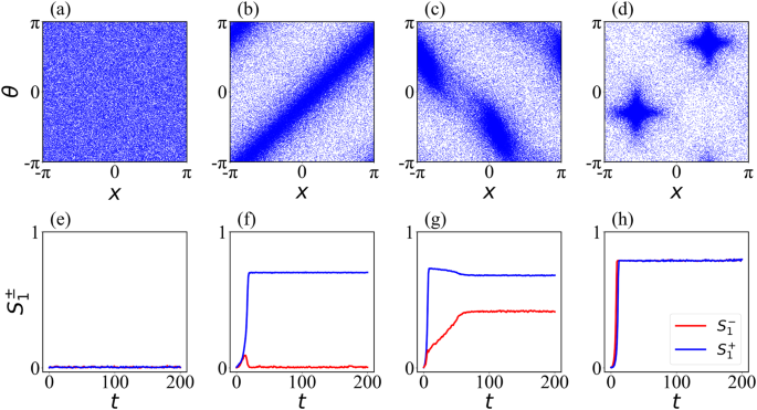

  

  a–d Scatter plots of all the four states in (x, θ) plane. e–h Time evolution of order parameters ${S}_{1}^{+}({S}_{1}^{-})$, depicted in blue (red). a and e represent the async state for a choice of coupling strengths (J₁, K₁, J₂, K₂) = (7, −1, 8, 9), b and f correspond to the phase wave state with (J₁, K₁, J₂, K₂) = (1, 6.5, 5, 9), c and g are associated with the mixed state for (J₁, K₁, J₂, K₂) = (9, 1.8, 6.5, 5.5), and the sync state is delineated in d, h for (J₁, K₁, J₂, K₂) = (9, 5, 6.5, 5.5). All the results are generated by integrating Eqs. (2a) and (2b) using Julia Tsit5 adaptive differential equation solver⁷⁶ with N = 10⁵ swarmalators whose intrinsic velocity and frequency have been drawn from the Lorentzian distribution with zero mean and half-width Δ_ω = Δ_v = 1.

• (ii) “Phase waves” or (S, 0) or (0, S) state [Fig. 1b, f]: In this state the swarmalators develop a band or phase wave, where the spatial positions x_i and phase angles θ_i are related as x_i ≈ ∓ θ_i, depending on whether it is (S, 0) or (0, S) state, respectively. In the (ξ, η) coordinate system, the swarmalators are partially locked in either ξ_i or η_i and drift in the other variable.

• (iii) The third state is referred to as the “Mixed state”, denoted by $({S}_{1}^{+},{S}_{1}^{-})=({S}^{{\prime} },{S}^{{\prime\prime} })$, where ${S}^{{\prime} }\,\ne \,{S}^{{\prime\prime} }\,\ne \,0$ (Fig. 1g). In this state, the swarmalators form a band where clusters of correlated swarmalators are observed to move together, as depicted in Fig. 1c.

• (iv) The fourth state is known as “Sync” state, denoted by (S, S), where S ≠ 0 [Fig. 1h]. In this state, the swarmalators are partially locked in both ξ_i and η_i. For most initial conditions, two clusters of locked swarmalators emerge spontaneously, as depicted in Fig. 1d. However, one can also observe a single cluster of locked swarmalators for some initial conditions.

Analysis

Next, in order to analyze all these four states, we employ the Ott-Antonsen (OA) ansatz⁶⁵ in the thermodynamic (N → ∞) limit and derive the expressions for order parameters in each state. In the N → ∞ limit, the collective states of the swarmalators can be defined by a continuous function ρ(v, ω, ξ, η, t) as,

$$\rho \equiv \frac{1}{N}\mathop{\sum }\limits_{j=1}^{N}\delta (v-{v}_{j})\delta (\omega -{\omega }_{j})\delta (\xi -{\xi }_{j})\delta (\eta -{\eta }_{j}),$$

(6)

where ρ(v, ω, ξ, η, t) is the probability to have a swarmalator at time t with intrinsic frequency ω, intrinsic velocity v, and coordinates η and ξ. Differentiating (6) with respect to t, one can obtain the continuity equation

$$\frac{\partial \rho }{\partial t}+\frac{\partial }{\partial \xi }(\dot{\xi }\rho )+\frac{\partial }{\partial \eta }(\dot{\eta }\rho )=0.$$

(7)

Given that our model is a higher-order Kuramoto model occurring on a torus, we are in pursuit of a “torodoidal” OA ansatz^34,65,69, which can be described as a multiplication of Poisson kernels,

$$\rho (v,\omega ,\xi ,\eta ,t)= \frac{1}{4{\pi }^{2}}{g}_{v}(v){g}_{\omega }(\omega )\left[1+\mathop{\sum }\limits_{p=1}^{\infty }{\alpha }^{p}{e}^{{{{{{{{\rm{i}}}}}}}}p\xi }+{{{{{{{\rm{c.c}}}}}}}}\right]\\ \times \left[1+\mathop{\sum }\limits_{q=1}^{\infty }{\beta }^{q}{e}^{{{{{{{{\rm{i}}}}}}}}q\eta }+{{{{{{{\rm{c.c}}}}}}}}\right],$$

(8)

where α(v, ω, t) and β(v, ω, t) are undetermined and need to be solved in a self-consistent manner, and “c.c” refers to the complex conjugate of its preceding terms. Now plugging the expression for ρ [given by Eq. (8)] into the continuity Eq. (7), we obtain that the Fourier modes α(v, ω, t) and β(v, ω, t) are subsequently constrained to adhere to the identical conditions for all harmonics p and q, which leads to the fulfillment of a coupled complex-valued differential equation as follows,

$$\dot{\alpha }=-{{{{{{{\rm{i}}}}}}}}(v+\omega )\alpha +\frac{1}{2}[{({H}_{1}^{+})}^{* }-{H}_{1}^{+}{\alpha }^{2}]+\frac{\alpha }{2}[{({H}_{2}^{-})}^{* }{\beta }^{* }-{H}_{2}^{-}\beta ],$$

(9a)

$$\dot{\beta }=-{{{{{{{\rm{i}}}}}}}}(v-\omega )\beta +\frac{1}{2}[{({H}_{2}^{+})}^{* }-{H}_{2}^{+}{\beta }^{2}]+\frac{\beta }{2}[{({H}_{1}^{-})}^{* }{\alpha }^{* }-{H}_{1}^{-}\alpha ],$$

(9b)

in the submanifold $\left\Vert \alpha \right\Vert =1=\left\Vert \beta \right\Vert$. Subsequently, the order parameters ${Z}_{m}^{\pm }$(m = 1, 2) become

$${Z}_{m}^{+}=\int\nolimits_{-\infty }^{\infty }dv\int\nolimits_{-\infty }^{\infty }d\omega {g}_{v}(v){g}_{\omega }(\omega ){\alpha }^{{* }^{m}}(v,\omega ,t),$$

(10a)

$${Z}_{m}^{-}=\int\nolimits_{-\infty }^{\infty }dv\int\nolimits_{-\infty }^{\infty }d\omega {g}_{v}(v){g}_{\omega }(\omega ){\beta }^{{* }^{m}}(v,\omega ,t).$$

(10b)

Equations (9a)–(10b) contain a set of self-consisting equations for the order parameters ${Z}_{m}^{\pm }$ in the N → ∞ limit.

Stability of the async state

In the async state, the order parameters ${Z}_{m}^{\pm }$ are zero. When ${Z}_{m}^{\pm }=0$, Eqs. (9a) and (9b) give the solutions ${\alpha }_{0}(v,\omega ,t)=\exp [-{{{{{{{\rm{i}}}}}}}}(v+\omega )t]$ and ${\beta }_{0}(v,\omega ,t)=\exp [-{{{{{{{\rm{i}}}}}}}}(v-\omega )t]$. Clearly, these solutions are self-consistent, as substituting them into the Eqs. (10a) and (10b) one can obtain ${Z}_{m}^{\pm }=\exp [-{{{{{{{\rm{i}}}}}}}}({\Delta }_{v}+{\Delta }_{\omega })t]$, which converges to zero in the t → ∞ limit.

Now, to investigate the stability of the async state, we introduce a small perturbation around the solutions α₀ and β₀ given by

$${\alpha }_{1}(v,\omega ,t)=\, \alpha (v,\omega ,t)-{\alpha }_{0}(v,\omega ,t),\\ {\beta }_{1}(v,\omega ,t)=\, \beta (v,\omega ,t)-{\beta }_{0}(v,\omega ,t).$$

(11)

This eventually gives the perturbed order parameters as

$${Z}_{11}^{+}=\, \int\nolimits_{-\infty }^{\infty }dv\int\nolimits_{-\infty }^{\infty }d\omega {g}_{v}(v){g}_{\omega }(\omega ){\alpha }_{1}^{* }(v,\omega ,t),\\ {Z}_{11}^{-}=\, \int\nolimits_{-\infty }^{\infty }dv\int\nolimits_{-\infty }^{\infty }d\omega {g}_{v}(v){g}_{\omega }(\omega ){\beta }_{1}^{* }(v,\omega ,t),$$

(12)

where we assume that $1\gg \left\Vert {\alpha }_{1}(v,\omega ,t)\right\Vert$, $\left\Vert {\beta }_{1}(v,\omega ,t)\right\Vert$ and $\left\Vert {Z}_{11}^{\pm }\right\Vert$. Substituting the expressions for α₁, β₁ and ${Z}_{11}^{\pm }$ into the Eqs. (9a) and (9b), and considering the terms up to first order, we obtain the following set of evolution equations

$${\dot{\alpha }}_{1}=\, -{{{{{{{\rm{i}}}}}}}}(v+\omega ){\alpha }_{1}+\frac{1}{2}[{J}_{1}^{+}{({Z}_{11}^{+})}^{* }-{J}_{1}^{+}{Z}_{11}^{+}{\alpha }_{0}^{2}]\\ \, +\frac{{\alpha }_{0}}{2{\beta }_{0}}[{J}_{1}^{-}{({Z}_{11}^{-})}^{* }-{J}_{1}^{-}{Z}_{11}^{-}{\beta }_{0}^{2}],$$

(13a)

$${\dot{\beta }}_{1}=\, -{{{{{{{\rm{i}}}}}}}}(v-\omega ){\beta }_{1}+\frac{1}{2}[{J}_{1}^{+}{({Z}_{11}^{-})}^{* }-{J}_{1}^{+}{Z}_{11}^{-}{\beta }_{0}^{2}]\\ \, +\frac{{\beta }_{0}}{2{\alpha }_{0}}[{J}_{1}^{-}{({Z}_{11}^{+})}^{* }-{J}_{1}^{-}{Z}_{11}^{+}{\alpha }_{0}^{2}].$$

(13b)

One can notice that the terms with α₀ and β₀ as a function of v and ω oscillate rapidly for t ≫ 1. These rapidly oscillating terms barely contribute when integrating over v and ω, and thus to approximate the integrals, we can neglect these small terms. Now, introducing a new variable τ = v + ω, α and β can be expressed as α(v, ω, t) = α(y, t), and β(v, ω, t) = β(y, t), respectively. Then, integrating the Eqs. (13a) and (13b) over v and ω, we eventually obtain

$$\frac{d{Z}_{11}^{+}}{dt}= \int\nolimits_{-\infty }^{\infty }dv\int\nolimits_{-\infty }^{\infty }d\omega {g}_{v}(v){g}_{\omega }(\omega )\frac{d{\alpha }_{1}^{* }}{dt} \\ = \int\nolimits_{-\infty }^{\infty }d\tau {{{{{{{\mathcal{G}}}}}}}}(\tau )\frac{d{\alpha }_{1}^{* }(\tau )}{dt}=\frac{{J}_{1}^{+}-2({\Delta }_{v}+{\Delta }_{\omega })}{2}{Z}_{11}^{+},$$

(14a)

$$\frac{d{Z}_{11}^{-}}{dt}= \int\nolimits_{-\infty }^{\infty }dv\int\nolimits_{-\infty }^{\infty }d\omega {g}_{v}(v){g}_{\omega }(\omega )\frac{d{\beta }_{1}^{* }}{dt} \\ = \int\nolimits_{-\infty }^{\infty }d\tau {{{{{{{\mathcal{G}}}}}}}}(\tau )\frac{d{\beta }_{1}^{* }(\tau )}{dt}=\frac{{J}_{1}^{+}-2({\Delta }_{v}+{\Delta }_{\omega })}{2}{Z}_{11}^{-},$$

(14b)

where

$${{{{{{{\mathcal{G}}}}}}}}(\tau )=\int\nolimits_{-\infty }^{\infty }dv\int\nolimits_{-\infty }^{\infty }d\omega {g}_{v}(v){g}_{\omega }(\omega )\delta [\tau -(v\pm \omega )]=\frac{{\Delta }_{v}+{\Delta }_{\omega }}{\pi [{\tau }^{2}+{({\Delta }_{v}+{\Delta }_{\omega })}^{2}]}.$$

(15)

To evaluate the integration, we use the fact that it has a residue τ = i(Δ_v + Δ_ω) in the upper half plane where ${\alpha }_{0}^{* }(\tau )$ and ${\beta }_{0}^{* }(\tau )$ are analytic. Now, the async state becomes stable when the perturbed order parameters ${Z}_{11}^{\pm }$ die out in time. Hence, from Eqs. (14a) and (14b), one can conclude that the async state becomes unstable when ${J}_{1}^{+}-2({\Delta }_{v}+{\Delta }_{\omega })\, > \,0$, or in other words the async state sustains its stability for ${J}_{1}^{+}-2({\Delta }_{v}+{\Delta }_{\omega })\, < \,0$. Therefore, the curve satisfying

$${J}_{1}^{+}=2({\Delta }_{v}+{\Delta }_{\omega }),$$

(16)

signifies the critical curve above which the async state loses its stability, and the swarmalators form a phase wave state. Equation (16) reveals that the transition from async state to phase wave state depends solely on the pairwise interactions by means of the pairwise coupling strengths (J₁, K₁).

Analysis of phase wave state

In the phase wave state, swarmalators develop a phase wave or band with x_i = ∓ θ_i for (S, 0) and (0, S) states, respectively. Therefore, we seek a solution to Eqs. (9a)–(10b) that satisfies $\dot{\alpha }=0$, $\dot{\beta }\,\ne \,0$, ${Z}_{m}^{+}\,\ne \,0$, and ${Z}_{m}^{-}=0$, (m = 1, 2). Substituting these relations into the Eqs. (9a) and (9b), we have

$$0=-{{{{{{{\rm{i}}}}}}}}(v+\omega )\alpha +\frac{1}{2}[{({H}_{1}^{+})}^{* }-{H}_{1}^{+}{\alpha }^{2}],$$

(17a)

$$\dot{\beta }=-{{{{{{{\rm{i}}}}}}}}(v-\omega )\beta +\frac{\beta }{2\alpha }[{({H}_{1}^{-})}^{* }-{H}_{1}^{-}{\alpha }^{2}].$$

(17b)

Notice that α(v, ω, t) depends on v + ω, which is distributed according to a Lorentzian distribution with spread Δ_v + Δ_ω. This allows us to evaluate the integral for the order parameter ${Z}_{m}^{+}$ explicitly as ${Z}_{1}^{+}={\alpha }^{* }(i{\Delta }_{v}+i{\Delta }_{\omega },t)$ using the Cauchy’s residue theorem by closing the contour to an infinite-radius semicircle in the upper half-plane. Similarly, we can obtain ${Z}_{2}^{+}={\alpha }^{{* }^{2}}(i{\Delta }_{v}+i{\Delta }_{\omega },t)={({Z}_{1}^{+})}^{2}$. Substituting the relation between ${Z}_{1}^{+}$ and ${Z}_{2}^{+}$ into the Eqs. (17a) and (17b), and assuming ${\psi }_{1}^{+}=0$, we obtain the expressions for α and β as follows,

$$\alpha (v,\omega )={{{{{{{\mathcal{F}}}}}}}}\left(\frac{v+\omega }{{S}_{1}^{+}({J}_{1}^{+}+{({S}_{1}^{+})}^{2}{J}_{2}^{+})}\right),$$

(18)

and

$$\beta (v,\omega ,t)={e}^{(-rt)},$$

(19)

where we introduce a function ${{{{{{{\mathcal{F}}}}}}}}$ as

$${{{{{{{\mathcal{F}}}}}}}}(y)=-{{{{{{{\rm{i}}}}}}}}y+\sqrt{1-{y}^{2}},$$

(20)

and the term r is given by,

$$r= \, {{{{{{{\rm{i}}}}}}}}(v-\omega )-\frac{1}{2\alpha }[{({H}_{1}^{-})}^{* }-{H}_{1}^{-}{\alpha }^{2}]={{{{{{{\rm{i}}}}}}}}\left[\frac{{J}_{1}{K}_{1}}{{J}_{1}^{+}+{({S}_{1}^{+})}^{2}{J}_{2}^{+}}\left(\frac{v}{{J}_{1}}-\frac{\omega }{{K}_{1}}\right)\right. \\ + \left.\frac{{({S}_{1}^{+})}^{2}{J}_{2}{K}_{2}}{{J}_{1}^{+}+{({S}_{1}^{+})}^{2}{J}_{2}^{+}}\left(\frac{v}{{J}_{2}}-\frac{\omega }{{K}_{2}}\right)\right].$$

(21)

Equation (19) results in ${Z}_{m}^{-}=0$, as anticipated. On the other hand, Eq. (18) implies that

$${S}_{1}^{+}={{{{{{{{\mathcal{F}}}}}}}}}^{* }\left(\frac{{{{{{{{\rm{i}}}}}}}}{\Delta }_{v}+{{{{{{{\rm{i}}}}}}}}{\Delta }_{\omega }}{{S}_{1}^{+}({J}_{1}^{+}+{({S}_{1}^{+})}^{2}{J}_{2}^{+})}\right).$$

(22)

Solving Eq. (22) for ${S}_{1}^{+}$ gives the expression of ${S}_{1}^{+}$ as

$${S}_{1}^{+}=\sqrt{\frac{{J}_{2}^{+}-{J}_{1}^{+}\pm \sqrt{{\left({J}_{1}^{+}+{J}_{2}^{+}\right)}^{2}-8{J}_{2}^{+}\tilde{\Delta }}}{2{J}_{2}^{+}}},$$

(23)

where $\tilde{\Delta }={\Delta }_{v}+{\Delta }_{\omega }$. The plus and minus sign inside the square root corresponds to the stable and unstable solutions if they exist. Equation (23) suggests the presence of a bistable region upon the selection of coupling strengths. In this scenario, a particular combination of coupling values leads to the coexistence of asynchronous and phase wave states depending on the initial conditions chosen. Saying differently, with varying coupling strengths, there exist two different transition scenarios: one corresponds to the transition from the async state to the phase wave state, referred to as forward transition, and the other is backward transition, which is associated with the transition from phase wave state to async state. For the forward transition case, ${S}_{1}^{+}$ bifurcates from 0 (i.e., async state) at

$${J}_{1,f}^{+}=2\tilde{\Delta }=2({\Delta }_{v}+{\Delta }_{\omega }),$$

(24)

which is consistent with Eq. (16), where forward transition from async state to phase wave state emerges and only the stable branch of ${S}_{1}^{+}$ exists. This once again guarantees that the transition from async state to phase wave state is solely dependent on the pairwise coupling strengths. On the other hand, in the case of backward transition, both the stable and unstable branches coexist for a region of parameter values called the hysteresis region. But as soon as the backward critical coupling condition ${J}_{1}^{+}={J}_{1,b}^{+}$ is reached, both the stable and unstable branches clash and destroy each other. As a result, the stability of the phase wave is completely shattered, and ${S}_{1}^{+}=0$ is the sole viable solution. From Eq. (23), we obtain that both the stable and unstable branches of ${S}_{1}^{+}$ exist if the following coupling condition satisfies,

$${J}_{1,b}^{+}=2\sqrt{2{J}_{2}^{+}\tilde{\Delta }}-{J}_{2}^{+}.$$

(25)

Equation (25) thus corresponds to the critical curve for the backward transition.

To illustrate this, we numerically integrate the Eqs. (2a) and (2b) with N = 10⁵ swarmalators for the calculation of ${S}_{1}^{\pm }$. In Fig. 2a we plot the variation of order parameter ${S}_{1}^{\pm }$ as a function of pairwise coupling strength K₁. K₁ is first increased adiabatically from K₁ = 0 to an adequately large value and then decreased back with the other couplings fixed at J₁ = 1, J₂ = 5, and K₂ = 9. The results reveal that ${S}_{1}^{-}$ remains zero all the time, while an abrupt transition from ${S}_{1}^{+}\,\approx \,0$ to ${S}_{1}^{+}\,\approx \, 0.7$ occurs at K₁ = 7 [obtained from Eq. (24)] as the coupling strength K₁ is increased. Another abrupt transition from ${S}_{1}^{+}\,\approx \,1$ to ${S}_{1}^{+}\,\approx \,0$ occurs at K₁ = 6 [obtained from Eq. (25)] as K₁ is decreased starting from the phase wave state. Therefore, the system supports bistability behavior (where both phase wave and async states are stable) for K₁ ∈ [6, 7]. This is further substantiated by our theoretical predictions regarding the order parameters (illustrated using continuous and dashed magenta lines for the stable and unstable branches, respectively), demonstrating a commendable concurrence with the numerical findings (represented by solid circles). To emphasize the bistability nature, in Fig. 3 we demonstrate the async (Fig. 3a, b) and phase wave (Fig. 3c, d) states, respectively, for K₁ = 6.5 while keeping the other couplings fixed at specific values as earlier.

Fig. 2: Abrupt transition from the async state to the phase wave state.

a Order parameter ${S}_{1}^{\pm }$ as a function of pairwise coupling strength K₁ for J₁ = 1 and fixed three-body coupling strengths J₂ = 5, K₂ = 9. Solid and dashed magenta curves represent the stable and unstable solutions given by Eq. (23), respectively. The dashed vertical lines correspond to the critical couplings for forward (in red) and backward (in black) transitions obtained from Eqs. (24) and (25), respectively. Solid circles depict the result obtained from the direct simulation of Eqs. (2a) and (2b) for N = 10⁵ oscillators with half widths of the Lorentzian distribution Δ_v = Δ_ω = 1. The results reveal an abrupt transition from async (I) state to phase wave (III) state, which results in a bistable domain (II) where both the referred states are stable. b The comprehensive stability diagram illustrating the states of async (I), phase wave (III) and bistability (II) as a function of pairwise coupling ${J}_{1}^{+}=\frac{{J}_{1}+{K}_{1}}{2}$ and higher-order coupling ${J}_{2}^{+}=\frac{{J}_{2}+{K}_{2}}{2}$. Two distinct types of bifurcations, saddle-node and pitchfork, are represented by blue and red curves, respectively. These two curves intersect each other at $({J}_{1}^{+},{J}_{2}^{+})=(4,4)$. When ${J}_{2}^{+} < 4$, the pitchfork bifurcation is deemed supercritical, whereas when ${J}_{2}^{+}\, > \,4$, the pitchfork bifurcation becomes subcritical.

Fig. 3: Bistablilty between async and phase wave state.

Scatter plot for async (0, 0) and phase wave (S, 0) states at K₁ = 6.5, J₁ = 1, J₂ = 5, and K₂ = 9 [drawn from the region (II) in Fig. 2a] is depicted in panels a-b and c-d, respectively. The order parameter ${S}_{1}^{+}({S}_{1}^{-})$ is indicated by the black (magenta) circle in a and c, where the values of ${S}_{1}^{+}$ and ${S}_{1}^{-}$ are represented by the length of the line joining the center with the respective circles. Clearly, in a, both the values of order parameters are almost zero, indicating the async (0, 0) state, while in c, the value of ${S}_{1}^{+}$ is non-zero and ${S}_{1}^{-}$ is zero, characterizing the phase wave (S, 0) state. In panels b and d, the corresponding scatter plots in the (x, θ) plane are displayed. Swarmalators are uniformly distributed in both phase and space, characterizing the async state (in b), whereas in panel d, swarmalators display a correlation between phase and space and thus correspond to the phase wave state.

The outcomes given above highlight a significant finding that the introduction of higher-order interactions can cause a sudden transition from the async state to phase wave state and vice-versa, which was not the case with only pairwise interactions among the swarmalators³⁴. Thereafter, to better understand the effect of higher-order interactions in promoting bistability behavior, we plot the complete stability profile for the system in Fig. 2b. It shows that for adequately small values of higher-order coupling $({J}_{2}^{+} \, < \, 4)$, the transition from async state (I) to phase wave state (III) is continuous and takes place through a supercritical pitchfork bifurcation at ${J}_{1}^{+}=4$. However, for larger values of higher-order coupling $({J}_{2}^{+} \, > \, 4)$, the pitchfork bifurcation at ${J}_{1}^{+}=4$ becomes subcritical and a saddle-node bifurcation emerges at a lower value of ${J}_{1}^{+}$, given by Eq. (25) (depicted in blue). These two bifurcations correspond to the sudden transition observed in Fig. 2a, and the region bounded by them refers to the region of bistability (II) between async and phase wave state. Figure 2b also reveals an interesting observation that for relatively larger values of higher-order coupling $({J}_{2}^{+}\ge 16)$, the region of bistability stretches into the negative region ${J}_{1}^{+}\, < \,0$, demonstrating the fact that higher-order interactions can stabilize the phase wave state even when the pairwise interactions are repulsive.

Analysis of sync state

In the sync state we have $({S}_{1}^{+},{S}_{1}^{-})=(S,S)$, with S ≠ 0. Therefore, we seek solutions to the Eqs. (9a)–(10b) such that ${Z}_{m}^{\pm }\, \ne \, 0\,$(m = 1, 2). We will here analyze the sync state in two cases: one when J₁ = K₁, J₂ = K₂ and the other for an arbitrary combination of pairwise and higher-order couplings, i.e., for a generic case.

Specific case: J₁ = K₁ and J₂ = K₂

In this case, the coupled complex-valued differential Eqs. (9a) and (9b) become decoupled as follows

$$\dot{\alpha }=-{{{{{{{\rm{i}}}}}}}}(v+\omega )\alpha +\frac{1}{2}[{({H}_{1}^{+})}^{* }-{H}_{1}^{+}{\alpha }^{2}],$$

(26a)

$$\dot{\beta }=-{{{{{{{\rm{i}}}}}}}}(v-\omega )\beta +\frac{1}{2}[{({H}_{2}^{+})}^{* }-{H}_{2}^{+}{\beta }^{2}],$$

(26b)

and consequently the phases ξ and η develop independently analogous to typical higher-order Kuramoto model⁴⁵. From Eqs. (26a) and (26b) one can observe that the functions α and β are dependent on (v + ω) and (v − ω), respectively, which are distributed in accordance with a Lorentzian distribution characterized by a spread of (Δ_v + Δ_ω). This allows us to evaluate the integrals for the order parameters ${Z}_{1}^{\pm }$ explicitly as ${Z}_{1}^{+}={\alpha }^{* }(i{\Delta }_{v}+i{\Delta }_{\omega },t)$ and ${Z}_{1}^{-}={\beta }^{* }(i{\Delta }_{v}+i{\Delta }_{\omega },t)$ using the residue theorem. Similarly the other order parameters ${Z}_{m}^{\pm }$ can be obtained explicitly as ${Z}_{2}^{+}={\alpha }^{{* }^{2}}(i{\Delta }_{v}+i{\Delta }_{\omega },t)={({Z}_{1}^{+})}^{2}$ and ${Z}_{2}^{-}={\beta }^{{* }^{2}}(i{\Delta }_{v}+i{\Delta }_{\omega },t)={({Z}_{1}^{+})}^{2}$. Substituting these into Eqs. (26a) and (26b) give

$${\dot{{Z}_{1}}}^{\pm }= \, -({\Delta }_{v}+{\Delta }_{\omega }){Z}_{1}^{\pm }+\frac{1}{2}\left[\left\{{K}_{1}{Z}_{1}^{\pm }+{K}_{2}{({Z}_{1}^{\pm })}^{2}{({Z}_{1}^{\pm })}^{* }\right\}\right.\\ -\left.\left\{{K}_{1}{({Z}_{1}^{\pm })}^{* }+{K}_{2}{({Z}_{1}^{\pm })}^{{* }^{2}}({Z}_{1}^{\pm })\right\}{({Z}_{1}^{\pm })}^{2}\right].$$

(27)

As anticipated, the above equations are similar to those of the typical higher-order Kuramoto model⁴⁵ with Lorentzian natural frequency having half width (Δ_v + Δ_ω). Assuming ${\psi }_{1}^{\pm }$ to be zero, we can obtain the steady state solution for the order parameters corresponding to the sync state ${S}_{1}^{+}={S}_{1}^{-}=S$ as

$$S=\sqrt{\frac{{K}_{2}-{K}_{1}\pm \sqrt{{\left({K}_{1}+{K}_{2}\right)}^{2}-8{K}_{2}\tilde{\Delta }}}{2{K}_{2}}},$$

(28)

where plus and minus signs correspond to the stable and unstable solutions if they exist. Equation (28) resembles the solution for phase wave state, given by Eq. (23) when J₁ = K₁ and J₂ = K₂. This suggests that the transition from async (0, 0) state to sync (S, S) state can emerge without experiencing an intermediate phase wave (S, 0) or (0, S) state and the forward transition occurs at the same critical coupling given by

$${J}_{1}={K}_{1}=2({\Delta }_{v}+{\Delta }_{\omega }).$$

(29)

To illustrate this, in Fig. 4a we plot the order parameters ${S}_{1}^{\pm }$ as a function of K₁ with fixed higher-order coupling strengths J₂ = K₂ = 9. The solid and dashed magenta curves depict the analytical predictions provided by Eq. (28) for the stable and unstable branches, respectively, which are in good agreement with the outcomes obtained through direct simulation (represented by circles). With increasing K₁, we observe a sudden transition from ${S}_{1}^{\pm }\,\approx \,0$ (async state) to ${S}_{1}^{\pm }\approx 1$ (sync state) at K₁ = 4 [given by Eq. (29)]. Another abrupt transition from ${S}_{1}^{\pm }\approx \,1$ to ${S}_{1}^{\pm }\approx \,0$ emerges at K₁ = 3 [obtained from Eq. (25) for J₁ = K₁ and J₂ = K₂] as K₁ is decreased adiabatically starting from the sync state. Thus, within the domain bounded by these two sudden transitions, the system exhibits a bistable nature where both the sync and async states are achievable for any specific value of coupling strength. To highlight the presence of bistability, we showcase the two distinct states for K₁ = 3.5 in Fig. 5: asynchronous state (Fig. 5a, b) and synchronous state (Fig. 5c, d). Besides, in Fig. 4b we plot the stability diagram for the system, which shows that beyond K₂ = 4, a bistable dynamics emerges in the system due to the interplay between saddle-node and subcritical pitchfork bifurcations, and the associated region of bistability (II) is bounded by the curves of these bifurcations. On the other hand, for K₂ < 4, a continuous transition from async state (I) to sync state (III) occurs at K₁ = 4 through a supercritical pitchfork bifurcation. The stretch of the bistability region (II) in the regime K₁ < 0 reveals the fact that for sufficiently larger higher-order coupling strengths, the system can achieve a stable sync state even when the pairwise interactions are repulsive (i.e., K₁ = J₁ < 0).

Fig. 4: Abrupt transition from async to sync state.

In a, the behavior of the order parameter ${S}_{1}^{\pm }$ is presented in relation to the pairwise coupling strength K₁. With a fixed setting of J₁ = K₁ and constant three-body coupling strengths J₂ = K₂ = 9, both stable and unstable solutions (obtained from Eq. (28)) are showcased through solid and dashed magenta curves, respectively. The dashed vertical lines correspond to critical coupling values for forward (red) and backward (black) transitions. These values are derived from Eqs. (29) and (25), with J₁ = K₁, J₂ = K₂. The outcome obtained from direct simulations of Eqs. (2a) and (2b) is depicted in solid circles for N = 10⁵ swarmalators with Lorentzian distribution half-widths Δ_ω = Δ_v = 1. The findings distinctly reveal an abrupt transition from the async (I) state to the sync (III) state, establishing a bistable domain (II) where both states are stable. Moving to b, a comprehensive stability diagram is presented, illustrating the states of async (I), phase wave (III), and bistability (II) as functions of pairwise coupling K₁ and higher-order coupling K₂. The diagram encompasses two distinct types of bifurcations: the blue curve representing a saddle-node bifurcation and the red curve depicting a pitchfork bifurcation. Notably, these curves intersect at (K₁, K₂) = (4, 4). When K₂ < 4, the pitchfork bifurcation takes a supercritical nature, whereas, for K₂ > 4, the pitchfork bifurcation becomes subcritical.

Fig. 5: Bistablilty between async and sync state.

Scatter plot for async (0, 0) and sync (S, S) states at K₁ = J₁ = 3.5, and K₂ = J₂ = 9 [drawn from the region (II) in Fig. 4a] is depicted in panels a-b and c-d, respectively. The order parameter ${S}_{1}^{+}({S}_{1}^{-})$ is indicated by the black (magenta) circle in a and c, where the values of ${S}_{1}^{+}$ and ${S}_{1}^{-}$ are represented by the length of the line joining the center with the respective circles. Clearly, in panel a, the values of both order parameters are almost zero, indicating the async (0, 0) state, while in c, both the order parameters take non-zero equal value, characterizing the sync (S, S) state. In panels b and d, the corresponding scatter plots in the (x, θ) plane are displayed. Swarmalators are uniformly distributed in both phase and space, characterizing the async state (in panel b), whereas in d, swarmalators are locked in both phase and space and thus correspond to the sync state.

General case: J₁ ≠ K₁ and J₂ ≠ K₂

In contrast to the earlier scenario, in this case, the coupled complex-valued differential Eqs (9a) and (9b) cannot be separated from each other. As a result, it’s not possible to directly express the order parameters ${Z}_{1}^{\pm }$ in terms of α and β, respectively. Therefore, we look for a solution of Eqs. (9a) and (9b) that satisfy $\dot{\alpha }=0,\dot{\beta }=0,{Z}_{m}^{\pm }\,\ne \,0$. Assuming ${\psi }_{m}^{\pm }=0$, we find

$$\alpha (v,\omega )={{{{{{{\mathcal{F}}}}}}}}\left[\frac{{A}_{1}+{A}_{2}{({S}_{1}^{-})}^{2}}{{S}_{1}^{+}\{C({S}_{1}^{{+}^{2}}+{S}_{1}^{{-}^{2}})+2(D+E{S}_{1}^{{+}^{2}}{S}_{1}^{{-}^{2}})\}}\right],$$

(30a)

$$\beta (v,\omega )={{{{{{{\mathcal{F}}}}}}}}\left[\frac{{B}_{1}+{B}_{2}{({S}_{1}^{+})}^{2}}{{S}_{1}^{-}\{C({S}_{1}^{{+}^{2}}+{S}_{1}^{{-}^{2}})+2(D+E{S}_{1}^{{+}^{2}}{S}_{1}^{{-}^{2}})\}}\right],$$

(30b)

where

$${A}_{1,2}= \,2(v{K}_{1,2}+\omega {J}_{1,2}),\ {B}_{1,2}=2(v{K}_{1,2}-\omega {J}_{1,2}),\\ C= \,{J}_{1}{K}_{2}+{J}_{2}{K}_{1},\ D={J}_{1}{K}_{1},\ E={J}_{2}{K}_{2}.$$

(31)

Now, we solve the integrals for the order parameters given by Eqs. (10a) and (10b) using residue theorem. Further, considering the fact that in the sync state ${S}_{1}^{+}={S}_{1}^{-}=S$, we obtain

$$S={{{{{{{{\mathcal{F}}}}}}}}}^{* }\left[\frac{{\Delta }_{1}+{\Delta }_{2}{S}^{2}}{S\{2C{S}^{2}+2(D+E{S}^{4})\}}\right],$$

(32)

where Δ_1,2 = 2(Δ_vK_1,2 + Δ_ωJ_1,2). Equation (32) eventually provides the expression for the order parameter, which can be acquired by solving the following equation for S

$$E{y}^{3}+(C-E){y}^{2}+({\Delta }_{2}-C+D)y+({\Delta }_{1}-D)=0,$$

(33)

where y = S². From Eq. (33), it is clear that S bifurcates from zero at Δ₁ = D, i.e.,

$$2\left(\frac{{\Delta }_{v}}{{J}_{1}}+\frac{{\Delta }_{v}}{{K}_{1}}\right)=1.$$

(34)

Notice that for J₁ = K₁, the condition (34) coincides with the critical coupling condition (29) and thus once again guarantees that the sync state can bifurcate directly from the async state without passing through any intermediate state [Fig. 4]. However, in general circumstances (i.e., J₁ ≠ K₁, J₂ ≠ K₂), the transition from async state to sync state is not direct but occurs by passing through intermediate states, namely phase wave state and mixed state. To describe this, in Fig. 6 we plot the order parameters ${S}_{1}^{\pm }$ for varying K₁ while keeping the other couplings fixed at nominal values J₁ = 9, J₂ = 6.5, and K₂ = 5.5. The solid magenta and blue lines correspond to the analytical predictions of stable solutions of phase and sync states obtained from Eqs. (23) and (33), respectively, which are in favorable alignment with the results obtained through direct simulation (shown in solid and void markers) for the finite-size system. As observed, with increasing K₁, the system passes from the async state (I) to the sync state (V) through the intermediate phase wave state (III) and mixed state (IV). Here, the evolution of the order parameters $({S}_{1}^{+},{S}_{1}^{-})$ shows that with increasing K₁, the system passes from (0, 0) (i.e., async) state to (S, 0) (i.e., phase wave) state through an abrupt transition, resulting into an interval of bistability (II) where both the async and phase wave states are stable. On the other hand, the system goes through a continuous transition from (S, 0) (i.e., phase wave) state to (S, S) (i.e., sync) state, resulting in the intermediate mixed state $({S}^{{\prime} },{S}^{{\prime\prime} })$ where ${S}^{{\prime} }\, > \,{S}^{{\prime\prime} }$.

Fig. 6: Transition from async to sync state through intermediate mixed state.

Order parameter ${S}_{1}^{\pm }$ as a function of pairwise coupling strength K₁ for J₁ = 9 and fixed three-body coupling strengths J₂ = 6.5, K₂ = 5.5. Solid magenta and blue curves represent the stable solutions for phase wave and sync states, given by Eqs. (23) and (33), respectively. Solid circles depict the result obtained from the direct simulation of Eqs. (2a) and (2b) for N = 10⁵ oscillators with half widths of the Lorentzian distribution Δ_v = Δ_ω = 1. An abrupt transition from the async (I) to phase wave (III) state is observed, which creates a domain of bistability (II), where both the states are stable. On the other hand, from the phase wave state (III) to sync state (V), a smooth (continuous) transition occurs, resulting in the shaded region (IV), which corresponds to $({S}^{{\prime} },{S}^{{\prime\prime} })$ state, with ${S}^{{\prime} }\, > \,{S}^{{\prime\prime} }$, and called as mixed state.

Mixed state

In the mixed state we have $({S}_{1}^{+},{S}_{1}^{-})=({S}^{{\prime} },{S}^{{\prime\prime} })$, with ${S}^{{\prime} }\,\ne \,{S}^{{\prime\prime} }$. This state resides as an intermediary between the phase wave and sync states and bifurcates from the (S, 0), or (0, S) state when ${S}^{{\prime} }\, > \,{S}^{{\prime\prime} }$ or ${S}^{{\prime\prime} }\, > \,{S}^{{\prime} }$, through a continuous transition to the (S, S) state. In Fig. 6, the shaded black region (IV) depicts the interval of K₁ (keeping the other coupling fixed at a nominal value) for which the system passes through the mixed state. Unfortunately, we are unable to find the analytical boundaries in terms of the coupling strengths for the mixed state, and thus obtain the domain of mixed state through the numerical investigations by evaluating the order parameters ${S}_{1}^{\pm }$ with ${S}_{1}^{+} \, > \, {S}_{1}^{-}$. The distinctive characteristic of the mixed state lies in the fact that while both ${S}^{{\prime} }$ and S^″ remain time-independent, the functions α and β exhibit time dependency³⁴. This contrasts with the time-independent Eqs. (18) and (30) associated with the phase wave and sync states, respectively.

Abrupt transition from phase wave state to sync state

As discussed above, in general, with increasing coupling strengths, a continuous transition from the phase wave state to the sync state emerges in the system through an intermediate mixed state. This smooth transition phenomenon is consistent with previously acquired results for only pairwise interactions between the swarmalators³⁴. When the higher-order coupling strengths are relatively small, a comparable transition phenomenon is still evident in our present system with higher-order interactions [Fig. 6]. Conversely, when sufficiently significant higher-order couplings come into play, a critical observation comes to light. In this scenario, the influence of higher-order interactions leads to an abrupt and noteworthy transition from the (S, 0)/(0, S) state to the (S, S) state, bypassing the intermediate mixed state. To illustrate this, in Fig. 7 we plot the order parameters $({S}_{1}^{+},{S}_{1}^{-})$ as a function of K₁ for adequately large higher-order couplings J₂ = 8 and K₂ = 9, keeping J₁ fixed at J₁ = 7. The solid magenta and blue lines represent the analytically predicted stable solutions for the phase and synchronized states, respectively, derived from Eqs. (23) and (33). Impressively, these analytical predictions closely match the outcomes obtained through direct simulations on the finite size system, depicted by the solid and void markers. As K₁ is being first adiabatically increased to a large value and then decreased, we observe two different abrupt transitions, resulting in two distinct bistable domains. The first one corresponds to a sudden transition from the (0, 0) state (I) to the (S, 0) state (III), inducing a region of bistability (II), where both the async and phase wave states are stable (shaded gray region). This bistable phenomenon has already been addressed in the context of analyzing the phase wave state. The second one is associated with an abrupt transition from (S, 0) state (III) to (S, S) state (V), giving rise to a bistable domain (IV), where both stable phase wave and sync state can emerge (shaded red region). To elucidate this bistability nature, in Fig. 8, we demonstrate the two distinct states: phase wave state (Fig. 8a, b) and sync state (Fig. 8c, d) for fixed K₁ = 1.5, drawn from the region of bistability (IV).

Fig. 7: Abrupt transitions from async to phase wave state, and phase wave to sync state.

Order parameter ${S}_{1}^{\pm }$ as a function of pairwise coupling strength K₁ for J₁ = 7 and fixed three-body coupling strengths J₂ = 8, K₂ = 9. Solid magenta and blue curves represent the stable solutions for phase wave and sync states, given by Eqs. (23) and (33), respectively. Solid circles depict the result obtained from the direct simulation of Eqs. (2a) and (2b) for N = 10⁵ oscillators with half widths of the Lorentzian distribution Δ_v = Δ_ω = 1. Two distinct abrupt transitions are revealed. First, an abrupt transition from the async (I) to phase wave (III) state is observed, which creates a domain of bistability (II), where both the async and phase wave states are stable. Second, from the phase wave state (III) to sync state (V), generating a bistable domain (IV), where both the phase wave and sync states are stable.

Fig. 8: Bistablilty between phase wave and sync state.

Scatter plot for phase wave (S, 0) and sync (S, S) states at K₁ = 1.5, J₁ = 7, K₂ = 9, and J₂ = 8 [drawn from the region (IV) in Fig. 7] is depicted in panels a-b and c-d, respectively. The order parameter ${S}_{1}^{+}({S}_{1}^{-})$ is indicated by the black (magenta) circle in a and c, where the values of ${S}_{1}^{+}$ and ${S}_{1}^{-}$ are represented by the length of the line joining the center with the respective circles. Clearly, in panel a, the value of ${S}_{1}^{+}$ is non-zero, and ${S}_{1}^{-}$ is zero, representing the phase wave (S, 0) state, while in c, both the order parameters take non-zero equal value, characterizing the sync (S, S) state. In panels b and d, the corresponding scatter plots in the (x, θ) plane are displayed. Swarmalators display a correlation between phase and space in panel b, characterizing the async state, whereas, in d, swarmalators are locked in both phase and space and thus correspond to the sync state.

Conclusion

Summing up, here we have introduced an analytically tractable model of swarmalators that incorporates both pairwise and higher-order interactions (specifically three-body interactions), embedded in a simplicial complex at the microscopic level. This proposed model exhibits a high degree of complexity with four distinct collective states, namely async, phase wave, mixed, and sync states. The higher-order interactions introduce supplementary layers of nonlinearity into the behavior of the macroscopic system dynamics. As a result, a few pivotal phenomena emerge that remain absent when interactions between the swarmalators are confined to only pairwise connections and lack the influence of higher-order interactions. We observe that the inclusion of higher-order interactions leads to abrupt transitions from the async state to either the phase wave state or the sync state, depending on the specific coupling strength configurations. Our observations also reveal that when the higher-order interactions are sufficiently strong, phase wave and sync state can emerge and persist, even in scenarios where pairwise couplings are repulsive. This implies that despite the potential decay of specific coupling types, the existence of alternative forms of coupling can play a pivotal role in upholding the regimes of bistability between async and phase wave (sync) states. Furthermore, our findings extend to the discovery that substantial higher-order couplings can facilitate a direct emergence of the sync state from the phase wave state without passing through the mixed state. This distinct behavior stands in contrast to situations involving solely pairwise interactions, where the synchronized state bifurcates from the phase wave state through the intermediate mixed state. Our obtained collective states, such as phase wave and sync state, adeptly resemble the collective dynamics observed in active matter and real-world swarmalators, exemplified by collective behaviors observed in vinegar eels⁵, group of sperm⁷⁰, and forced colloids including Janus particles^6,7,71. Additionally, our observed phase transitions resemble the disordered to order transition in real-world swarmalators systems, including biological microswimmers such as ensemble of sperm^70,72 and system of Janus particles⁷³.

Thus, our theoretical study makes a substantial contribution to understanding the influence of higher-order interactions on shaping the collective dynamics of swarmalators, although numerous avenues for further exploration remain open. In this context, we specifically focus on higher-order interactions up to the third order, employing an all-to-all coupling arrangement. Consequently, investigating interactions beyond the three-body and exploring localized coupling configurations becomes a particularly intriguing prospect for future research. It is also worth noting that our current investigation is limited to analyzing the effect of higher-order interactions solely within a 1D swarmalator model on a ring. As such, an equally captivating avenue for future exploration lies in examining how higher-order interactions impact the collective behavior within 2D and other higher-dimensional swarmalator systems. Lastly, we believe our results can be substantiated through empirical testing within the dynamic environment of robotic swarms or within the confines of circularly confined colloids^3,74 by incorporating beyond pairwise interactions.

References

Ota, K., Aihara, I. & Aoyagi, T. Interaction mechanisms quantified from dynamical features of frog choruses. R. Soc. Open Sci. 7, 191693 (2020).
Hrabec, A. et al. Velocity enhancement by synchronization of magnetic domain walls. Phys. Rev. Lett. 120, 227204 (2018).
Barciś, A. & Bettstetter, C. Sandsbots: Robots that sync and swarm. IEEE Access 8, 218752–218764 (2020).
Belovs, M., Livanovičs, R. & Cēbers, A. Synchronized rotation in swarms of magnetotactic bacteria. Phys. Rev. E 96, 042408 (2017).
Peshkov, A., McGaffigan, S. & Quillen, A. C. Synchronized oscillations in swarms of nematode turbatrix aceti. Soft Matter 18, 1174–1182 (2022).
Zhang, B., Sokolov, A. & Snezhko, A. Reconfigurable emergent patterns in active chiral fluids. Nat. Commun. 11, 4401 (2020).
Yan, J., Bloom, M., Bae, S. C., Luijten, E. & Granick, S. Linking synchronization to self-assembly using magnetic janus colloids. Nature 491, 578–581 (2012).
Pikovsky, A., Rosenblum, M., Kurths, J. & Synchronization, A. A universal concept in nonlinear sciences. Self 2, 3 (2001).
Boccaletti, S., Pecora, L. M. & Pelaez, A. Unifying framework for synchronization of coupled dynamical systems. Phys. Rev. E 63, 066219 (2001).
Sumpter, D. J.Collective animal behavior (Princeton University Press, 2010).
Bialek, W. et al. Statistical mechanics for natural flocks of birds. Proc. Natl Acad. Sci. 109, 4786–4791 (2012).
Reynolds, C. W. Flocks, herds and schools: A distributed behavioral model. In Proceedings of the 14th annual conference on Computer graphics and interactive techniques, 25–34 (ACM, 1987).
Vicsek, T., Czirók, A., Ben-Jacob, E., Cohen, I. & Shochet, O. Novel type of phase transition in a system of self-driven particles. Phys. Rev. Lett. 75, 1226 (1995).
Stilwell, D. J., Bollt, E. M. & Roberson, D. G. Sufficient conditions for fast switching synchronization in time-varying network topologies. SIAM J. Appl. Dyn. Syst. 5, 140–156 (2006).
Frasca, M., Buscarino, A., Rizzo, A., Fortuna, L. & Boccaletti, S. Synchronization of moving chaotic agents. Phys. Rev. Lett. 100, 044102 (2008).
Uriu, K., Ares, S., Oates, A. C. & Morelli, L. G. Dynamics of mobile coupled phase oscillators. Phys. Rev. E 87, 032911 (2013).
Tanaka, D. General chemotactic model of oscillators. Phys. Rev. Lett. 99, 134103 (2007).
Iwasa, M. & Tanaka, D. Dimensionality of clusters in a swarm oscillator model. Phys. Rev. E 81, 066214 (2010).
Iwasa, M., Iida, K. & Tanaka, D. Hierarchical cluster structures in a one-dimensional swarm oscillator model. Phys. Rev. E 81, 046220 (2010).
O’Keeffe, K. P., Hong, H. & Strogatz, S. H. Oscillators that sync and swarm. Nat. Commun. 8, 1504 (2017).
O’Keeffe, K. P., Evers, J. H. & Kolokolnikov, T. Ring states in swarmalator systems. Phys. Rev. E 98, 022203 (2018).
Jiménez-Morales, F. Oscillatory behavior in a system of swarmalators with a short-range repulsive interaction. Phys. Rev. E 101, 062202 (2020).
Ceron, S., O’Keeffe, K. & Petersen, K. Diverse behaviors in non-uniform chiral and non-chiral swarmalators. Nat. Commun. 14, 940 (2023).
Hong, H. Active phase wave in the system of swarmalators with attractive phase coupling. Chaos 28, 103112 (2018).
Hong, H., Yeo, K. & Lee, H. K. Coupling disorder in a population of swarmalators. Phys. Rev. E 104, 044214 (2021).
Sar, G. K., Chowdhury, S. N., Perc, M. & Ghosh, D. Swarmalators under competitive time-varying phase interactions. N. J. Phys. 24, 043004 (2022).
Lee, H. K., Yeo, K. & Hong, H. Collective steady-state patterns of swarmalators with finite-cutoff interaction distance. Chaos 31, 033134 (2021).
Lizarraga, J. U. & de Aguiar, M. A. Synchronization and spatial patterns in forced swarmalators. Chaos 30, 053112 (2020).
Ha, S.-Y., Jung, J., Kim, J., Park, J. & Zhang, X. A mean-field limit of the particle swarmalator model. Kinetic Rel. Models 14, 429–468 (2021).
Ha, S.-Y., Jung, J., Kim, J., Park, J. & Zhang, X. Emergent behaviors of the swarmalator model for position-phase aggregation. Math. Models Methods Appl. Sci. 29, 2225–2269 (2019).
O’Keeffe, K. & Bettstetter, C. A review of swarmalators and their potential in bio-inspired computing. Micro Nanotechnol. Sens. Syst. Appl. XI 10982, 383–394 (2019).
Sar, G. K. & Ghosh, D. Dynamics of swarmalators: A pedagogical review. Europhys. Lett. 139, 53001 (2022).
O’Keeffe, K., Ceron, S. & Petersen, K. Collective behavior of swarmalators on a ring. Phys. Rev. E 105, 014211 (2022).
Yoon, S., O’Keeffe, K., Mendes, J. & Goltsev, A. Sync and swarm: Solvable model of nonidentical swarmalators. Phys. Rev. Lett. 129, 208002 (2022).
O’Keeffe, K. & Hong, H. Swarmalators on a ring with distributed couplings. Phys. Rev. E 105, 064208 (2022).
Sar, G. K., Ghosh, D. & O’Keeffe, K. Pinning in a system of swarmalators. Phys. Rev. E 107, 024215 (2023).
Sar, G. K., Ghosh, D. & O’Keeffe, K. Solvable model of driven matter with pinning. arXiv https://arxiv.org/abs/2306.09589 (2023).
Hong, H., O’Keeffe, K. P., Lee, J. S. & Park, H. Swarmalators with thermal noise. Phys. Rev. Res. 5, 023105 (2023).
Lizárraga, J. U. & de Aguiar, M. A. Synchronization of sakaguchi swarmalators. Phys. Rev. E 108, 024212 (2023).
Ludington, W. B. Higher-order microbiome interactions and how to find them. Trends Microbiol. 30, 618–621 (2022).
Swain, A., Fussell, L. & Fagan, W. F. Higher-order effects, continuous species interactions, and trait evolution shape microbial spatial dynamics. Proc. Natl Acad. Sci. 119, e2020956119 (2022).
Sanchez, A. Defining higher-order interactions in synthetic ecology: lessons from physics and quantitative genetics. Cell Syst. 9, 519–520 (2019).
Sundarraman, D. et al. Higher-order interactions dampen pairwise competition in the zebrafish gut microbiome. MBio 11, 10–1128 (2020).
Zhang, Y., Lucas, M. & Battiston, F. Higher-order interactions shape collective dynamics differently in hypergraphs and simplicial complexes. Nat. Commun. 14, 1605 (2023).
Skardal, P. S. & Arenas, A. Higher order interactions in complex networks of phase oscillators promote abrupt synchronization switching. Commun. Phys. 3, 218 (2020).
Alvarez-Rodriguez, U. et al. Evolutionary dynamics of higher-order interactions in social networks. Nat. Hum. Behav. 5, 586–595 (2021).
Anwar, M. S., Frolov, N., Hramov, A. E. & Ghosh, D. Self-organized bistability on globally coupled higher-order networks. Phys. Rev. E 109, 014225 (2024).
Battiston, F. et al. The physics of higher-order interactions in complex systems. Nat. Phys. 17, 1093–1098 (2021).
Boccaletti, S. et al. The structure and dynamics of networks with higher order interactions. Phys. Rep. 1018, 1–64 (2023).
Battiston, F. et al. Networks beyond pairwise interactions: Structure and dynamics. Phys. Rep. 874, 1–92 (2020).
Majhi, S., Perc, M. & Ghosh, D. Dynamics on higher-order networks: A review. J. R. Soc. Interface 19, 20220043 (2022).
Bianconi, G.Higher-order networks (Cambridge University Press, 2021).
Bick, C., Gross, E., Harrington, H. A. & Schaub, M. T. What are higher-order networks? SIAM Rev. 65, 686–731 (2023).
Giusti, C., Ghrist, R. & Bassett, D. S. Two’s company, three (or more) is a simplex: Algebraic-topological tools for understanding higher-order structure in neural data. J. Comput. Neurosci. 41, 1–14 (2016).
Kovalenko, K. et al. Contrarians synchronize beyond the limit of pairwise interactions. Phys. Rev. Lett. 127, 258301 (2021).
Kachhvah, A. D. & Jalan, S. Hebbian plasticity rules abrupt desynchronization in pure simplicial complexes. N. J. Phys. 24, 052002 (2022).
Ghorbanchian, R., Restrepo, J. G., Torres, J. J. & Bianconi, G. Higher-order simplicial synchronization of coupled topological signals. Commun. Phys. 4, 120 (2021).
Anwar, M. S. & Ghosh, D. Intralayer and interlayer synchronization in multiplex network with higher-order interactions. Chaos 32, 033125 (2022).
Lucas, M., Cencetti, G. & Battiston, F. Multiorder laplacian for synchronization in higher-order networks. Phys. Rev. Res. 2, 033410 (2020).
Anwar, M. S. & Ghosh, D. Stability of synchronization in simplicial complexes with multiple interaction layers. Phys. Rev. E 106, 034314 (2022).
Gambuzza, L. V. et al. Stability of synchronization in simplicial complexes. Nat. Commun. 12, 1255 (2021).
Anwar, M. S. & Ghosh, D. Synchronization in temporal simplicial complexes. SIAM J. Appl. Dyn. Syst. 22, 2054–2081 (2023).
Gallo, L. et al. Synchronization induced by directed higher-order interactions. Commun. Phys. 5, 263 (2022).
Anwar, M. S. & Ghosh, D. Neuronal synchronization in time-varying higher-order networks. Chaos 33, 073111 (2023).
Ott, E. & Antonsen, T. M. Low dimensional behavior of large systems of globally coupled oscillators. Chaos 18, 037113 (2008).
Acebrón, J. A., Bonilla, L. L., Vicente, C. J. P., Ritort, F. & Spigler, R. The kuramoto model: A simple paradigm for synchronization phenomena. Rev. Modern Phys. 77, 137 (2005).
Skardal, P. S. & Arenas, A. Abrupt desynchronization and extensive multistability in globally coupled oscillator simplexes. Phys. Rev. Lett. 122, 248301 (2019).
Ashwin, P. & Rodrigues, A. Hopf normal form with sn symmetry and reduction to systems of nonlinearly coupled phase oscillators. Phys. D Nonlinear Phenomena 325, 14–24 (2016).
Ott, E. & Antonsen, T. M. Long time evolution of phase oscillator systems. Chaos 19, 023117 (2009).
Creppy, A. et al. Symmetry-breaking phase transitions in highly concentrated semen. J. R. Soc. Interface 13, 20160575 (2016).
Yan, J., Bae, S. C. & Granick, S. Rotating crystals of magnetic janus colloids. Soft Matter 11, 147–153 (2015).
Theers, M., Westphal, E., Qi, K., Winkler, R. G. & Gompper, G. Clustering of microswimmers: interplay of shape and hydrodynamics. Soft Matter 14, 8590–8603 (2018).
Borówko, M. & Rżysko, W. Phase transitions and self-organization of janus disks in two dimensions studied by monte carlo simulations. Phys. Rev. E 90, 062308 (2014).
Barciś, A., Barciś, M. & Bettstetter, C. Robots that sync and swarm: A proof of concept in ros 2. In 2019 International Symposium on Multi-Robot and Multi-Agent Systems (MRS), 98–104 (IEEE, 2019).
https://github.com/gourab-sar/swarmalator-ring-higher-order.
Rackauckas, C. & Nie, Q. Differentialequations. jl–a performant and feature-rich ecosystem for solving differential equations in julia. J. Open Res. Softw. 5, 15 (2017).
Acknowledgements
M.S.A. and G.K.S. would like to thank Kevin O’Keeffe for his valuable comments. M.P. is supported by the Slovenian Research Agency (Grant P1-0403).
Author information
Authors and Affiliations
Contributions
M.S.A. and G.K.S. conceived the research. M.S.A. developed the theory and performed the numerical analysis. D.G. and M.P. supervised the work. All authors wrote and approved the manuscript.
Corresponding author
Ethics declarations
Competing interests
The authors declare no competing interests.
Peer review
Peer review information
Communications Physics thanks the anonymous reviewers for their contribution to the peer review of this work. A peer review file is available.
Additional information
Publisher’s note Springer Nature remains neutral with regard to jurisdictional claims in published maps and institutional affiliations.
Supplementary information
Rights and permissions
Open Access This article is licensed under a Creative Commons Attribution 4.0 International License, which permits use, sharing, adaptation, distribution and reproduction in any medium or format, as long as you give appropriate credit to the original author(s) and the source, provide a link to the Creative Commons licence, and indicate if changes were made. The images or other third party material in this article are included in the article’s Creative Commons licence, unless indicated otherwise in a credit line to the material. If material is not included in the article’s Creative Commons licence and your intended use is not permitted by statutory regulation or exceeds the permitted use, you will need to obtain permission directly from the copyright holder. To view a copy of this licence, visit http://creativecommons.org/licenses/by/4.0/.
About this article
Cite this article
Anwar, M.S., Sar, G.K., Perc, M. et al. Collective dynamics of swarmalators with higher-order interactions. Commun Phys 7, 59 (2024). https://doi.org/10.1038/s42005-024-01556-2
Received:
Accepted:
Published:
DOI: https://doi.org/10.1038/s42005-024-01556-2
Comments
By submitting a comment you agree to abide by our Terms and Community Guidelines. If you find something abusive or that does not comply with our terms or guidelines please flag it as inappropriate.