
Abstract
In this study, a 4D hyperchaotic system is constructed based on the foundation of a 3D Lü chaotic system. The newly devised hyperchaotic system possesses a sole equilibrium point, showcasing a simplified system structure that reduces complexity. This simplification offers a clearer opportunity for in-depth analysis of dynamic behaviors in the realm of scientific research. The proposed hyperchaotic system undergoes an in-depth examination of its dynamical characteristics, including chaotic attractors, equilibrium point stability, Lyapunov exponents’ spectrum, and bifurcation diagram. Numerical analysis results reveal that the attractor of this hyperchaotic system exhibits highly complex, non-periodic, and fractal structural dynamics. Its motion demonstrates extreme sensitivity and randomness, even within a wide range of variations in parameter d, affirming its hyperchaotic properties with two positive Lyapunov exponents. Hyperchaotic bifurcation diagrams typically exhibit highly intricate structures, such as fractals, branches, and period doubling characteristics, signifying that even minor parameter adjustments can lead to significant changes in system behavior, presenting diversity and unpredictability. Subsequently, to further investigate the practical utility of this hyperchaotic system, a linear feedback control strategy is implemented. Through linear feedback control, the hyperchaotic system is stabilized at its unique equilibrium point. Experimental validation is conducted using both computer software simulation Matlab, electronic circuit simulation Multisim, and embedded hardware STM32. The results of these experiments consistently align, providing theoretical support for the application of this hyperchaotic system in practical domains. Finally, leveraging the hyperchaotic keys generated by this hyperchaotic system, audio encryption is achieved using a cross-XOR algorithm, which is then realized on the embedded hardware platform STM32. The results show that the audio encryption scheme based on the hyperchaotic system is feasible, and the method is simple to implement, has nonlinear characteristics and certain algorithm complexity, which can be applied to audio encryption, image encryption, video encryption, and more.
Introduction
In today's interconnected and data-driven world, ensuring the security and confidentiality of information is of paramount importance. The exponential growth in digital communication, online transactions, and data sharing has led to an unprecedented need for robust data protection mechanisms. This demand for enhanced security is fueled by the ever-present risk of unauthorized access, cyberattacks, and data breaches. As a result, encryption has emerged as a fundamental and indispensable tool in the realm of cybersecurity.
Encryption is the process of converting plaintext information into ciphertext, rendering it unintelligible to unauthorized parties. It serves as a powerful shield that safeguards sensitive data from prying eyes and potential adversaries. Over the years, encryption techniques have evolved to keep pace with advancing technology and increasingly sophisticated threats. While classical encryption methods, such as symmetric and asymmetric cryptography, have proven effective, the emergence of hyperchaotic systems introduces a new frontier in data security.
This paper embarks on an exploration of hyperchaotic systems and their profound implications for encryption. Chaotic systems, known for their deterministic randomness and sensitivity to initial conditions, have long captured the imagination of researchers. Hyperchaotic systems, a subset of chaotic systems, exhibit even greater complexity and unpredictability, making them a compelling candidate for enhancing data security.
Over the past 40 years, hyperchaotic systems1,2,3,4,5,6 have maintained a steady pace since the first such system was reported by Rŏssler. Recently, a large number of different hyperchaotic systems7,8,9,10,11,12,13,14,15,16,17,18,19,20,21,22,23,24,25,26,27,28 have been proposed, and due to their more complex dynamics, they have found widespread applications in electronics, communications, information processing, neuroscience, and other fields, including image encryption29,30,31,32,33,34,35,36,37,38,39,40,41, audio encryption42,43,44,45,46, video encryption47,48,49,50,51,52,53, and secure communication54,55,56,57,58,59,60,61,62,63.
While electronic circuit simulation software2,3,27,28 and embedded hardware (DSP13,14,15,16,17,18, FPGA19,20,21,22,23,24,25) have been widely used for simulating and controlling hyperchaotic systems, the application of embedded hardware STM32 has been limited. The STM32 offers high performance, low cost, low power consumption, real-time capabilities, digital signal processing, and connectivity, making it very popular in various industries such as industrial control, communications, and the Internet of Things.
Some researchers have delved deeply into the use of pseudo-random number generators based on hyperchaotic systems to generate encryption keys29,30,31,32,33,34,35,36,37,38,39,40,41,42,43,44,45,46. Hyperchaotic systems are characterized by their high nonlinearity and randomness, making them an ideal choice for generating strong cryptographic keys. These keys can be used to perform the encryption and decryption of audio data. In this process, the keys generated by hyper-chaotic systems serve as seeds for mathematical operations on audio data, producing ciphertext to obfuscate the audio signal. The critical aspect of this method is that attackers find it extremely challenging to predict the keys generated by hyperchaotic systems, making decryption a formidable task.
Furthermore, researchers have explored parameterization methods for hyperchaotic systems to further enhance the security and performance of encryption algorithms2,7,8. This includes adjusting the initial conditions and parameters of hyperchaotic systems to generate more complex and random chaotic sequences. By carefully selecting parameters, the encryption strength of audio data can be increased, making it even more resistant to decryption. This parameterization approach provides greater flexibility and security for audio encryption.
Another crucial application area is the integration of hyperchaotic systems into embedded hardware to achieve real-time audio encryption and decryption13,14,15,16,17,18,19,20,21,22,23,24,25. This is particularly important for applications that require rapid response and high security, such as communication systems, audio storage devices, and speech recognition systems. By implementing hyperchaotic systems in embedded hardware, encryption and decryption operations can be performed directly on the device itself, without relying on external computational resources. This capability for real-time encryption is vital for safeguarding audio communication and data storage, especially in sensitive information transmission and storage scenarios.
Therefore, hyperchaotic systems have found significant applications in the field of audio encryption. They offer a highly secure and high-performance encryption solution through the generation of complex keys, parameterization, and integration into embedded hardware. These efforts will contribute to ensuring the confidentiality and integrity of audio data and provide robust security and privacy protection across various domains.
In this paper, a new 4D hyperchaotic system is proposed which based on the 3D Lü chaotic system64, and investigate its dynamic properties through analysis of the chaotic attractor, the stability of equilibrium points, the Lyapunov exponents’ spectrum, and the bifurcation diagram. Stabilizing the hyperchaotic system to its equilibrium point is achieved using a linear feedback control method. Subsequently, the phase portraits of the system and the trajectories of the controlled variables are realized using both electronic circuit simulation software Multisim and embedded hardware STM32. In order to demonstrate the advantages of hyperchaotic systems in data encryption, this paper designs a cross-XOR operation encryption algorithm based on hyperchaotic sequence, and its application in audio encryption is implemented by embedded hardware STM32.
A new hyperchaotic system
In this work, a new 4D hyperchaotic system described by:
where x, y, z and w are driving variables, and \(\frac{{\text{dx}}}{{\text{dt}}}\),\(\frac{\text{dy}}{{\text{dt}}}\),\(\frac{\text{dz}}{{\text{dt}}}\),\(\frac{\text{dw}}{{\text{dt}}}\) are derivatives of x, y, z, w respectively. The system's parameters are set as a = 35, b = 3, c = 12, with the variable parameter d > 0. Let the system (1) equals zero, the equilibrium point of system (1) is at O(0, 0, 0, 0), indicating that this hyperchaotic system has only one equilibrium point, which is a unique characteristic of this system. The hyperchaotic system with a single equilibrium point offers significant advantages in both research and practical applications. Its streamlined system structure reduces complexity, thereby providing a clearer opportunity for dynamic behavior analysis and in-depth exploration in the research domain. This simplicity also facilitates the design of precise control strategies in practical applications, further enhancing system stability and controllability.
Linearizing system (1) at the equilibrium point O(0, 0, 0, 0), the system’s Jacobian matrix, which is given by:
Let det(J0 − λI), the eigenvalues of system (1) in the equilibrium point O(0, 0, 0, 0) is:
Since the parameters a, b, c are greater than 0, then the λ2 is a positive real number, λ1 and λ3 are negative real number. Hence, the equilibrium point is classified as a saddle point and is unstable. Therefore, the new hyperchaotic system (1) is a dissipative system. According to system equation, as known:
When t → ∞, each volume element of the trajectory of system (1) exponentially converges to zero with a rate of − 26, indicating that the trajectory of system (1) gradually moves towards a specific limit set of zero volume.
Based on the numerical analysis results of Runge–Kutta method, the adjacent trajectories of the chaotic attractor in the state space exponentially separate from each other, which is a characteristic of chaos theory. The Lyapunov exponents are used to quantify the contraction or expansion of trajectories. Figure 1 shows the system's characteristic curve of the Lyapunov exponents as their change with parameter d. Additionally, the bifurcation of state variable z as it changes with d is shown in Fig. 2.

Lyapunov exponents spectrum of system (1).

Bifurcation diagram of z.
The match between the Lyapunov exponents spectrum and the bifurcation diagram confirms the existence of hyperchaotic states in the system. The changes in system (1) with parameter are described in detail as follows:
-
If 0 < d ≤ 16, there are two positive Lyapunov exponents, which indicates that system (1) is hyperchaotic. When d = 10, the Lyapunov exponents of system (1) is (0.2027, 0.1091, 0, − 26.2692), the hyperchaotic attractor is shown in Fig. 3a;
Figure 3 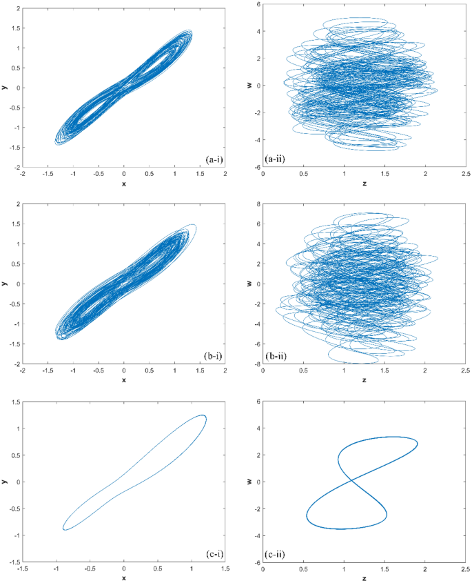
The hyperchaotic attractor of system (1) ((a) hyperchaotic attractor(d = 10); (b) chaotic attractor(d = 17); (c) periodic attractor (d = 22)).
-
If 16 < d ≤ 18, there is one positive Lyapunov exponent, which indicates that system (1) is chaotic. When d = 17, the Lyapunov exponents of system (1) is (0.0932, 0, − 0.0336, − 26.1018), the chaotic attractor is shown in Fig. 3(b);
-
If 18 < d ≤ 27, there are two zero Lyapunov exponents, which indicates that system (1) is quasi-periodic. When d = 22, the Lyapunov exponents of system (1) is (0, 0, − 0.0823, − 25.8783), the periodic orbit attractor is shown in Fig. 3c;
-
If 27 < d ≤ 30, there is one zero Lyapunov exponent, and others are negative, which indicates that system (1) is stable at equilibrium O(0, 0, 0, 0).

Feedback control of the hyperchaotic system
In the control of hyperchaotic systems, linear feedback control has more advantages compared to nonlinear control. Firstly, linear feedback controllers have simple mathematical forms, which are easy to design and implement. Secondly, for certain hyperchaotic systems, linear feedback controllers can achieve global stability of the system, while nonlinear controllers cannot guarantee system stability. Thirdly, linear feedback controllers have a certain robustness to parameter variations within a certain range, while nonlinear controllers may be too sensitive to parameter variations. Finally, the control strategy of linear feedback controllers is easy to interpret, which is beneficial for a deeper understanding of the control mechanism of the system. Therefore, utilizing linear feedback controllers to achieve feedback control of hyperchaotic systems is of greater research significance and value.
In this section, a linear feedback control term into the hyperchaotic system to stabilize it at the equilibrium point O(0, 0, 0, 0). The controlled system of the hyperchaotic system (1) can be defined as:
The Jacobian matrix of the controlled system (2) can be obtained by linearizing around the equilibrium point O(0, 0, 0, 0):
Let det(J0’ − λI) = 0, the eigenvalues of system (2) is calculated at the equilibrium point O(0, 0, 0, 0) as:
If a + k1 > 0, c-k2 < 0, b + k3 > 0, k4 > 0, the λ1 < 0, λ2 < 0, λ3 < 0, λ4 < 0. Using the Routh‐Hurwitz theorem, the system would asymptotically stable to the equilibrium point O(0,0,0,0) when there are only non-negative roots of controlled system (2). The λ1 = − a, λ3 = -b, and they are less than zero if k1 = 0, k3 = 0. Let k2 = 0–20, k4 = 0–20, the maximum Lyapunov exponents of system (2) change by control parameters k2, k4 are shown in Fig. 4. Figure 4 shows that the controlled system (2) would asymptotically stable to the equilibrium point O(0, 0, 0, 0) from the experimental simulation of control parameters k2, k4, when k2 > 12, k4 > 0, here the λ1, λ2, λ3, λ4 are all negatives.

Maximum CLE of the controlled system (2) with k2 and k4.
When a = 35, b = 3, c = 12, d = 10, set the parameters as k1 = 0, k2 = 20, k3 = 0, k4 = 10, then λ1 = -35, λ2 = − 8, λ3 = − 3, λ4 = − 10, and the controlled system (2) would asymptotically stable to the equilibrium point O(0, 0, 0, 0). When the initial values as (10, 10, 5, 5), the changes of the controlled system (2) with time are shown in Fig. 5. The Matlab simulation results show that the state variables in the controlled system (2) will gradually stabilize to the equilibrium point, and the time required from applying control to complete stability is less than 2 s.

The Matlab trajectories of the variables of the controlled system (2).
Multisim simulation results
The electronic circuit simulation software Multisim provides a highly visual simulation environment for hyperchaotic systems, allowing for the effortless creation and adjustment of circuit models and real-time observation of their behavior. This real-time feedback aids in a deeper understanding of the dynamic characteristics of hyperchaotic systems, laying the foundation for simulating the implementation of hyperchaotic systems in embedded hardware.
There are several software programs available for electronic circuit simulation, including PSPICE, LTSPICE, Multisim, and Simulink. In this paper, Multisim is chosen as the industry standard SPICE simulation and circuit design software for analog, digital, and power electronics in education and research.
The output voltages v1, v2, v3 and v4 of the circuit correspond to the four state variables x, y, z and w, respectively. To implement the hyperchaotic system (1), suitable components are selected, and the circuit diagram is shown in Fig. 6.

Circuit diagram for realizing hyperchaotic system (1).
In this study, the circuit is composed of an operational amplifier (LF353N), a multiplier (AD633), linear resistors, and capacitors, with a power supply of ± 15 V. The operational amplifier is utilized for addition, subtraction, and integration of circuits, while the multiplier represents the nonlinearity of the system and connects the four state variables into a unified whole. The electronic circuit equations are obtained based on the hyperchaotic system (1) and are presented below:
Let R0=100kΩ, C0=10nF, t0=R0C0, and x=v1, y=v2, z=v3, w=v4, t=τ/t, the electronic circuit Eq. (3) can be mapped as the dimensionless dynamic system as follows:
Based on the dimensionless system (4), the circuit parameters are chosen as follows: resistor R0 = 100kΩ, capacitor C0 = 10nF, and time t = 1 ms. Where capacitor C = 10nF, resistors R13 = R42 = R1 = 100kΩ, R11 = R12 = R2 = 2.86kΩ, R21 = R3 = 8.33kΩ, R22 = R32 = R5 = 10kΩ, R31 = R4 = 33.33kΩ, R41 = R6 = 3-20kΩ. R6 is adjusted using a potentiometer in Fig. 6 to obtain different values of parameter d.
When d = 10, then R6 = 10kΩ, the phase transition trajectory of hyperchaotic signal is exhibited by an oscilloscope which is shown in Fig. 7a; When d = 17, the R6 = 5.88kΩ, the phase transition trajectory of chaotic signal is shown in Fig. 7b; When d = 22, the R6 = 4.54kΩ, the phase transition trajectory of periodic orbit is shown in Fig. 7c.

The phase portraits of system (3) simulated by Multisim ((a) hyperchaotic phase portraits (R6 = 10kΩ); (b) chaotic phase portraits ((R6 = 5.88kΩ); (c) periodic orbit phase portraits (R6 = 4.54kΩ)).
By utilizing the feedback control theory of the hyperchaotic system in conjunction with the controlled system (2), the electronic circuit Eq. (3), and the dimensionless dynamic system (4). When a = 35, b = 3, c = 12, d = 10, the dimensionless dynamic system of the controlled system as follows:
The values of the electronic components used in the implementation of system (5) are given below: capacitor C = C0 = 10nF, resistor R13 = R42 = R0 = R1 = 100kΩ, R11 = R12 = R2 = 2.86kΩ, R21 = R3 = 8.33kΩ, R22 = R32 = R41 = R43 = R5 = R6 = R8 = 10kΩ, R31 = R4 = 33.33kΩ, R23 = R7 = 5kΩ. Figure 8 shows the Multisim circuit corresponding to the dimensionless power system (5) of the controlled system, contains 7 amplifiers (LF353N), 4 capacitors, 3 multipliers (AD633), and 17 resistors.

Schematic diagram of the controlled system (5).
The trajectories of the variables of the dimensionless power system (5) over time, as simulated in Multisim, are displayed in Fig. 9.

The Multisim trajectories of the variables of the controlled system (5).
The consistency between the results obtained from the electronic circuit simulation software Multisim and the numerical simulation software Matlab provides robust validation for hyperchaotic attractors and linear feedback control of the new hyperchaotic system. Through a meticulous comparison of the output data from both software tools, a remarkably high degree of conformity in the dynamic behavior and evolution trends of attractors under varying conditions has been observed. Consequently, the consistency between numerical simulation results and electronic circuit simulation results not only reinforces the feasibility of the new hyperchaotic system but also furnishes reliable theoretical support for its practical application, establishing a strong foundation for the utilization of new hyperchaotic systems across various domains.
Embedded hardware STM32 implementation results
The embedded hardware STM32 is a 32-bit microcontroller (MCU) based on ARM Cortex-M core, designed for low-power, high-performance, and low-cost embedded applications by STMicroelectronics. STM32 offers high performance, low power consumption, real-time capabilities, cost-effectiveness, and security. This is of great significance for applications requiring audio encryption, real-time signal processing, and complex mathematical computations, such as communication systems, audio storage devices, and speech recognition systems. In comparison to other platforms, it is better suited for applications demanding real-time audio encryption and complex mathematical calculations while maintaining low cost and high programmability.
In this paper, the STM32F103ZET6 is selected for implementing the phase diagram simulation and feedback control of the new hyperchaotic system. The STM32F103ZET operates at a frequency of 72 MHz and incorporates the high-performance ARM Cortex-M3 32-bit RISC core, high-speed embedded memories (Flash memory up to 512 Kbytes and SRAM up to 64 Kbytes), and a wide range of enhanced I/Os and peripherals connected to two APB buses. It has three 12-bit ADCs, one 12-bit DAC, four general-purpose 16-bit timers plus two PWM timers, and several standard and advanced communication interfaces, including two I2Cs, three SPIs, two I2Ss, one SDIO, five USARTs, a USB, and a CAN.
The embedded hardware results are displayed with an oscilloscope, which is Tektronix TBS1072C digital oscilloscope. It is a 2-channel digital storage oscilloscope that has a 70 MHz bandwidth and a sample rate of up to 1 GS/s. The oscilloscope also features a 7-inch WVGA color display that provides clear and detailed visualization of the signals. With these features, the Tektronix TBS1072C is an ideal tool for visualizing the signals generated by the embedded hardware during the experimentation process.
In experiment, the STM32 is used to verify the 4th-order Runge–Kutta method used for the discretization of the new hyperchaotic system (1), the iterative process is shown in Eq. (6). Where a = 35, b = 3, c = 12, d = 10, iteration step h = 0.05. \(\tau \) represents the current moment, \(x\left[\tau \right], y\left[\tau \right], z\left[\tau \right], w\left[\tau \right]\) are the values of the current moment, \({\text{temp\_x}}, \, {\text{temp\_y}}, \, {\text{temp\_z}}, \, {\text{temp\_w}}\) are the intermediate variables, \({\text{h}}_{1}{\text{\_x}}, \, {\text{h}}_{1}{\text{\_y}}, \, {\text{h}}_{1}{\text{\_z}}, \, {\text{h}}_{1}{\text{\_w}}\) are the slopes at the beginning of the time period, \({\text{h}}_{2}{\text{\_x}}, \, {\text{h}}_{2}{\text{\_y}}, \, {\text{h}}_{2}{\text{\_z}}, \, {\text{h}}_{2}{\text{\_w}}\) are the slopes of the midpoint of the time period, the slopes \({\text{h}}_{1}{\text{\_x}}, \, {\text{h}}_{1}{\text{\_y}}, \, {\text{h}}_{1}{\text{\_z}}, \, {\text{h}}_{1}{\text{\_w}}\) are used by Euler's method to determine the values of \(x\left[\tau \right], y\left[\tau \right], z\left[\tau \right], w\left[\tau \right]\) at the point \(\tau \text{+}h/2\), \({\text{h}}_{3}{\text{\_x}}, \, {\text{h}}_{3}{\text{\_y}}, \, {\text{h}}_{3}{\text{\_z}}, \, {\text{h}}_{3}{\text{\_w}}\) are the slopes of the midpoint, but this time the slopes \({\text{h}}_{2}{\text{\_x}}, \, {\text{h}}_{2}{\text{\_y}}, \, {\text{h}}_{2}{\text{\_z}}, \, {\text{h}}_{2}{\text{\_w}}\) are used to determine the \(x\left[\tau \right], y\left[\tau \right], z\left[\tau \right], w\left[\tau \right]\) values, \({\text{h}}_{4}{\text{\_x}}, \, {\text{h}}_{4}{\text{\_y}}, \, {\text{h}}_{4}{\text{\_z}}, \, {\text{h}}_{4}{\text{\_w}}\) are the slopes of the end of the time period, and their \(x\left[\tau \right], y\left[\tau \right], z\left[\tau \right], w\left[\tau \right]\) values are determined by \({\text{h}}_{3}{\text{\_x}}, \, {\text{h}}_{3}{\text{\_y}}, \, {\text{h}}_{3}{\text{\_z}}, \, {\text{h}}_{3}{\text{\_w}}\).
The STM32 generates a discrete hyperchaotic time series, and the DAC converter controls it through SPI to convert digital signals into analog signals, which are then sent to the oscilloscope for display. The platform of the embedded hardware STM32 is illustrated in Fig. 10.

Experimental platform for STM32 implementation.
When d = 10, the phase transition trajectory of hyperchaotic signal is exhibited by an oscilloscope which is shown in Fig. 11a; When d = 17, the phase transition trajectory of chaotic signal is shown in Fig. 11b; When d = 22, the phase transition trajectory of periodic orbit is shown in Fig. 11c.

Experimental results of STM32 implementation ((a) hyperchaotic orbit (d = 10); (b) chaotic orbit (d = 17); (c) periodic orbit (d = 22)).
According to description of Sect. “Feedback control of the hyperchaotic system”, when a = 35, b = 3, c = 12, d = 10, let k1 = 0, k2 = 20, k3 = 0, k4 = 10, then λ1 = − 35, λ2 = − 8, λ3 = − 3, λ4 = − 10, the controlled system (2) would asymptotically stable to the equilibrium point O(0, 0, 0, 0). If the initial values of controlled system (2) as (10,10,5,5), the changes of the controlled system (2) with parameter implemented by STM32 is shown in Fig. 12.

The trajectories of the variables of the controlled system (2) by STM32 implementation.
By comparing the results of Matlab numerical simulation in Fig. 5, the Multisim simulation in Fig. 9, and the STM32 implementation in Fig. 12, it can be seen that the results of all three methods are consistent. However, there may be some numerical accuracy loss due to the digital-to-analog and analog-to-digital conversion processes involved in the DAC output interface of STM32F103ZET and the digital oscilloscope, respectively. Nevertheless, the original characteristics of the hyperchaotic system are preserved.
Audio encryption
In recent years, information security has become a global issue of concern. With the development of mobile internet, personal information, transaction information, and privacy information of netizens are all transmitted through the internet. Due to vulnerabilities in the network transmission process, user information leakage has become a significant security risk. Therefore, to solve this problem, it is necessary to use information encryption technology.
Confusion and diffusion are two common encryption techniques. Confusion typically refers to increasing the complexity of the ciphertext by using complex substitution rules or mixing the key with the plaintext. Diffusion involves ensuring that changes in individual plaintext bits propagate throughout the ciphertext so that even small changes in the plaintext result in significant differences in the ciphertext. In this paper, the audio encryption based on hyperchaotic sequences studied falls under the category of confusion methods.
Chaos encryption has become a research hotspot in information encryption due to its nonlinearity, real-time performance, security, anti-interference, and short key length. However, compared with chaotic encryption, hyperchaotic encryption has the following advantages:
-
a.
Higher security. Hyperchaotic systems have more complex dynamical behavior, and the output key sequence has higher randomness and unpredictability, thereby improving the security of the encryption system.
-
b.
Higher anti-interference. The key sequence output by the hyperchaotic system has a higher range and frequency of disturbance, which can effectively resist common attack methods such as noise attacks and interference attacks.
-
c.
Better scalability. Hyperchaotic systems can achieve high-dimensional expansion, that is, multiple chaotic systems' functions can be implemented in a hyperchaotic system, making it applicable to more complex encryption systems.
-
d.
Stronger self-synchronization. The key sequence output by the hyperchaotic system can automatically synchronize during the encryption and decryption process without external synchronization control, making the encryption system simpler and more practical.
In this section, the audio encryption algorithm based on the hyperchaotic key sequence is studied, using the 4D hyperchaotic system that has been constructed. Then designed a method to generate hyperchaotic key sequence, and implemented audio encryption using the cross-XOR operation. The experiment was conducted and validated on the embedded hardware STM32.
Hyperchaotic key sequence
Due to the high randomness and complexity of the hyperchaotic system, the security of the encryption algorithm is enhanced. The generation of hyperchaotic key sequence transforms the hyperchaotic sequence into the required form of the key sequence through a specific quantization algorithm. The steps are as follows:
Step 1: Pre-iterate the hyperchaotic system N1 times to eliminate the transient effects of the hyperchaotic system entering a hyperchaotic state.
Step 2: Iterate the hyperchaotic system N2 times to generate a new set of state values A = {Ax, Ay, Az, Aw}, where Ax = {x1, x2, x3, …, xk}, Ay = {y1, y2, y3, …, yk}, Az = {z1, z2, z3, …, zk}, and Aw = {w1, w2, w3, …, wk}, 0 < k ≤ N2. Then, scale down the state values A down to 1/p and take q decimal places to generate the new state values B = {Bx, By, Bz, Bw}, where Bx = {bx1, bx2, bx3, …, bxk}, By = {by1, by2, by3, …, byk}, Bz = {bz1, bz2, bz3, …, bzk}, and Bw = {bw1, bw2, bw3, …, bwk}. The conversion formula is as follows:
where floor(∙) denotes the floor function, and p and q are adjustable parameters, where p represents scaling down the value by 1/p, and q represents taking q decimal places as the new state value.
Step 3: Calculate the key sequence. According to the positive and negative changes in the numerical value of the state value A, adjust the order of the state value B to generate the key sequence K = {K1, K2, K3, …, Kk}. The mapping relationship between the sorting rule of state value A, B and the generation of key sequence K is shown in Table 1.
Step 4: Repeat steps 2 and 3 for (Frame_Len/4–1) times to generate a key matrix K with a length of (Frame_Len*4), where Frame_Len is the length of one frame of audio data.
Cross-XOR operation
To demonstrate the simplicity and non-linearity advantages of implementing super-chaotic keys, and to fully utilize the advantages of ciphertext interleaving diffusion technology in audio encryption and improve its ability to resist illegal attacks, a new method of cross-XOR operation is introduced. Its features are suitable for audio signal encryption, non-linear ciphertext, easy to implement, can improve the speed of ciphertext diffusion.
Assuming that the audio sequence S and key sequence K are m-bit binary sequences, that is, S = {s1,s2,s3,…,sm}, K = {k1,k2,k3,…,km}, SH and SL represent the high m/2-bit and low m/2-bit sub-sequences of the audio sequence S, and KH and KL represent the high m/2-bit and low m/2-bit sub-sequences of the key sequence K. The implementation of audio encryption based on cross-XOR operation is shown in the following equation:
where R sequence is the result of audio encryption using cross-XOR operation, where RH and RL represent the high m/2-bit and low m/2-bit sub-sequences of the key sequence R. The audio decryption is the inverse operation of encryption, which is implemented as shown in the following equation:
where S' sequence is the result of audio decryption using cross-XOR operation, where S'H and S'L represent the high m/2-bit and low m/2-bit sub-sequences of the key sequence S'. The audio encryption and decryption processes based on cross-XOR operation are shown in Fig. 13.

Block diagrams of cross-XOR operation and its audio encryption and decryption processes.
Experimental results
In this experiment, the embedded hardware STM32F103ZET6 was used to implement audio encryption based on the hyperchaotic key sequence. Since the embedded hardware STM32F103ZET6 does not integrate an audio acquisition module and display, the data input is imported into the embedded hardware STM32 in the form of a list. The output of the encrypted and decrypted audio sequences is exported to the PC through the serial port of the embedded hardware STM32F103ZET6, and then printed out using a serial port debugging tool, as shown in Fig. 14. Figure 15 is the hyperchaotic key sequence.

The encrypted and decrypted sequences printed by the serial port debugging tool.

Hyperchaotic key sequence.
The data sequence output by the embedded hardware STM32F103ZET6 serial port is transmitted to the PC through the serial port, and the audio sequence is displayed using Matlab, as shown in Figs. 16 and 17.

Time domain data before and after audio encryption.

Spectrograms of the audio sequence before and after encryption.
Figure 16a shows the original audio data in the time domain before encryption, Fig. 16b shows the encrypted audio data in the time domain, and Fig. 16c shows the decrypted audio data in the time domain. By comparing Fig. 16a and c, it shows that the time domain data of the audio sequence before and after encryption is identical, which indicates that the hyperchaotic key sequence did not cause distortion to the audio data. At the same time, from Fig. 16b, it shows that the time domain distribution of the audio sequence after encryption with the hyperchaotic key sequence is completely chaotic and different from the time domain pattern of the original audio data. This demonstrates that the encrypted ciphertext has completely concealed the characteristic information of the original audio data.
Figure 17 shows the spectrograms of the audio signal before encryption, after encryption, and after decryption. In Fig. 17b, it is evident that the encrypted audio signal exhibits a wide frequency distribution, resembling random noise in the time–frequency domain. Comparing Fig. 17a and c, the frequency domain information remains consistent before and after audio signal encryption. This implies that the decrypted audio signal maintains its original characteristics without any distortion, confirming the effectiveness of the hyperchaotic sequence encryption.
Conclusions
In this paper, a new 4D hyperchaotic system is proposed, and its basic dynamic behavior is analyzed, including its chaotic attractor, equilibrium point stability, Lyapunov exponent spectrum, bifurcation diagram, and so on. The study demonstrates that the system has only one equilibrium point and remains hyperchaotic by varying its parameters over a wide range. A linear feedback control approach is introduced to stabilize the hyperchaotic system to its equilibrium point, and the effectiveness of this approach is proven through both Multisim circuit simulation and embedded hardware STM32 implementation.
Furthermore, the designed hyperchaotic system is applied to audio encryption in this paper. The audio encryption algorithm employs the cross-XOR operation method, which is simple to implement and has a certain degree of complexity. The experimental results show that the encrypted audio sequence is identical to the original sequence in the time domain, while it appears as random noise in the frequency domain, making it impossible to discern the actual information carried by the audio. This proves the effectiveness of the cross-XOR operation method based on hyperchaotic key sequence for audio encryption.
In future work, the high complexity of the hyperchaotic key sequence will be leveraged to study the master–slave mode of data encryption and decryption using embedded hardware STM32, which has significant research value in areas such as image encryption, audio encryption, video encryption, and more.
Data availability
The data used to support the findings of this study are available from the corresponding author upon request.
References
Rössler, O. E. An equation for continuous chaos. Phys. Lett. A 57, 397–398. https://doi.org/10.1016/0375-9601(76)90101-8 (1976).
Vaidyanathan, S. et al. A new 4-D hyperchaotic two-scroll system with hidden attractor and its field-programmable gate array implementation. Int. J. Circuit Theory Appl. https://doi.org/10.1002/cta.3700 (2023).
Liu, Y., Zhou, Y. & Guo, B. Hopf bifurcation, periodic solutions, and control of a new 4d hyperchaotic system. Mathematics 11, 2699. https://doi.org/10.3390/math11122699 (2023).
Zhang, Z. et al. Construction of a family of 5D Hamiltonian conservative hyperchaotic systems with multistability. Physica A Stat. Mech. Appl. 620, 128759. https://doi.org/10.1016/j.physa.2023.128759 (2023).
Wang, E., Yan, S., Sun, X. & Wang, Q. Analysis of bifurcation mechanism of new hyperchaotic system, circuit implementation, and synchronization. Nonlinear Dyn. 111, 3869–3885. https://doi.org/10.1007/s11071-022-08034-w (2023).
El-Dessoky, M. M., Alzahrani, E. & Al-Rehily, N. Control and adaptive modified function projective synchronization of a new hyperchaotic system. Alex. Eng. J. 60, 3985–3990. https://doi.org/10.1016/j.aej.2021.02.059 (2021).
Liu, X., Tong, X., Zhang, M. & Wang, Z. A highly secure image encryption algorithm based on conservative hyperchaotic system and dynamic biogenetic gene algorithms. Chaos Solitons Fractals 171, 113450. https://doi.org/10.1016/j.chaos.2023.113450 (2023).
Arellano-Delgado, A., Méndez-Ramírez, R. D., López-Gutiérrez, R. M., Murillo-Escobar, M. A. & Cruz-Hernández, C. Enhancing the emergence of hyperchaos using an indirect coupling and its verification based on digital implementation. Nonlinear Dyn. 111, 9591–9605. https://doi.org/10.1007/s11071-023-08313-0 (2023).
Sangpet, T. & Kuntanapreeda, S. Finite-time synchronization of hyperchaotic systems based on feedback passivation. Chaos Solitons Fractals 132, 109605. https://doi.org/10.1016/j.chaos.2020.109605 (2020).
Wang, X.-Y., Wang, X.-L., Teng, L., Jiang, D.-H. & Xian, Y. Lossless embedding: A visually meaningful image encryption algorithm based on hyperchaos and compressive sensing. Chin. Phys. B 32, 020503. https://doi.org/10.1088/1674-1056/aca149 (2023).
Wang, X., Min, X., Zhou, P. & Yu, D. Hyperchaotic circuit based on memristor feedback with multistability and symmetries. Complexity 2020, 1–10. https://doi.org/10.1155/2020/2620375 (2020).
Ren, L., Lin, M. H., Abdulwahab, A., Ma, J. & Saberi-Nik, H. Global dynamical analysis of the integer and fractional 4D hyperchaotic Rabinovich system. Chaos Solitons Fractals 169, 113275. https://doi.org/10.1016/j.chaos.2023.113275 (2023).
Li, H., Shen, Y., Han, Y., Dong, J. & Li, J. Determining Lyapunov exponents of fractional-order systems: A general method based on memory principle. Chaos Solitons Fractals 168, 113167. https://doi.org/10.1016/j.chaos.2023.113167 (2023).
Xiao, Y., Sun, K., Yu, M. & Xu, X. Dynamics of a new multi-cavity hyperchaotic map and its DSP implementation. Int. J. Bifurc. Chaos 29, 1950194. https://doi.org/10.1142/S0218127419501943 (2019).
Liu, T. et al. Hyperchaotic maps of a discrete memristor coupled to trigonometric function. Physica Scripta 96, 125242. https://doi.org/10.1088/1402-4896/ac3153 (2021).
Leutcho, G. D. et al. Dynamics of a new multistable 4D hyperchaotic lorenz system and its applications. Int. J. Bifurc. Chaos https://doi.org/10.1142/S0218127422500018 (2022).
Xiao, Y., Sun, K. & He, S. Constructing chaotic map with multi-cavity. Eur. Phys. J. Plus https://doi.org/10.1140/epjp/s13360-019-00052-9 (2020).
Cui, N. & Li, J. A new 4D hyperchaotic system and its control. AIMS Math. 8, 905–923. https://doi.org/10.3934/math.2023044 (2023).
Liu, X., Bi, X., Yan, H. & Mou, J. A chaotic oscillator based on meminductor, memcapacitor, and memristor. Complexity 2021, 1–16. https://doi.org/10.1155/2021/7223557 (2021).
Yu, F. et al. Dynamics analysis, FPGA realization and image encryption application of a 5D memristive exponential hyperchaotic system. Integration 90, 58–70. https://doi.org/10.1016/j.vlsi.2023.01.006 (2023).
Yu, F. et al. Dynamic analysis and FPGA implementation of a new, simple 5D Memristive hyperchaotic sprott-C system. Mathematics 11, 701. https://doi.org/10.3390/math11030701 (2023).
Prakash, P. et al. A novel simple 4-D hyperchaotic system with a saddle-point index-2 equilibrium point and multistability: Design and FPGA-based applications. Circuits Syst. Signal Process. 39, 4259–4280. https://doi.org/10.1007/s00034-020-01367-0 (2020).
Jia, S. H., Li, Y. X., Shi, Q. Y. & Huang, X. Design and FPGA implementation of a memristor-based multi-scroll hyperchaotic system. Chin. Phys. B 31, 070505. https://doi.org/10.1088/1674-1056/ac4a71 (2022).
Vaidyanathan, S., Tlelo-Cuautle, E., Sambas, A., Dolvis, L. G. & Guillén-Fernández, O. FPGA design and circuit implementation of a new four-dimensional multistable hyperchaotic system with coexisting attractors. Int. J. Comput. Appl. Technol. 64, 223–234. https://doi.org/10.1504/IJCAT.2020.111848 (2020).
Jiao, X., Dong, E. & Wang, Z. Dynamic analysis and FPGA implementation of a Kolmogorov-like hyperchaotic system. Int. J. Bifurc. Chaos 31, 2150052. https://doi.org/10.1142/S0218127421500528 (2021).
Yan, S., Wang, E., Wang, Q., Sun, X. & Ren, Y. Analysis, circuit implementation and synchronization control of a hyperchaotic system. Physica Scripta 96, 125257. https://doi.org/10.1088/1402-4896/ac379b (2021).
Wang, X., Pham, V. T. & Volos, C. Dynamics, circuit design, and synchronization of a new chaotic system with closed curve equilibrium. Complexity 2017, 1–9. https://doi.org/10.1155/2017/7138971 (2017).
Al-Khedhairi, A., Elsonbaty, A., Abdel Kader, A. H. & Elsadany, A. A. Dynamic analysis and circuit implementation of a new 4D Lorenz-type hyperchaotic system. Math. Probl. Eng. 2019, 1–17. https://doi.org/10.1155/2019/6581586 (2019).
Jiang, Z. & Liu, X. Image encryption algorithm based on discrete quantum baker map and chen hyperchaotic system. Int. J. Theor. Phys. https://doi.org/10.1007/s10773-023-05277-0 (2023).
Nestor, T. et al. A new 4D hyperchaotic system with dynamics analysis, synchronization, and application to image encryption. Symmetry 14, 424. https://doi.org/10.3390/sym14020424 (2022).
Vaidyanathan, S. et al. A new 4-D multi-stable hyperchaotic system with no balance point: Bifurcation analysis, circuit simulation, FPGA realization and image cryptosystem. IEEE Access 9, 144555–144573. https://doi.org/10.1109/ACCESS.2021.3121428 (2021).
Sun, S. & Guo, Y. A new hyperchaotic image encryption algorithm based on stochastic signals. IEEE Access https://doi.org/10.1109/ACCESS.2021.3121588 (2021).
Gui, X., Huang, J., Li, L., Li, S. & Cao, J. A novel hyperchaotic image encryption algorithm with simultaneous shuffling and diffusion. Multim. Tools Appl. 81, 21975–21994. https://doi.org/10.1007/s11042-022-12239-x (2022).
Zeng, J. & Wang, C. A novel hyperchaotic image encryption system based on particle swarm optimization algorithm and cellular automata. Secur. Commun. Netw. 2021, 1–15. https://doi.org/10.1155/2021/6675565 (2021).
Xu, J. & Zhao, B. Designing an image encryption algorithm based on hyperchaotic system and DCT. Int. J. Bifurc. Chaos https://doi.org/10.1142/S0218127423500219 (2023).
Lin, R. & Li, S. An image encryption scheme based on lorenz hyperchaotic system and RSA algorithm. Secur. Commun. Netw. 2021, 1–18. https://doi.org/10.1155/2021/5586959 (2021).
Alibraheemi, H. M. M., Al-Gayem, Q. & Hussein, E. A. R. Four dimensional hyperchaotic communication system based on dynamic feedback synchronization technique for image encryption systems. Int. J. Electr. Comput. Eng. 12, 957–965. https://doi.org/10.11591/ijece.v12i1.pp957-965 (2022).
Wang, L. & Chen, Z. Hyperchaotic image encryption algorithm based on BD-Zigzag transformation and DNA coding. In Lecture Notes in Electrical Engineering (eds Liu, Q. et al.) 667–677 (Springer Nature Singapore, 2022). https://doi.org/10.1007/978-981-19-6901-0_69.
Hosny, K. M., Kamal, S. T., Darwish, M. M. & Papakostas, G. A. New image encryption algorithm using hyperchaotic system and fibonacci q-matrix. Electronics (Switzerland) 10, 1066. https://doi.org/10.3390/electronics10091066 (2021).
Ahmad, M., Doja, M. N. & Beg, M. M. S. Security analysis and enhancements of an image cryptosystem based on hyperchaotic system. J. King Saud Univ. Comput. Inform. Sci. 33, 77–85. https://doi.org/10.1016/j.jksuci.2018.02.002 (2021).
Sun, J., Cai, H., Gao, Z., Wang, C. & Zhang, H. A novel non-equilibrium hyperchaotic system and application on color image steganography with FPGA implementation. Nonlinear Dyn. 111, 3851–3868. https://doi.org/10.1007/s11071-022-07993-4 (2023).
Ameen, M. J. M. & Hreshee, S. S. Securing physical layer of 5G wireless network system over GFDM using linear precoding algorithm for massive MIMO and hyperchaotic QRDecomposition. Int. J. Intell. Eng. Syst. 15, 579–591. https://doi.org/10.22266/ijies2022.1031.50 (2022).
Naik, R. B. & Singh, U. A review on applications of chaotic maps in pseudo-random number generators and encryption. Ann Data Sci. https://doi.org/10.1007/s40745-021-00364-7 (2022).
Abdulkadhim, H. A. & Shehab, J. N. Audio steganography based on least significant bits algorithm with 4D grid multi-wing hyper-chaotic system. Int. J. Electr. Comput. Eng. 12, 320–330. https://doi.org/10.11591/ijece.v12i1.pp320-330 (2022).
Singh, J. P., Sarkar, A. B. & Roy, B. K. A better and robust secure communication using a highly complex hyperchaotic system. Iran. J. Sci. Technol. Trans. Electr. Eng. https://doi.org/10.1007/s40998-023-00593-x (2023).
Hammami, S. Multi-switching combination synchronization of discrete-time hyperchaotic systems for encrypted audio communication. IMA J. Math. Control Inform. 36, 583–602. https://doi.org/10.1093/imamci/dnx058 (2019).
Sharma, C., Bagga, A., Singh, B. K. & Shabaz, M. A novel optimized graph-based transform watermarking technique to address security issues in real-time application. Math. Probl. Eng. 2021, 1–27. https://doi.org/10.1155/2021/5580098 (2021).
Gayathri, D. & PushpaLakshmi, R. A high order video compressive sensing encryption using fractional order hyper chaotic system with intelligent scrambling and nucleotide sequences. J. Pharm. Negat. Results 13, 1939–1951. https://doi.org/10.47750/pnr.2022.13.S07.266 (2022).
Liu, S., Li, Y., Ge, X., Li, C. & Zhao, Y. A novel hyperchaotic map and its application in fast video encryption. Physica Scripta 97, 085210. https://doi.org/10.1088/1402-4896/ac7c43 (2022).
Arthi, G., Thanikaiselvan, V. & Amirtharajan, R. 4D Hyperchaotic map and DNA encoding combined image encryption for secure communication. Multim. Tools Appl. 81, 15859–15878. https://doi.org/10.1007/s11042-022-12598-5 (2022).
Wei, C. & Li, G. Encryption algorithm of video images combining hyper-chaotic system and logistic mapping. Jisuanji Gongcheng/Comput. Eng. 48, 263–271. https://doi.org/10.19678/j.issn.1000-3428.0061608 (2022).
Huang, H. & Cheng, D. A secure image compression-encryption algorithm using DCT and hyperchaotic system. Multim. Tools Appl. 81, 31329–31347. https://doi.org/10.1007/s11042-021-11796-x (2022).
Li, X. et al. Video encryption based on hyperchaotic system. Multim. Tools Appl. 79, 23995–24011. https://doi.org/10.1007/s11042-020-09200-1 (2020).
Meng, Q., Wang, X., Qi, Z. & Zhang, Y. Multiple parameters weighted-type FRactional fourier transform secure communication method based on cosine power-activation discrete hyperchaotic encryption. Dianzi Yu Xinxi Xuebao/J. Electron. Inform. Technol. 45, 1688–1696. https://doi.org/10.11999/JEIT220364 (2023).
Kadhim, M. W., Kafi, D. A., Abed, E. A. & Jamal, R. K. A novel technique in encryption information based on Chaos–hologram. J. Optics (India) https://doi.org/10.1007/s12596-022-01087-5 (2023).
Fan, C. & Ding, Q. Coexisting point attractors, multi-transient behaviors, area-preserving chaotic systems, non-degenerate hyperchaotic systems derived from a simple 3D discrete system. Physica Scripta 98, 055206. https://doi.org/10.1088/1402-4896/acc89d (2023).
Wen, H. et al. Secure optical image communication using double random transformation and memristive chaos. IEEE Photonics J. 15, 1–11. https://doi.org/10.1109/JPHOT.2022.3233129 (2023).
Khan, M. Z., Sarkar, A. & Noorwali, A. Memristive hyperchaotic system-based complex-valued artificial neural synchronization for secured communication in Industrial Internet of Things. Eng. Appl. Artif. Intell. 123, 106357. https://doi.org/10.1016/j.engappai.2023.106357 (2023).
Abed, E. A., Mousa, S. K. & Jamal, R. K. A novel secure communication system using optoelectronic feedback in semiconductor laser. J. Optics (India) https://doi.org/10.1007/s12596-023-01182-1 (2023).
Zhang, Y., Bao, H., Hua, Z. & Huang, H. Two-dimensional exponential chaotic system with hardware implementation. IEEE Trans. Ind. Electron. 70, 9346–9356. https://doi.org/10.1109/TIE.2022.3206747 (2023).
He, J., Qiu, W. & Cai, J. Synchronization of hyperchaotic systems based on intermittent control and its application in secure communication. J. Adv. Computat. Intell. Intell. Inform. 27, 292–303. https://doi.org/10.20965/jaciii.2023.p0292 (2023).
Shen, Y. et al. Fast and secure image encryption algorithm with simultaneous shuffling and diffusion based on a time-delayed combinatorial hyperchaos map. Entropy 25, 753. https://doi.org/10.3390/e25050753 (2023).
Zeng, J. et al. A new method for constructing discrete hyperchaotic systems with a controllable range of Lyapunov exponents and its application in information security. Physica Scripta 98, 075212. https://doi.org/10.1088/1402-4896/acd887 (2023).
Lü, J. & Chen, G. A new chaotic attractor coined. Int. J. Bifurc. Chaos Appl. Sci. Eng. 12, 659–661. https://doi.org/10.1142/S0218127402004620 (2002).
Acknowledgements
Thanks professor P. Zhou for valuable suggestion. This work was supported by Science and Technology Project of Chongqing Municipal Education Commission (Grant No. KJZD-K202303301, KJQN202201630, KJQN202203309 and KJQN202203308).
Author information
Authors and Affiliations
Contributions
Conceptualization, X.F.C. and S.M.F.; methodology, X.F.C. and S.M.F.; software, X.F.C.; validation, X.F.C., J.L. and S.M.F.; formal analysis, X.F.C.; investigation, S.M.F.; resources, X.F.C., J.L. and S.M.F.; data curation, J.L.; writing—original draft preparation, X.F.C.; writing—review and editing, J.L.; supervision, X.F.C. and S.M.F.; project administration, S.M.F.; funding acquisition, X.F.C. and S.M.F. All authors reviewed the manuscript.
Corresponding author
Ethics declarations
Competing interests
The authors declare no competing interests.
Additional information
Publisher's note
Springer Nature remains neutral with regard to jurisdictional claims in published maps and institutional affiliations.
Rights and permissions
Open Access This article is licensed under a Creative Commons Attribution 4.0 International License, which permits use, sharing, adaptation, distribution and reproduction in any medium or format, as long as you give appropriate credit to the original author(s) and the source, provide a link to the Creative Commons licence, and indicate if changes were made. The images or other third party material in this article are included in the article's Creative Commons licence, unless indicated otherwise in a credit line to the material. If material is not included in the article's Creative Commons licence and your intended use is not permitted by statutory regulation or exceeds the permitted use, you will need to obtain permission directly from the copyright holder. To view a copy of this licence, visit http://creativecommons.org/licenses/by/4.0/.
About this article

Cite this article
Fu, S., Cheng, X. & Liu, J. Dynamics, circuit design, feedback control of a new hyperchaotic system and its application in audio encryption. Sci Rep 13, 19385 (2023). https://doi.org/10.1038/s41598-023-46161-5
Received:
Accepted:
Published:
DOI: https://doi.org/10.1038/s41598-023-46161-5
This article is cited by
-
An audio encryption algorithm based on a non-degenerate 2D integer domain hyper chaotic map over GF(2n)
Multimedia Tools and Applications (2024)
Comments
By submitting a comment you agree to abide by our Terms and Community Guidelines. If you find something abusive or that does not comply with our terms or guidelines please flag it as inappropriate.
