
Abstract
Develoment of image recognition AI algorithms for flower-visiting arthropods has the potential to revolutionize the way we monitor pollinators. Ecologists need light-weight models that can be deployed in a field setting and can classify with high accuracy. We tested the performance of three deep learning light-weight models, YOLOv5nano, YOLOv5small, and YOLOv7tiny, at object recognition and classification in real time on eight groups of flower-visiting arthropods using open-source image data. These eight groups contained four orders of insects that are known to perform the majority of pollination services in Europe (Hymenoptera, Diptera, Coleoptera, Lepidoptera) as well as other arthropod groups that can be seen on flowers but are not typically considered pollinators (e.g., spiders-Araneae). All three models had high accuracy, ranging from 93 to 97%. Intersection over union (IoU) depended on the relative area of the bounding box, and the models performed best when a single arthropod comprised a large portion of the image and worst when multiple small arthropods were together in a single image. The model could accurately distinguish flies in the family Syrphidae from the Hymenoptera that they are known to mimic. These results reveal the capability of existing YOLO models to contribute to pollination monitoring.
Introduction
Most crops and wild plant species rely on interactions with animal pollinators for reproduction1. Pollination is therefore a critical ecosystem services, which has an annual market value of more than $237 billion2. The threats to pollinators are not fully understood, which has led to urgent calls for more studies aimed at understanding how pollinators and plant-pollinator interactions change across environmental gradients (EU Pollinators Initiative, EC 2018).
Currently, most data on plant-pollinator interactions are acquired from field observations and collections of pollinators contacting reproductive parts of flowers. The identification of pollinators is a time-consuming step in this research. For example, it is typical for pollination ecologists to spend weeks in the field collecting observational data and arthropods, and many weeks or months afterwards pinning, sorting and identifying those arthropods using microscopy or DNA barcoding2,3,4. AI tools, in particular convolutional neural networks (CNNs) for image classification, have the potential to allow for efficient identification of plant-pollinator interactions from field images. Training these tools require a vast amount of annotated data, which can be met with the growing amount of digital data from citizen science platforms and media platforms that have been curated by taxonomic experts5,6.
Developments of applications for automated recognition have resulted in some outstanding products for plant identification, due to the consolidation of different machine learning methods7,8, the increase in image data availability9, and advances in computer hardware over the past decade. For example, the Flora Incognita app can currently distinguish more than 16,000 European plant species from images taken by citizens. Like plants, automated arthropod identification is challenged by the vast number of taxa to be classified, by the complexity of image backgrounds and variability in shooting angles, and by the fact that individuals of the same taxa vary in their morphology and individuals of different taxa sometimes look very similar6,8. Arthropod identification is also challenged by dealing with multiple individuals that overlap in the same image, different lighting conditions6,10,11, arthropods that blend in cluttered backgrounds, individuals that move very fast and/or are hidden by parts of plants12, and dramatic size differences between arthropod species.
Deep learning has revolutionized computer vision in many fields of natural sciences, such as medicine13,14, and remote sensing15,16,17. In the field of automatic identification of arthropods, convolutional neural networks (CNN) used for image classification are still in a pre-mature phase. However, it is acknowledged that they have the potential to revolutionize data collection11,18. The development of AI tools for arthropod classification started with a focus on particular taxa and/or the identification of museum specimens with a homogeneous image background. For example, pictures taken of arthropod wings in controlled settings (i.e., under the microscope) can identify several groups of bees19, butterflies20,21 and syrphid flies22. The application of CNNs on arthropod identification ranges from a few to multiple taxa and considers a growing number of images, for example, nine tiger beetles genera and 380 images23, nine groups of arthropods and nearly 2000 images24, ten butterfly species and nearly 18,000 images21, 36 bumble bee species and nearly 90,000 images6. Progress in this direction was carried out also in the citizen science and private sectors with the ongoing research in mobile apps like Seek, ObsIdentify, NABU Insektensommer and Google Lens.
Recent developments in camera hardware and image recognition have been applied to study insect pollination, typically focused on a single plant species or a single pollinator species. For example, Bjerge and colleagues25 use a custom camera system and CNNs to capture images and classify broad groups of arthropods that visit plants in the genus Sedum. Ratnayake and colleagues12,26 used Raspberry Pi hardware and CNNs to track the movement of individual honeybees, allowing for spatial monitoring and behavioral analysis of this important pollinator species in an agricultural setting. Several studies have introduced low-cost and open-source camera trap systems that are enabling efficient collection of insect images in field settings27,28,29. However, there is a need to develop tools that can classify flower-visiting arthropods that visit a wide variety of flowers in a broad geographic region, such as Europe.
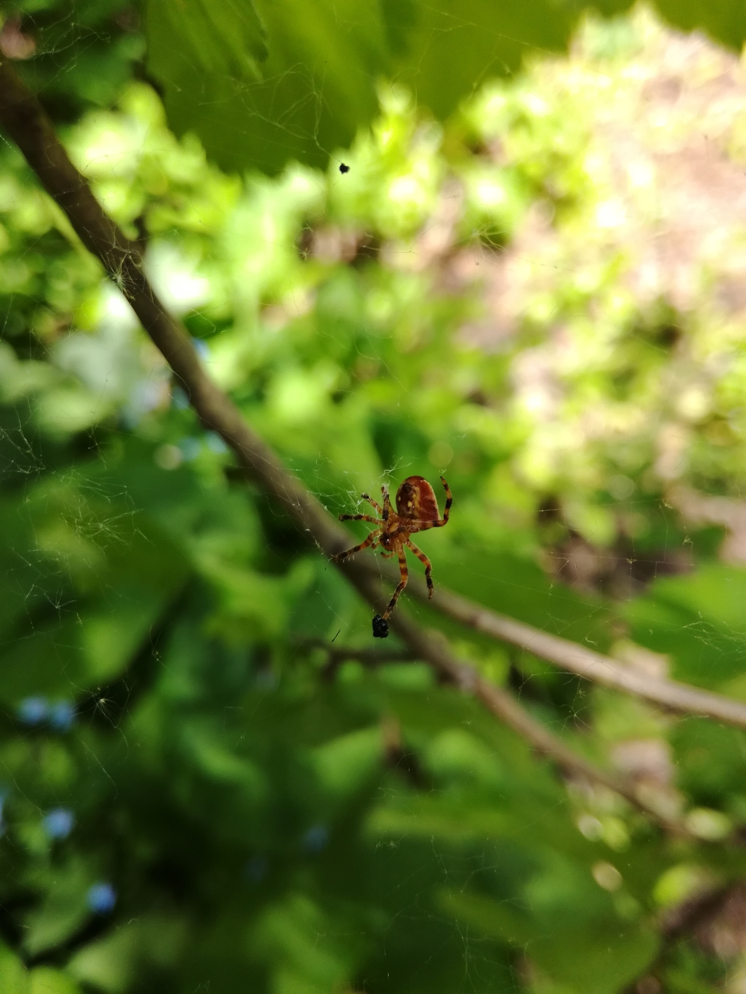
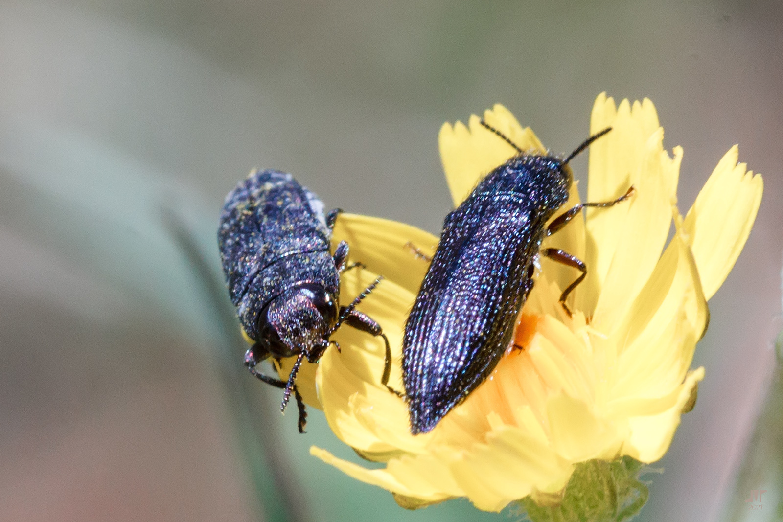
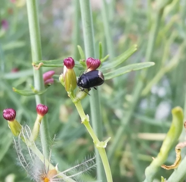
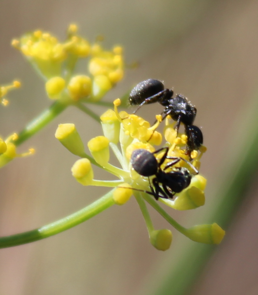
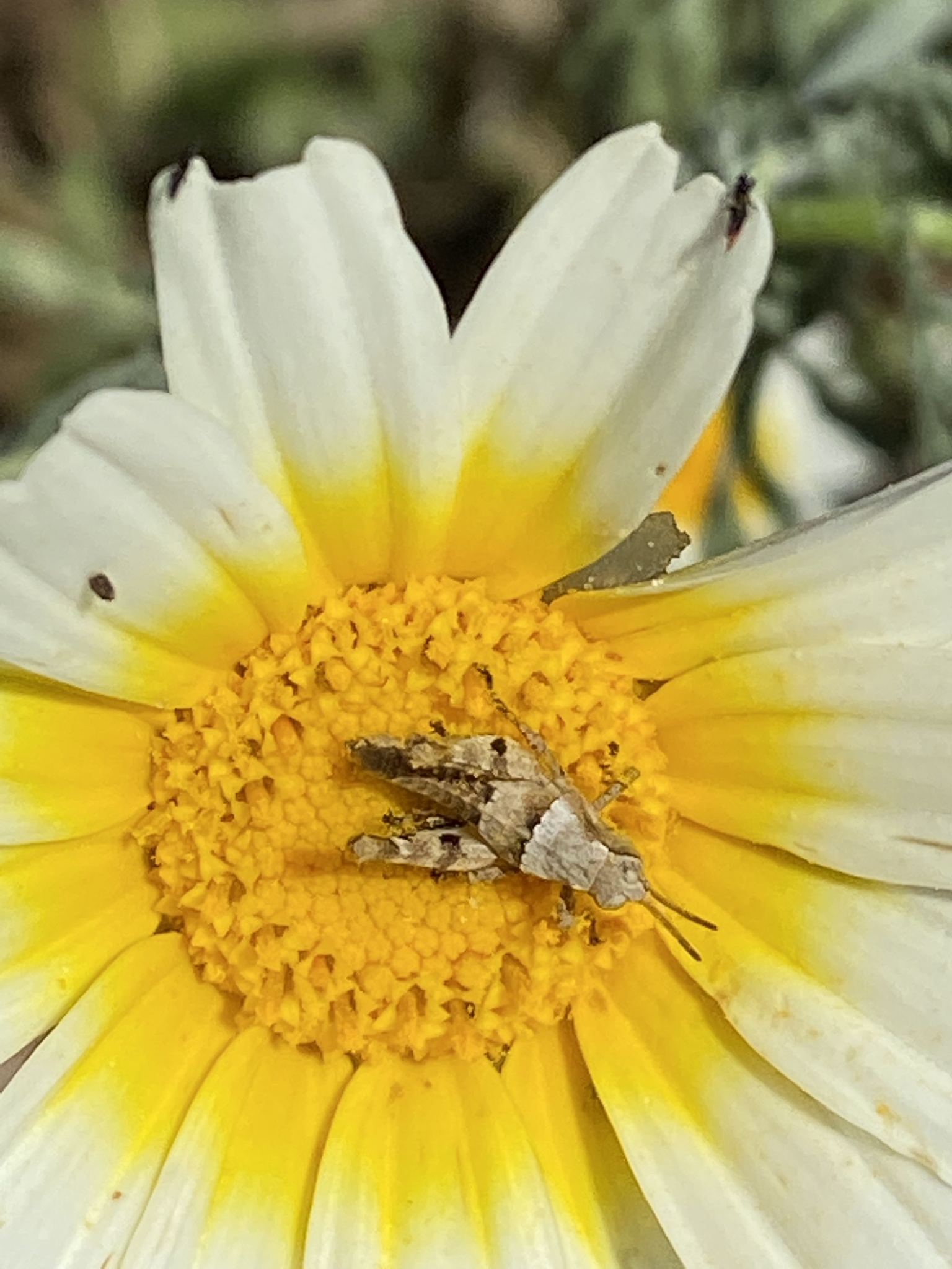
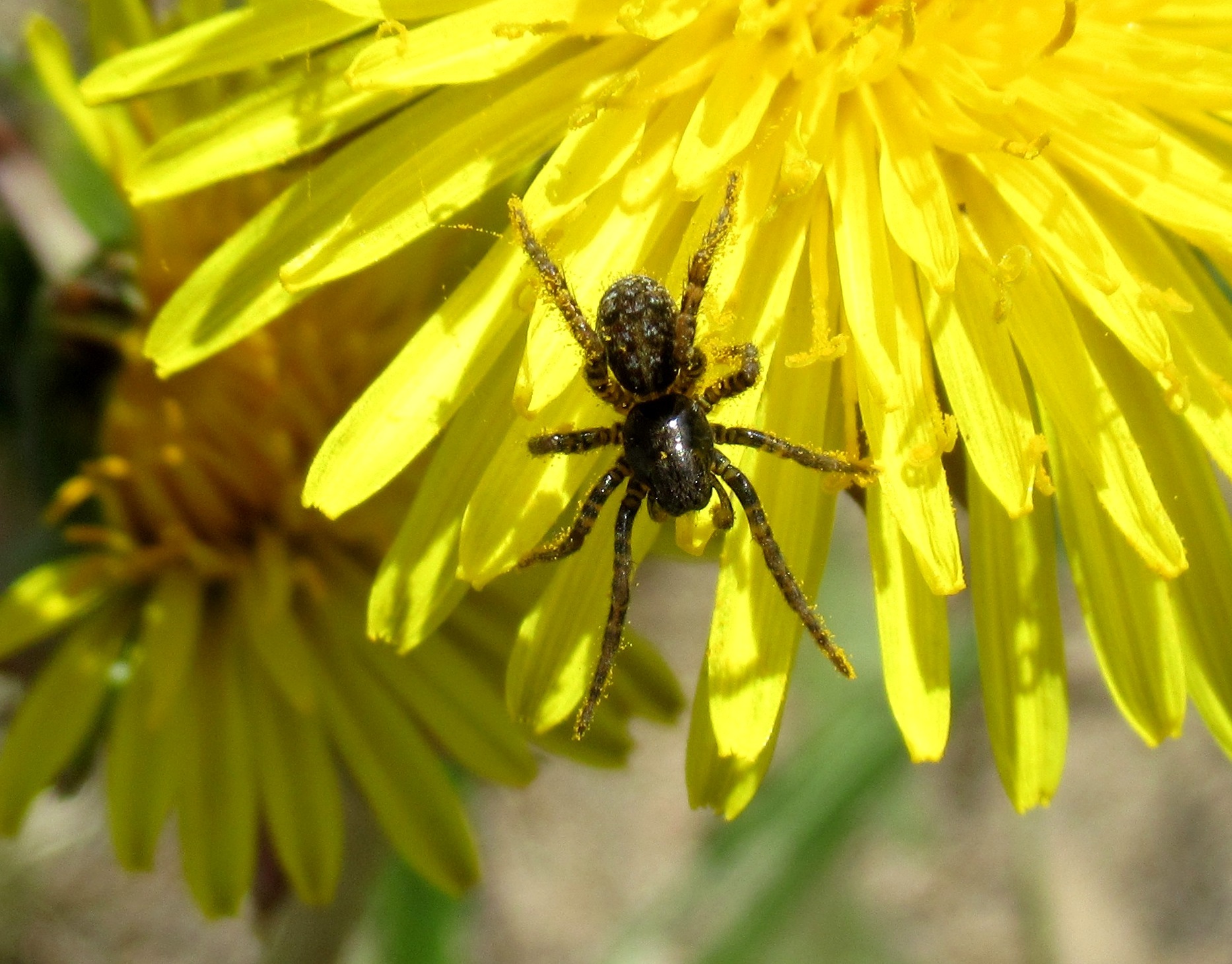
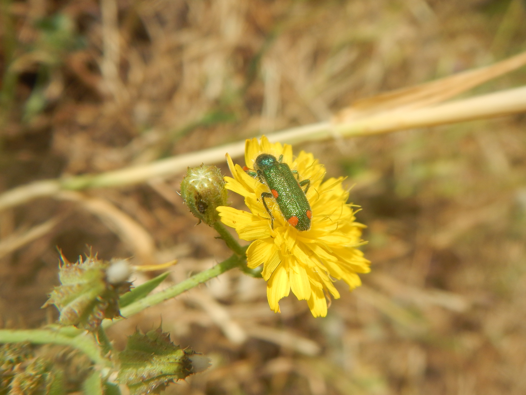
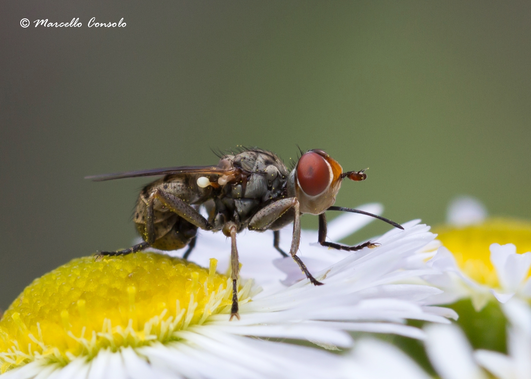
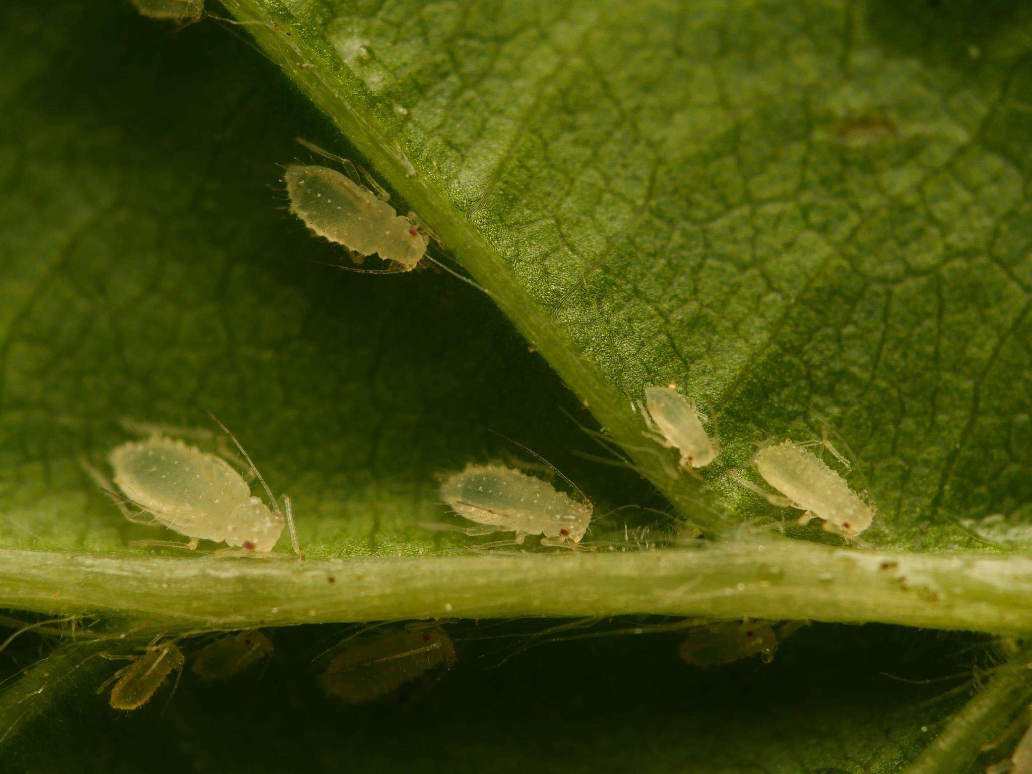
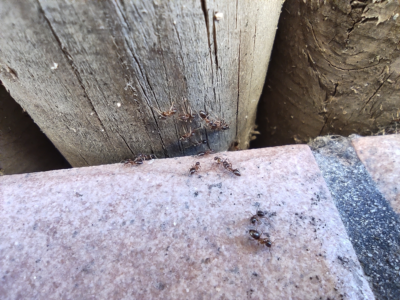
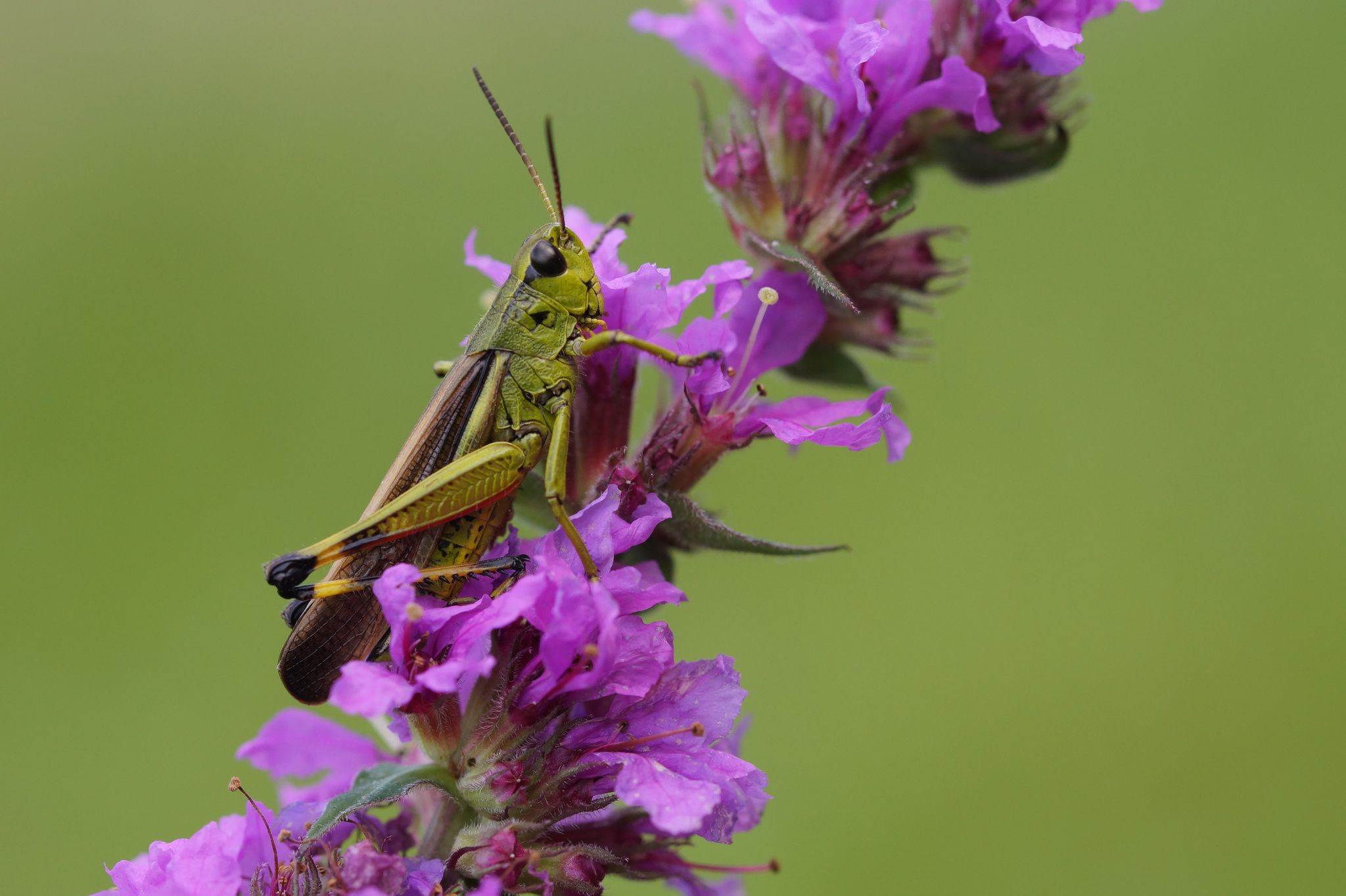
In Europe, four orders of arthropods perform the vast majority of pollination: Hymenoptera (bees and wasps), Diptera (flies), Lepidoptera (butterflies and moths), and Coleoptera (beetles)30. Further, there are four other taxa of arthropods that are more rarely seen on flowers and are not typically considered pollinators because they visit flowers so infrequently and/or deliver little pollen per visit31. These include the order Orthoptera (grasshoppers and leafhoppers), the order Hemiptera (true bugs), the order Araneae (spiders), and the family Formicidae (ants). Thus, it is necessary to consider the eight groups of arthropods to classify flower visitors as seen in Fig. 1.
In this study, we test whether a deep learning approach allows to localize and classify arthropods into these eight groups with sufficient accuracy. Therefore, we evaluated the performance of three light-weight object detection algorithms. The YOLO32 family of object detection algorithms offers multiple versions of its algorithm varying in a wide variety of use cases. In our experimental set-up, three different YOLO models were trained on more than 17,000 annotated images with the location of each arthropod being marked by bounding box coordinates. Using YOLO for object detection provides us with the benefit of detecting several arthropods in a single image, which is one of the reasons we want to explicitly test how well this task is performed. Additionally, we expected that one of the more difficult classifications will be of Dipterans in the family Syrphidae (hoverflies), which have mimicry of bees and wasps (Hymenoptera)33. Thus, we performed a separate test to see how well our model differentiates this family of flies from Hymenoptera on 1000 annotated images of hoverflies.

Example images for the eight groups in our dataset used for classification.
Methods
Dataset
The dataset covers the eight groups as seen in Fig. 1 and in Table 1: spiders (Araneae), beetles (Coleoptera), true flies (Diptera), true bugs (Hemiptera), bees and wasps (Hymenoptera), ants (Hymenoptera Formicidae), moths and butterflies (Lepidoptera), and crickets and grasshoppers (Orthoptera). Coleoptera, Diptera, Hymenoptera and Lepidoptera represent the most important pollinator groups of the dataset. These four orders make up the majority (aprox. 98%) of arthropods that visit flowers30. Ants (Hymenoptera in the family Formicidae) have been documented as pollinators in a few case studies, but have an insignificant role in pollination for most plants and can even be detrimental42. Likewise, Araneae, Hemiptera and Orthoptera might rarely be seen on flowers but will not play a significant role as pollinators, and can be detrimental as predators of pollinators43,44. Therefore, including these orders into the dataset prevents models from confusing them with the pollinator groups.
We used curated images indexed by the Global Biodiversity Information Facility (GBIF) database. A significant proportion of the images (96.77%) are sourced from the citizen science platforms, iNaturalist and Observation.org, which account for 53.86% and 42.91% of the contributions respectively. We extracted the occurrence data for our eight groups, and only kept the occurrence data that offered URLs with images. We then curated the datasets, focusing on species marked as present in Europe. For the orders Diptera, Coleoptera, Hymenoptera and Lepidoptera, we only sampled from known families of flower visitors. There was an uneven distribution of images across families within an order and across species within a family. For example, within the order Diptera, the Syrphidae family has many more images indexed by GBIF than other Dipteran families. Within the Syrphidae family, the common and widespread species Eristalis tenax is overrepresented compared to other species. Our methods therefore aimed to capture the taxonomic (and likely morphological) diversity of images that capture the representative range for each order, and to use random sampling in order to avoid selection biases. Specifically, for families consisting of more than 200 species, we randomly selected 200 species, and randomly choose one image per species. For families with fewer than 200 species, we randomly selected multiple images per species.
There is a high variability in the dataset with images of arthropods from different angles, exposure, focus, framing sizes and focal length. Also, there are various image backgrounds from artificial to natural ones. These characteristics are representative of those found in the iNaturalist dataset45. Images are captured using a variety of devices, from professional cameras to mobile phones. The citizen science platforms encourage users to crop their raw images such that arthropods appear more prominent. However, the degree to which this is applied varies among users, resulting in images where the arthropods occupy a significant portion of the image area in some cases, and a smaller portion in others. This introduces an inherent variability in the framing or ‘crop level’ of the insects across the dataset. The average area occupied by the insects, expressed as a proportion of the total image area (relative bounding box area), is 0.34 (Table 1), with an interquartile range between 0.10 and 0.54. Thus, our methods should allow for results that can be effectively extrapolated to further images captured by citizen scientists.
Each arthropod in these images was manually annotated with a bounding box by entomologists using the open source VIA Annotation program46. We discarded images that were identified incorrectly, showed larva and pupa stages, the arthropod was missing, and/or did not show the entire body of the arthropod. Our initial dataset consisted of 20,505 images of which we discarded 2,797 images. Table 1 shows the final sample sizes for training, validation, and testing. We split our dataset into a group-balanced validation and testing dataset. We used 210 images per group for testing and validation, and remaining images for training. The testing dataset was never shown to the object detection architecture, while the validation dataset was used for monitoring the model performance during the training procedure and for determining when to stop training in order to avoid overfitting.
YOLO
We assess the potential of three one-stage object detection models. We chose light-weight models with the intention that future applications will require the algorithms to run on mobile devices. Simultaneously, a trade-off must be made in which the detection model must be capable of performing successful classification tasks. YOLO32 is a one stage object detector, since it can integrate object classification and object location into one network architecture. The YOLO object detection algorithm divides the input image into SxS grids and each grid cell is responsible for predicting the object centered in that grids cell. Each grid cell predicts a number of bounding boxes and their corresponding confidence scores. Formally, confidence scores for each prediction are defined. This indicates the likelihood of objects and shows confidences of its prediction. At the same time, regardless of the number of boxes, conditional probabilities are predicted in each grid cell. It should be noted that only the contribution from the grid cell containing an object is calculated. While the original YOLO version was capable of real time detection, one of its biggest drawbacks was its performance on small objects. YOLOv247 introduced batch normalization, anchor points and the use of higher resolution images. YOLOv348 built upon previous models by adding an object score to bounding box prediction, added connections to the backbone network layers and made predictions at three separate levels of granularity to improve performance on smaller objects. YOLOv449 introduced further improvements in its backbone, feature aggregation, and its head for the detection step. Furthermore a set of data augmentation and activation functions could improve results.
YOLOv5
YOLOv550 was originally developed in PyTorch and not DarkNet like its predecessors. YOLOv5 offers multiple models, the difference between them is the trade-off between the size of the model and inference time. There are six different architectures specific to YOLOv5 (nano, small, medium, large and extra-large), they are distinguished from each other by the depth of the network, primarily the backbone network with the number of convolutional layers. In YOLOv5 the cross stage partial (CSP) networks are used as a backbone to extract features. In YOLOv5 PANet51 is used for the neck to get feature pyramids. The model head is mainly used to perform the final detection part. YOLOv5 applies anchor boxes on features and generates the final output vectors with probabilities, an objectness score, and bounding boxes. YOLOv5 authors decided to use a combination of Leaky ReLU and Sigmoid activation functions. In YOLOv5, the default optimization function for training is stochastic gradient descent (SGD) and the default loss function used is the binary cross entropy with logits.
YOLOv7
In YOLOv752 multiple incremental improvements were made from its previous versions. Extended efficient layer aggregation (E-ELAN) is used as a computational block, which enables quicker back-propagation and speeds up training and inference time. YOLOv7 scales the network depth and width while concatenating layers together. Reparameterization techniques, which involve averaging a set of model weights, creates models that are more robust in learning patterns. The YOLOv7 authors use gradient flow propagation paths to see which modules in the network should use reparameterization strategies and which should not. For the final predictions the authors use an auxiliary head with different levels of supervision, settling on a coarse to fine definition where supervision is passed back from the lead head at different granularities.
Training set-up
We selected three models YOLOv5n (nano), YOLOv5s (small), and YOLOv7t (tiny) to compare to each other. All three models offer less than ten million trainable parameters and are capable for real time detection even on CPUs and low end hardware GPUs. The models were trained using an input image size of 640*640 pixels in order to use a batch size of eight for all models, which was the highest value allowed by the available hardware. We decided not to train the models from scratch, but to use pre-trained weights from the COCO53 dataset which are provided with each YOLO repository, since this can result in more robustness in the model performance54. All models are trained using three epochs to “warmup” the optimizer, since this can help with faster convergence55 and with the same set of hyper-parameters for 300 epochs (See supplementary information Table 1), while the best model is determined by its fitness using a weighted average of the mean average precision at various intersection over union thresholds. To evaluate our models we used the following metrics: overall accuracy, precision, recall, intersection over union (IoU), and the false positive rate. The confusion matrix is formed to calculate group specific metrics. All three models provide a prediction confidence level and an IoU score threshold. Using the findings for the overall accuracy, the best possible combination was identified using a grid search from 10% to 90% in 10% increments for both thresholds (See Figs. 1–4 supplementary information). We report the accuracies depending on the highest overall accuracies achieved by the threshold grid search. The computations for this work were done using resources from the Leipzig University Computing Center which granted us quota access to compute nodes with eight Nvidia RTX2080Ti 11 GB each.
Results
We discovered that, in general, all three models (YOLOv5n, YOLOv5s, and YOLOv7t) were able to distinguish the order of flower visitors in images with high accuracies of up to 96 percent. As a result, we show that this method of categorization is capable of both finding the location of an arthropod within a picture and identifying it to its group.
For YOLOv5n the highest overall accuracy acheived 94.50%; this was achieved with a combination of a 20% confidence and 50% IoU threshold. YOLOv5s achieved 96.24% accuracy with a combination of a 30% confidence and 60% IoU threshold. YOLOv7t achieved 95.08% accuracy with a combination of 10% confidence and 30% IoU threshold. Despite their modest model sizes of less than 10 million trainable parameters, all models, YOLOv5n, YOLOv5s, and YOLOv7t, were able to recognize the order of flower visitors in images. YOLOv5s is approximately 3.8 times larger than YOLOv5n and achieves a 1.7% greater overall accuracy. YOLOv5s and YOLOv7t are nearly the same size and have an overall accuracy difference of less than 1.2%. The remaining accuracy metrics are shown in Table 2. Precision indicates how accurate predictions are, whereas recall measures the proportion of ground truth instances that were correctly identified by the model. The false positive rate (FPR) is the proportion of negative cases in data that were incorrectly recorded as positive. Note that YOLOv5n and YOLOv7t get comparable results, with the exception of the higher recall score for YOLOv7t. The IoU is determined for all true positives by taking the mean of all predicted bounding boxes in an image. All YOLO versions scored a mean IoU of above 78%.

Confusion matrix for all three models (a) YOLOv5n, (b) YOLOv5s, and (c) YOLOv7t. Columns show the predicted values and rows the actual label values.
The confusion matrix of the predictions on the test dataset for each of the three models is shown in Fig. 2. The matrix shows the eight groups in our dataset, in addition a background group (Bg.) is added to count false positives and false negatives as well. We show the confusion matrix using the confidence and Iou threshold from Table 2 scoring the highest overall accuracy. The confusion matrix visualizes and summarizes the classification of the algorithm’s performance, with each row of the matrix representing examples in an actual group and each column representing occurrences in a predicted group. Since there may be many label bounding boxes for a given picture, the total number of images in a row may exceed 210 even if each row contains exactly 210 images from the test dataset in Table 1. All three YOLO models in Fig. 2, YOLOv5n (Fig. 2a), YOLOv5s (Fig. 2b), and YOLOv7t (Fig. 2c), exhibit similar behavior, with the diagonal indicating true positive scores always greater than 75%. It is worth noting that all three models had some missed detections for the Hemiptera and Hymenoptera Formicidae groups. As seen in Table 1 this can be linked to small bounding boxes and several overlapping labels per picture. Both groups share noticeable smaller bounding boxes as well as a higher ratio of bounding boxes per image compared to other groups. As shown in the first row of the confusion matrix in Fig. 2c, YOLOv7t suffers from more false positives than its YOLOv5 counterparts.

The figures show results for YOLOv7t, (a) IoU depending on the number of bounding boxes per images [nBB], (b) IoU depending on the relative area of the bounding box to the image size [BBarea], and (c) counts of the number of bounding boxes in our dataset for each combined category of nBB and BBarea. The size and color of each dot represents the number of bounding boxes.
Aside from comparing metrics between YOLO versions, we also look closely at outcomes for detecting several objects in a single image and images with small bounding box labels as seen in Fig. 3. The ability to recognize many arthropods of various types in a single image is a significant advantage of employing object detection rather than scene classification approaches. In these challenging situations, we particularly examine the IoU metric as the accuracy of the bounding box placement as a very relevant indicator of the models performance. The results on images grouped by their number of labels per image is shown in Fig. 3a, and the results for predictions depending on the relative area of its bounding box in Fig. 3b. In Fig. 3a the IoU score is shown for images with the number of detections ranging from one to ten, while the last group consists of all images with more than ten detections. In Fig. 3b the IoU score is shown depending on the relative area of the bounding box in relations to its image size, the higher the value of BBarea the larger is the bounding box. The IoU measurements demonstrate a significant drop in their values when the number of labels per image increase. The same effect can be observed when dealing with small bounding boxes. In Fig. 3c we compare the number of bounding boxes per images and the relative area of the bounding boxes is shown. We can see that a larger number of bounding boxes on images also corresponds to a lower relative bounding box size, while larger bounding box areas are typically found on images where there is only one single bounding box. It is also worth noting that in Fig. 3b,c the group Hymenoptera Formicidae are responsible for the bulk of the smaller bounding boxes, and as a result, they have a considerable influence on the distribution of bounding boxes. This is especially noticeable in Fig. 3c, where the large circle in the upper left corner highlights the impact.
We carried out an additional test in which we compared the detection results of the family Syrphidae within Diptera using the YOLOv7t model. Table 3 shows accuracy metrics for two combinations of confidence and IoU thresholds, where the first, using 10% confidence & 30% IoU was used due to scoring the highest overall accuracy from Table 2 and the second combination of 30% confidence & 60% IoU, which scores the highest overall accuracy for the Syrphidae dataset (See supplementary information Fig. 5). While both experiments demonstrated exceptional results, it can be argued that using 30% confidence & 60% IoU was slightly superior, as it exhibited a higher level of overall accuracy, precision, and false positive rate, however, both experiments should be deemed highly successful as they both correctly classified Syrphidae. Table 4 shows the confusion matrix for threshold combination of 30% confidence & 60% IoU. The confusion matrix is computed using the 1061 images of Syrphidae, to test whether the YOLOv7t model misclassifies the family into different groups, specifically the Hymenoptera order that they mimic. From Table 4 we can see that of the 1061 Syrphidae, only 55 are classified as Hymenoptera, which is the highest amount of the misclassified detections, as well as 39 labels of bounding box which were not recognized at all. Successful classification examples can be seen in Fig. 4d,f.

Predictions (blue) and labels (red) for nine images of arthropods in our dataset using the YOLOv7t model.
In Fig. 4 some of the predictions made by the YOLOv7t model are depicted, including predictions of images with multiple arthropods. The figure shows nine images of seven orders from our dataset. While the YOLOv7t model correctly classifies all arthropods to its specific group, in cases with a large count of small labels there are some false negatives as seen in Fig. 4e,g,h. Figure 4c,d,f shows that the YOLOv7t correctly differentiates between Diptera-Syrphidae and Hymenoptera.
Discussion
Identifying flower-visiting arthropods is a challenging task, especially when one considers the trade-off that must be made between the amount of processing power necessary and the degree of accuracy that must be achieved in order to get acceptable results. The YOLO versions used in this study, v5 and v7, provide several options for models that would be suited to this problem. We tested three light-weight models that could be deployed in a field setting for automated pollinator monitoring: YOLOv5 with the smallest sizes, “nano” (n) and “small” (s), and YOLOv7 with the smallest size, “tiny” (t). We have found that the results of YOLOv5s and YOLOv7t are quite similar. The parameter counts of YOLOv5s and YOLOv7t are very comparable. YOLOv5n, on the other hand, has a much reduced size and this likely explains its lower scores as we found that the number of parameters influenced all of the accuracy metrics.
The advantage of using object detection rather than scene classification is not only in determining the location of the arthropod on the photos, but also in recognizing several arthropods in one image. This is important for the development of future automated pipelines for pollinator monitoring because it allows all individuals visiting a flower to be counted and identified. However, we observed that the model performance drops slightly when there are multiple arthropods in an image (Fig. 3). This is because models are faced with the challenge of small objects, since images with multiple arthropods typically contain smaller bounding boxes than images of a single arthropod. When there is only one arthropod to locate in the image, both YOLOv5s and YOLOv7t give similar results.
The high accuracy of the model in distinguishing the Syrphidae from Hymenoptera demonstrates the potential of the model to be a reliable tool. It is a relatively easy job to distinguish between some of the morphologically distinct groups in our study, such as Lepidoptera and Coleoptera. However, distinguishing Dipterans in the family Syrphidae from Hymenopterans is a challenging task, as Syrphidae mimic the morphological appearance of bees and wasps in the order Hymenoptera65. The high performance of our model in this task suggests great promise for future development of models, which will aim to classify each image to the lowest taxonomic level that an expert could with high accuracy.
A major challenge in understanding trends and drivers in pollinators and pollination is insufficient monitoring, as our current data is geographically biased and uses inconsistent methodology. Mobilizing citizen scientists is one solution that works well for charismatic taxa that are easy to identify, such as butterflies. Indeed, more than 3000 transects are monitored for butterflies each year by citizens throughout Europe66,67. However, expanding such monitoring to other pollinating taxa is difficult, as most citizens are not interested in learning to distinguish amongst Dipteran families or in killing the arthropods they observe so that they can be identified by experts. The results presented here are working towards a future in which pollinators and plant-pollination interactions are consistently and non-destructively monitored across broad spatio-temporal scales using time-lapse cameras set to photograph flowers in the field and then using CNNs to classify arthropods in those images. In Europe, such monitoring schemes could be possible in existing distributed networks such as the European Long Term Ecosystem Research (eLTER) network. However, it is an open question how well our CNN models developed in this manuscript, which use GBIF-indexed images, will perform on classifying images that are collected by a time-lapse camera. Testing how well our models perform on such an out-of-sample dataset is an important direction for future research.
Object detection algorithms using deep learning have proven to be effective in achieving high accuracy in a variety of tasks, making them a popular choice for machine learning practitioners. However, the complexity and computational requirements of incredible deep networks can make it challenging to deploy them in real-world applications where resources may be limited or the need for quick decision-making is crucial. Given this, it’s important to consider deep learning models using fewer trainable parameters that may not have the same level of accuracy but are more practical for deployment in the real world. While deeper networks still hold potential for improving accuracy, it may be necessary to balance that with considerations of practicality and feasibility in real-world settings.
Our study represents a significant advancement in the field of AI-assisted identification of European flower visitors, as we encompass a wide range of arthropod taxa in our training data set that occur on a wide variety of floral backgrounds (and other complex backgrounds). However, we see this as an initial step in the progress that is needed for automated insect identification, as many ecological questions and monitoring aims will require identification at lower taxonomic levels. Entomologists that specialize in taxonomy would hypothesize that species-level identification might not be possible, as identifying features at the species level are not visible on field images, such as features of the genitalia, placement of hairs on the legs, etc. However, traditional convolutional neural networks (CNNs) have the potential to surpass human-level classification in detecting pollinators by identifying intricate features and patterns that may elude the human eye68. Thus, we see testing the potential and limits of CNNs for family, genera, and species level identification of insect pollinators as an exciting next step in this line of research.
Conclusion
In the near future, object detection will be a vital component of pollinator monitoring, allowing ecologists to have near real time data on pollination across broad spatial gradients. To correctly evaluate changes in plant-pollinator interactions across space and time, it will be essential that we continue to develop this technology, as well as data sets that can be utilized for training models. We have shown that the YOLO object detection models can be used to classify arthropod orders and localize the arthropods with bounding boxes. Localization is an important task to consider for the development of AI applications in pollination ecology because quantifying plant-pollinator networks requires also abundance information (counts of individual arthropods). We chose to evaluate three different light YOLO models: YOLOv5-nano, YOLOv5-small, and YOLOv7-tiny, which all have less than ten million trainable parameters. This is important for the future development of edge AI applications in pollination ecology because lighter models can be deployed to run detection in real time on edge devices under field conditions, with limited computational power and limited energy supply. The YOLOv5-nano model was selected for use as the foundation because it provides the lowest number of parameters while still delivering a satisfactory compromise between precision and speed. YOLOv5-small and YOLOv7-tiny models share similar number of parameters and, therefore do not differ much in their results. The results scale almost linearly with the number of parameters. Therefore, a suitable model type can be selected from our tests depending on the capabilities of future low-cost hardware setup to monitor pollination.
Data availability
The datasets generated during and/or analyzed during the current study are available from the corresponding author on reasonable request. The scripts to run all experiments are publicly available through our GitHub page stark-t/PAI.
References
Ollerton, J., Winfree, R. & Tarrant, S. How many flowering plants are pollinated by animals?. Oikos 120, 321–326 (2011).
Potts, S. G. et al. The assessment report of the intergovernmental science-policy platform on biodiversity and ecosystem services on pollinators, pollination and food production. In Intergovernmental Science-Policy Platform on Biodiversity and Ecosystem Services (2016).
Bennett, J. M. et al. A review of European studies on pollination networks and pollen limitation, and a case study designed to fill in a gap. AoB Plants 10, ply068 (2018).
Creedy, T. J. et al. A validated workflow for rapid taxonomic assignment and monitoring of a national fauna of bees (apiformes) using high throughput DNA barcoding. Mol. Ecol. Resour. 20, 40–53. https://doi.org/10.1111/1755-0998.13056 (2020).
Jarić, I. et al. iEcology: harnessing large online resources to generate ecological insights. Trends Ecol. Evol. 35, 630–639 (2020).
Spiesman, B. J. et al. Assessing the potential for deep learning and computer vision to identify bumble bee species from images. Sci. Rep. 11, 1–10 (2021).
Weinstein, B. G. A computer vision for animal ecology. J. Anim. Ecol. 87, 533–545 (2018).
Wäldchen, J. & Mäder, P. Machine learning for image based species identification. Methods Ecol. Evol. 9, 2216–2225 (2018).
Goëau, H., Bonnet, P. & Joly, A. Overview of lifeclef plant identification task 2019: diving into data deficient tropical countries. In CLEF 2019-Conference and Labs of the Evaluation Forum, vol. 2380, 1–13 (CEUR, 2019).
Júnior, T. D. C. & Rieder, R. Automatic identification of insects from digital images: A survey. Comput. Electron. Agric. 178, 105784 (2020).
Høye, T. T. et al. Deep learning and computer vision will transform entomology. Proc. Natl. Acad. Sci. 118, e2002545117 (2021).
Ratnayake, M. N., Dyer, A. G. & Dorin, A. Tracking individual honeybees among wildflower clusters with computer vision-facilitated pollinator monitoring. PLoS ONE 16, e0239504 (2021).
Litjens, G. et al. A survey on deep learning in medical image analysis. Med. Image Anal. 42, 60–88. https://doi.org/10.1016/j.media.2017.07.005 (2017).
Ronneberger, O., Fischer, P. & Brox, T. U-net: Convolutional networks for biomedical image segmentation. In Medical Image Computing and Computer-Assisted Intervention–MICCAI 2015 (eds Navab, N. et al.) 234–241 (Springer, 2015).
Wurm, M., Stark, T., Zhu, X. X., Weigand, M. & Taubenböck, H. Semantic segmentation of slums in satellite images using transfer learning on fully convolutional neural networks. ISPRS J. Photogramm. Remote. Sens. 150, 59–69 (2019).
Stark, T., Wurm, M., Zhu, X. X. & Taubenböck, H. Satellite-based mapping of urban poverty with transfer-learned slum morphologies. IEEE J. Sel. Top. Appl. Earth Obs. Remote Sens. 13, 5251–5263 (2020).
Zhu, X. X. et al. Deep learning in remote sensing: A comprehensive review and list of resources. IEEE Geosci. Remote Sens. Mag. 5, 8–36 (2017).
van Klink, R. et al. Emerging technologies revolutionise insect ecology and monitoring. Trends Ecol. Evol. 37, 872–885. https://doi.org/10.1016/j.tree.2022.06.001 (2022).
Buschbacher, K., Ahrens, D., Espeland, M. & Steinhage, V. Image-based species identification of wild bees using convolutional neural networks. Ecol. Inform. 55, 101017 (2020).
Kaya, Y., Kayci, L. & Uyar, M. Automatic identification of butterfly species based on local binary patterns and artificial neural network. Appl. Soft Comput. 28, 132–137 (2015).
Almryad, A. S. & Kutucu, H. Automatic identification for field butterflies by convolutional neural networks. Eng. Sci. Technol. Int. J. 23, 189–195 (2020).
Mielczarek, ŁE. & Tofilski, A. Semiautomated identification of a large number of hoverfly (Diptera: Syrphidae) species based on wing measurements. Orient. Insects 52, 245–258 (2018).
Abeywardhana, D., Dangalle, C., Nugaliyadde, A. & Mallawarachchi, Y. Deep learning approach to classify tiger beetles of Sri Lanka. Ecol. Inform. 62, 101286 (2021).
Cao, X., Wei, Z., Gao, Y. & Huo, Y. Recognition of common insect in field based on deep learning. In Journal of Physics: Conference Series, vol. 1634.
Bjerge, K. et al. Accurate detection and identification of insects from camera trap images with deep learning. PLoS Sustain. Transform. 2, e0000051 (2023).
Ratnayake, M. N., Amarathunga, D. C., Zaman, A., Dyer, A. G. & Dorin, A. Spatial monitoring and insect behavioural analysis using computer vision for precision pollination. Int. J. Comput. Vis. 131, 591–606 (2023).
Droissart, V. et al. Pict: A low-cost, modular, open-source camera trap system to study plant-insect interactions. Methods Ecol. Evol. 12, 1389–1396 (2021).
Naqvi, Q., Wolff, P. J., Molano-Flores, B. & Sperry, J. H. Camera traps are an effective tool for monitoring insect–plant interactions. Ecol. Evol. 12, e8962 (2022).
Sittinger, M. Insect Detect—Software for automated insect monitoring with a DIY camera trap system. If you use this software, please cite it as below. https://doi.org/10.5281/zenodo.7793296 (2023).
Wardhaugh, C. W. How many species of arthropods visit flowers?. Arthropod-Plant Interact. 9, 547–565 (2015).
Herrera, C. M. Components of pollinator” quality”: Comparative analysis of a diverse insect assemblage. Oikos 79–90 (1987).
Redmon, J., Divvala, S., Girshick, R. & Farhadi, A. You only look once: Unified, real-time object detection. In Proceedings of the IEEE conference on computer vision and pattern recognition, 779–788 (2016).
Leavey, A., Taylor, C. H., Symonds, M. R. E., Gilbert, F. & Reader, T. Mapping the evolution of accurate Batesian mimicry of social wasps in hoverflies. Evolution 75, 2802–2815. https://doi.org/10.1111/evo.14336 (2021).
Dmitry. https://inaturalist-open-data.s3.amazonaws.com/photos/75694598/original.jpeg (2023). [Online; Accessed 08 March 2023].
Rayego, J. M. P. https://inaturalist-open-data.s3.amazonaws.com/photos/137238652/original.jpg (2023). [Online; Accessed 08 March 2023].
https://observation.org/photos/1350015.jpg (2023). [Online; Accessed 08 March 2023].
Février, J. https://inaturalist-open-data.s3.amazonaws.com/photos/97183178/original.jpeg (2023). [Online; Accessed 08 March 2023].
Daniels, S. https://inaturalist-open-data.s3.amazonaws.com/photos/9517541/original.jpeg (2023). [Online; Accessed 08 March 2023].
https://observation.org/photos/17292380.jpg (2023). [Online; Accessed 08 March 2023].
Gorosti, S. https://observation.org/photos/19056353.jpg (2023). [Online; Accessed 08 March 2023].
Gabler, P. https://inaturalist-open-data.s3.amazonaws.com/photos/61786141/original.jpg?1582137611 (2023). [Online; Accessed 08 March 2023].
Rico-Gray, V. & Oliveira, P. S. The Ecology and Evolution of Ant–Plant Interactions (University of Chicago Press, 2007).
Suttle, K. B. Pollinators as mediators of top–down effects on plants. Ecol. Lett. 6, 688–694. https://doi.org/10.1046/j.1461-0248.2003.00490.x (2003).
Knight, T. M., McCoy, M. W., Chase, J. M., McCoy, K. A. & Holt, R. D. Trophic cascades across ecosystems. Nature 437, 880–883 (2005).
Van Horn, G. et al. The inaturalist species classification and detection dataset. In Proceedings of the IEEE conference on computer vision and pattern recognition, 8769–8778 (2018).
Dutta, A. & Zisserman, A. The via annotation software for images, audio and video. In Proceedings of the 27th ACM International Conference on Multimedia, MM ’19, 2276–2279 (Association for Computing Machinery, 2019). https://doi.org/10.1145/3343031.3350535.
Redmon, J. & Farhadi, A. Yolo9000: Better, faster, stronger. In Proceedings of the IEEE Conference on Computer Vision and Pattern Recognition, 7263–7271 (2017).
Redmon, J. & Farhadi, A. Yolov3: An incremental improvement. arXiv preprint arXiv:1804.02767 (2018).
Bochkovskiy, A., Wang, C.-Y. & Liao, H.-Y. M. Yolov4: Optimal speed and accuracy of object detection. arXiv preprint arXiv:2004.10934 (2020).
Jocher, G. ultralytics/yolov5: v3.1—Bug Fixes and Performance Improvements. https://github.com/ultralytics/yolov5, https://doi.org/10.5281/zenodo.4154370 (2020).
Liu, S., Qi, L., Qin, H., Shi, J. & Jia, J. Path Aggregation Network for Instance Segmentationhttps://doi.org/10.48550/ARXIV.1803.01534 (2018).
Wang, C.-Y., Bochkovskiy, A. & Liao, H.-Y. M. Yolov7: Trainable bag-of-freebies sets new state-of-the-art for real-time object detectors. arXiv preprint arXiv:2207.02696 (2022).
Lin, T.-Y. et al. Microsoft coco: Common objects in context. In European Conference on Computer Vision, 740–755 (Springer, 2014).
Hendrycks, D., Lee, K. & Mazeika, M. Using pre-training can improve model robustness and uncertainty. In International Conference on Machine Learning, 2712–2721 (PMLR, 2019).
Goyal, P. et al. Accurate, large minibatch sgd: Training imagenet in 1 hour. arXiv preprint arXiv:1706.02677 (2017).
Halinaa. https://inaturalist-open-data.s3.amazonaws.com/photos/112626710/original.jpeg (2023). [Online; Accessed 08 March 2023].
https://inaturalist-open-data.s3.amazonaws.com/photos/7514692/original.jpeg (2023). [Online; Accessed 08 March 2023].
Consolo, M. https://inaturalist-open-data.s3.amazonaws.com/photos/1919537/original.jpg?1444411952 (2023). [Online; Accessed 08 March 2023].
https://observation.org/photos/8301252.jpg (2023). [Online; Accessed 08 March 2023].
Alexis. https://inaturalist-open-data.s3.amazonaws.com/photos/76067599/original.jpeg (2023). [Online; Accessed 08 March 2023].
https://observation.org/photos/21035810.jpg (2023). [Online; Accessed 08 March 2023].
Pecoraro, M. https://inaturalist-open-data.s3.amazonaws.com/photos/119665574/original.jpeg (2023). [Online; Accessed 08 March 2023].
Poessé, D. https://observation.org/photos/4893356.jpg (2023). [Online; Accessed 08 March 2023].
Herr, C. https://inaturalist-open-data.s3.amazonaws.com/photos/150082853/original.jpeg?1628698986 (2023). [Online; Accessed 08 March 2023].
Penney, H. D., Hassall, C., Skevington, J. H., Lamborn, B. & Sherratt, T. N. The relationship between morphological and behavioral mimicry in hover flies (Diptera: Syrphidae). Am. Nat. 183, 281–289 (2014).
Van Swaay, C. A. et al. The EU butterfly indicator for grassland species: 1990–2017. technical report. Technical Report (2019).
Europe, B. C. & the Centre for Ecology & Hydrology. Butterfly-monitoring (2023).
He, K., Zhang, X., Ren, S. & Sun, J. Delving deep into rectifiers: Surpassing human-level performance on imagenet classification. In Proceedings of the IEEE International Conference on Computer Vision, 1026–1034 (2015).
Acknowledgements
This research was funded by the Helmholtz AI initiative (Information & Data Science) Pollination Artificial Intelligence (ZT-I-PF-5-115), lead by Prof. Tiffany M. Knight and Prof. Hannes Taubenboeck.
Funding
Open Access funding enabled and organized by Projekt DEAL.
Author information
Authors and Affiliations
Contributions
T.S., V.S., M.W., H.T., T.M.K. designed the scope of the study. V.S. and T.M.K. were responsible for the creation of the dataset, T.S., V.S., and R.S. were responsible for methods and experiments. T.S. took the lead in writing the manuscript with significant contributions of V.S and T.M.K.. M.W. H.T., and T.M.K. reviewed the manuscript.
Corresponding author
Ethics declarations
Competing interests
The authors declare no competing interests.
Additional information
Publisher's note
Springer Nature remains neutral with regard to jurisdictional claims in published maps and institutional affiliations.
Supplementary Information
Rights and permissions
Open Access This article is licensed under a Creative Commons Attribution 4.0 International License, which permits use, sharing, adaptation, distribution and reproduction in any medium or format, as long as you give appropriate credit to the original author(s) and the source, provide a link to the Creative Commons licence, and indicate if changes were made. The images or other third party material in this article are included in the article's Creative Commons licence, unless indicated otherwise in a credit line to the material. If material is not included in the article's Creative Commons licence and your intended use is not permitted by statutory regulation or exceeds the permitted use, you will need to obtain permission directly from the copyright holder. To view a copy of this licence, visit http://creativecommons.org/licenses/by/4.0/.
About this article

Cite this article
Stark, T., Ştefan, V., Wurm, M. et al. YOLO object detection models can locate and classify broad groups of flower-visiting arthropods in images. Sci Rep 13, 16364 (2023). https://doi.org/10.1038/s41598-023-43482-3
Received:
Accepted:
Published:
DOI: https://doi.org/10.1038/s41598-023-43482-3
Comments
By submitting a comment you agree to abide by our Terms and Community Guidelines. If you find something abusive or that does not comply with our terms or guidelines please flag it as inappropriate.
