
Abstract
Automatic diagnosis of malignant prostate cancer patients from mpMRI has been studied heavily in the past years. Model interpretation and domain drift have been the main road blocks for clinical utilization. As an extension from our previous work we trained on a public cohort with 201 patients and the cropped 2.5D slices of the prostate glands were used as the input, and the optimal model were searched in the model space using autoKeras. As an innovative move, peripheral zone (PZ) and central gland (CG) were trained and tested separately, the PZ detector and CG detector were demonstrated effective in highlighting the most suspicious slices out of a sequence, hopefully to greatly ease the workload for the physicians.
Introduction
In this section, the literature in the field of diagnosis of prostate cancer (PCa) from medical images, the current state-of-the-art research of using deep learning algorithms in automating the diagnosis process and challenges in closing the gap of research and clinical utilization is discussed.
Background
Prostate cancer (PCa) has been studied for its commonality and high mortality rate in the United States. As recommended by almost all the cancer types, early detection through regular screening plays an essential role in reducing the mortality rate and improving quality of life for PCa patients (https://www.cancer.org/cancer/prostate-cancer/about/key-statistics.html). In clinics, the diagnosis is made based on the screenings and the biopsies. To be specific, the biopsy serves as the golden standard when it comes to determining the malignancy of a suspicious lesion. However, the procedure of a typical prostate biopsy is invasive and complications such as hemorrhage, dysuria and infections have been reported. Cases of disagreement between the biopsy and the screenings have been reported though rarely1.
Among the screening techniques, multiparametric magnetic resonance imaging (mpMRI) has shown increasing impact in clinical decision making. Popular sequences include T2-weighted (T2W), diffusion-weighted imaging (DWI), dynamic contrast-enhanced imaging (DCE) and MR spectroscopy. According to the report, best visual of PCa lesions happens when the sequences are integrated in a parametric format2,3.
The definition of malignancy in the clinics correlates to Gleason score 7 (including 3 + 4) in histopathology4 and automatic detection of which from the mpMRI is the goal of this work. To be specific, the techniques used in automating the screen reading process are machine learning and computer vision customized in this particular tasks5.
For the past few years, deep learning models have made progress in making diagnosis from reading chest X-ray6, mammogram7, and mpMRI8,9.
However, small sample size has been one of the challenges for deep machine learning algorithms to learn a good pattern from limited data and labelling. Data acquisition and sharing is a process that is concerning policy and regulations, with patients’ privacy and medical ethics put forward. Data labelling on the patient level is labor-intensive and also restricted with the regulations. While data collection is under the way for many institutions, efforts have been made to leverage from sophisticated models trained on large-scale data sets consisting of natural images10,11,12.
Previous work
Data used in the study was originated from the SPIE-AAPM-NCI Prostate MR Gleason Grade Group Challenge13, which aimed to develop quantitative mpMRI biomarkers for determination of malignant lesions in PCa patients. PCa patients were previously de-identified by SPIE-AAPM-NCI and The Cancer Imaging Archive (TCIA).

Sample images of the cropped 64 × 64 pixel rectangle from all four modalities: T2, ADC, DWI, and K-trans after resampling and registration. The lesions are malignant in PZ, benign in PZ, malignant in CG, and benign in CG from row 1 to 4 respectively.
Each patient came with four modalities displayed as in Fig. 1. Lesions exhibited hypointense signals in T2 weighted and apparent diffusion coefficient (ADC) map, and hyperintense signals in diffusion weighted imaging with low b values (b = 50). The modality of k-trans was not included in the input channels for failing to visually differentiate cancer and disease under k-trans.
In our previous work, we found that multi-modality input contributed significantly to accurate classification. In most cases, class activation map (CAM)14 helped provide the proof about where the model is looking at when making predictions. The central point of the potential lesion was provided13.
One step closer to clinical utilization by easing the workload of a medical expert is the focus and contribution of this paper. Contributions of this paper can be summarized as the following. (1) We inputted into the classification models the entire prostate gland (PZ and CG separately) rather than the cropped region of interest (ROI). (2) According to Fig. 1, lesion can exhibit very different characteristics when residing in PZ and CG. Another attempt in improving upon our previous work was to train and test using separate models for PZ and CG. (3) To verify the robustness of the trained model, we tested it on an independent cohort from our own institute . Experimental results showed that the trained PZ-detector and CG-detector were able to rank the probability of malignancy for each slice and highlight the suspicious slices out of the sequence, despite of the challenges that the testing samples are generated from different scanners with different parameters.
Data
In this section, imaging acquisition parameters and image pre-processing steps are described in detail.
Scanning parameters
The images were acquired on two different types of Siemens 3T MR scanners, the MAGNETOM Trio and Skyra. T2W images were acquired using a turbo spin echo sequence and had a resolution of around 0.5 mm in plane and a slice thickness of 3.6 mm. The DWI series were acquired with a single-shot echo planar imaging sequence with a resolution of 2 mm in-plane and 3.6 mm slice thickness and with diffusion-encoding gradients in three directions. Three b-values were acquired (50, 400, and 800 s/mm2), and subsequently, an ADC map was calculated by the scanner software.
To test cross-institutional generalization capability of our model, an independent cohort (test cohort 2) consisting of 40 patients was collected for testing from our own institution with the IRB-approval. An ultrasound-guided needle biopsy was performed to confirm the diagnosis. Two image modalities were acquired for each patient using a 3.0 T MR scanner (Ingenia, Philips Medical System, the Netherlands) using small field of view as follows: T2W acquired with Fast-Spin-Echo (TE/TR: 4389/110ms, Flip Angle: 90° with image resolution of 0.42 × 0.42 × 2.4mm3) and DWI with two b values (0 and 1000 s/mm2). The voxel-wise ADC map was constructed using these two DWIs.
Data pre-processing
All images were resampled and registered to T2-axial image sets in the software of MIM (https://www.mimsoftware.com). N4 bias-field correction was applied to T2 and ADC for intensity uniformity correction. Then sub-regions such as PZ or CG were cropped from the sequence based on the contouring performed by our team of medical experts. Pre-processing and cropping on one slice were shown in Fig. 2. Gaussian blurring was applied to increase the contrast. Four extreme points were located based on the annotated contour. With a margin of 5 pixels, a surrounding rectangle was cropped.

PZ cropping steps on one slice of the sequence. Gaussian blurring was applied to increase the contrast. Four extreme points were located based on the annotated contour. With a margin of 5 pixels, a surrounding rectangle was cropped. CG cropping follows similar steps.
In the model training and inference stage, labelling is associated with the sequence rather than one slice. Therefore, the extreme points were searched through the sequence to not to miss any part of the PZ or CG, as shown in Figs. 3 and 4. The cropped sequence of sub-region of PZ or CG were then used as the input to train the PZ-detector and CG-detector, respectively. There are four patients with lesions spreading both PZ and CG. In these four cases, lesions were assigned to the sub-region based on the volumetric ratio from the bare eyes. In the experiment, as stated in the manuscript, we left a margin of 5 pixels when cropping the sub-region, which should leave enough room for including the lesion as an entirety.

PZ cropping results on one sequence consisting of 8 slices.

Example of cropped sub-regions with three consecutive slices. (left) PZ with Gleason Grade Group 3. (right) CG with Gleason Grade Group 2. (Upper) T2W. (Lower) ADC.
Method and results
Auto-keras
Auto deep learning models for medical image analysis have not been studied much. To fully take advantage of this technique, implementation details were illustrated as follows. Codings can be found at (https://github.com/WeiweiZongHFHS).
To increase the sample size, and to leverage the 3D information between two consecutive slices, the 2-channel input was augmented to include T2-ADC pair, consecutive T2 pairs and consecutive ADC pairs. Performance of using just T2-ADC pair and the mixed pairs were compared for both PZ and CG detectors.
The number of benign lesions outnumbered malignant lesions and re-weighting was used accordingly. After shuffling the data, one third of the public data were randomly selected for validation. The trained model was then tested on the test cohort 2.
Early stopping with a patience value of 10 and optimization goal of area-under-the-curve (AUC) for validation set was used to prevent overfitting. Bayesian tuner was used as the searching strategy and maximum searching epochs were set as 20. Bayesian tuner, as opposed to the regular greedy tuner, follows an iterative process rather than searching for every possible combination of parameters. At first, a few sets of parameters were selected at random. The next set of parameters was chosen based on the performance until reaching the pre-defined performance bar or the maximum iterations. Auto-augmentation included a search in the augmentation space with operations such as random flip, translation, and contrast, etc.
The learned optimal models to detect lesions in PZ and CG were displayed in Fig. 5. Compared to PZ-detector, data augmentation and network architecture were found more complicated to recognize malignant lesions in CG. However, the best validation AUC of 0.94 was achieved for CG-detector when only T2-ADC pairs were used as the input. According to Fig. 1, lesions in CG are visually difficult to detect from single source of modality, which might have explained the preference of T2-ADC pair as the input. The best validation AUC for PZ-detector, on the other hand, was 0.90, when the input was a mixture type of pairs.

Customized models with layer type, output shape and number of parameters for each layer to detect lesions in PZ (Upper) and CG (Lower), respectively.
In Fig. 6, gradient class activation map (Grad-CAM) was used to visualize the learned PZ-detector and CG-detector. The prediction probability was the value of the output node. It can be observed from the two cases that, lesions aligned well with the hyper-intense signal in the Grad-CAM if predicted malignant, otherwise neither hyper- nor hypo-intense signal was visible.

Grad-cam for PZ (left) and CG (right) respectively, showing the attention of the model aligned well with the lesion if malignant.
Challenges of domain drift
Testing data cohort was collected from our institute and posed several challenges during the inference stage.
-
(1)
Contours of PZ or CG were not available on contrary to the cases in the training cohort, but more of a realistic setting.
-
(2)
The ADC maps were calculated from DWI \(b = 0\) and \(b = 1000\). They are visually slightly different from the ADC maps in the training cohort.
-
(3)
Number of slices were varied in the testing cohort.
Solutions
-
(1)
We nevertheless tested PZ-detector and CG-detector on the testing cohort, where the input is the T2-ADC pair and whole prostate gland was used as the input since sub-region contour was not available. The PZ-detector was able to accurately highlight slices with suspicious malignant lesions. While the CG-detector was able to detect lesions in CG most of the time but were found prone to the false positive traps as shown in Fig. 7, such as the marginal Slice 28, 29.
Figure 7 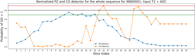
Predictions made on the sequence of Patient WN00001 from the independent testing cohort by PZ-detector (blue) and CG-detector (orange), respectively. Horizontal lines with red, black and green color represent the cutoff of 0.9, 0.8 and 0.7 as the probability of a lesion being malignant.
Figure 8 was one of the successful cases where both CG-detector and PZ-detector were able to pick the suspicious slice and the Grad-CAM (Fig. 9) showed the location of suspicious lesion on that slice which aligned well with the lesion.
Figure 8 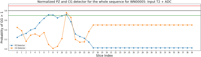
Predictions made on the sequence of Patient WN00005 from the independent testing cohort by PZ-detector (blue) and CG-detector (orange), respectively. Horizontal lines with red, black and green color represent the cutoff of 0.9, 0.8 and 0.7 as the probability of a lesion being malignant.
Figure 9 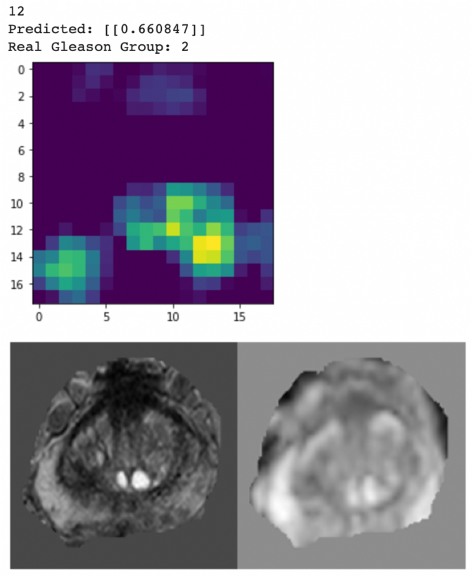
Grad-CAM from the CG-detector indicating PZ-detector and CG-detector were both sensitive to Slice 12 for Patient WN00005, which showed hyper-intense signal in both PZ and CG.
-
(2)
The trained models were verified robust to the domain drift issues caused by ADC map calculated from DWIs with different b values.
-
(3)
By making prediction for each slice and connecting the slices into the sequence, the PZ-detector and CG-detector were able to work together to highlight the suspicious slice out of the sequence.


Conclusions
This work extended our previous research on using deep learning models to read from mpMRI and suggest diagnosis for lesion malignancy. The purpose was one step closer to clinical utilization by means of eliminating the manual efforts of lesion localization, utilizing automatic deep learning framework to search for the optimal augmentation strategy, network architecture and parameters, and finally make prediction for the sequence to find the most suspicious slice and localize the lesion on that slice using the saliency map. The code has been made public and ready to be deployed for anyone who is interested.
Data availability
The datasets used and/or analysed during the current study for testing purpose are available from the corresponding author on reasonable request.
References
Schouten, M. G. et al. Why and where do we miss significant prostate cancer with multi-parametric magnetic resonance imaging followed by magnetic resonance-guided and transrectal ultrasound-guided biopsy in biopsy-naïve men?. Eur. Urol. 71, 896–903 (2017).
Delongchamps, N. B. et al. Multiparametric magnetic resonance imaging for the detection and localization of prostate cancer: Combination of T2-weighted, dynamic contrast-enhanced and diffusion-weighted imaging: INCREASED PROSTATE CANCER DETECTION WITH MULTIPARAMETRIC MRI. BJU Int. 107, 1411–1418 (2011).
Dickinson, L. et al. Magnetic resonance imaging for the detection, localisation, and characterisation of prostate cancer: Recommendations from a European consensus meeting. Eur. Urol. 59, 477–494 (2011).
Sadeghi, Z. et al. MP77-02 a new versus an old notion: Is there any correlation between multi-parametric MRI (MPMRI) PI-RADS (prostate imaging-reporting and data system) score and psa (prostate specific antigen) kinetics?. J. Urol. 199, 1–10 (2018).
Meiers, I., Waters, D. J. & Bostwick, D. G. Preoperative prediction of multifocal prostate cancer and application of focal therapy: Review 2007. Urology 70, S3–S8 (2007).
Tsai, M.-J. & Tao, Y.-H. Machine Learning Based Common Radiologist-Level Pneumonia Detection on Chest X-rays. In 2019 13th International Conference on Signal Processing and Communication Systems (ICSPCS), 1–7 (IEEE, 2019).
Nan, W. et al. Deep neural networks improve radiologists’ performance in breast cancer screening. IEEE Trans. Med. Imaging 39, 1184–1194 (2020).
Armato, G. S. et al. PROSTATEx challenges for computerized classification of prostate lesions from multiparametric magnetic resonance images. J. Med. Imaging 5, 1 (2018).
Liu, S., Zheng, H., Feng, Y. & Li, W. Prostate Cancer Diagnosis Using Deep Learning with 3D Multiparametric MRI. 1013428 (2017).
Tajbakhsh, N. et al. Convolutional neural networks for medical image analysis: Full training or fine tuning?. IEEE Trans. Med. Imaging 35, 1299–1312 (2016).
Litjens, G. et al. A survey on deep learning in medical image analysis. Med. Image Anal. 42, 60–88 (2017).
Deng, J. et al. ImageNet: A large-scale hierarchical image database. In 2009 IEEE Conference on Computer Vision and Pattern Recognition, 248–255 (IEEE, 2009).
Litjens, G., Debats, O., Barentsz, J., Karssemeijer, N. & Huisman, H. Computer-aided detection of prostate cancer in MRI. IEEE Trans. Med. Imaging 33, 1083–1092 (2014).
Zhang, Y., Chan, W. & Jaitly, N. Very deep convolutional networks for end-to-end speech recognition. In 2017 IEEE International Conference on Acoustics, Speech and Signal Processing (ICASSP), 4845–4849 (IEEE, 2017).
Acknowledgements
This work was supported by a Research Scholar Grant, RSG-15-137-01-CCE from the American Cancer Society.
Author information
Authors and Affiliations
Contributions
W.Z. and E.C. conducted the experiment(s), S.Z., E.S., D.C. and J.L. provided contours and medical insights, B.M. and W.W. provided device and funding support. All authors reviewed the manuscript.
Corresponding author
Ethics declarations
Competing interests
The authors declare no competing interests.
Additional information
Publisher's note
Springer Nature remains neutral with regard to jurisdictional claims in published maps and institutional affiliations.
Rights and permissions
Open Access This article is licensed under a Creative Commons Attribution 4.0 International License, which permits use, sharing, adaptation, distribution and reproduction in any medium or format, as long as you give appropriate credit to the original author(s) and the source, provide a link to the Creative Commons licence, and indicate if changes were made. The images or other third party material in this article are included in the article's Creative Commons licence, unless indicated otherwise in a credit line to the material. If material is not included in the article's Creative Commons licence and your intended use is not permitted by statutory regulation or exceeds the permitted use, you will need to obtain permission directly from the copyright holder. To view a copy of this licence, visit http://creativecommons.org/licenses/by/4.0/.
About this article

Cite this article
Zong, W., Carver, E., Zhu, S. et al. Prostate cancer malignancy detection and localization from mpMRI using auto-deep learning as one step closer to clinical utilization. Sci Rep 12, 22430 (2022). https://doi.org/10.1038/s41598-022-27007-y
Received:
Accepted:
Published:
DOI: https://doi.org/10.1038/s41598-022-27007-y
Comments
By submitting a comment you agree to abide by our Terms and Community Guidelines. If you find something abusive or that does not comply with our terms or guidelines please flag it as inappropriate.
