
Abstract
Early detection and appropriate medical treatment are of great use for ear disease. However, a new diagnostic strategy is necessary for the absence of experts and relatively low diagnostic accuracy, in which deep learning plays an important role. This paper puts forward a mechanic learning model which uses abundant otoscope image data gained in clinical cases to achieve an automatic diagnosis of ear diseases in real time. A total of 20,542 endoscopic images were employed to train nine common deep convolution neural networks. According to the characteristics of the eardrum and external auditory canal, eight kinds of ear diseases were classified, involving the majority of ear diseases, such as normal, Cholestestoma of the middle ear, Chronic suppurative otitis media, External auditory cana bleeding, Impacted cerumen, Otomycosis external, Secretory otitis media, Tympanic membrane calcification. After we evaluate these optimization schemes, two best performance models are selected to combine the ensemble classifiers with real-time automatic classification. Based on accuracy and training time, we choose a transferring learning model based on DensNet-BC169 and DensNet-BC1615, getting a result that each model has obvious improvement by using these two ensemble classifiers, and has an average accuracy of 95.59%. Considering the dependence of classifier performance on data size in transfer learning, we evaluate the high accuracy of the current model that can be attributed to large databases. Current studies are unparalleled regarding disease diversity and diagnostic precision. The real-time classifier trains the data under different acquisition conditions, which is suitable for real cases. According to this study, in the clinical case, the deep learning model is of great use in the early detection and remedy of ear diseases.
Introduction
As is known to us all, the sense of hearing is considered as one of the most important five senses, since the sense of hearing is human lives mainly rely on1. However, as a common disease, if not be received early and treated validly, ear disease may leave some negative effects, for example, hearing impairment. In the estimation of ear diseases in the clinic, conventional otoscopy or otoendoscopy is an important component of physical examination at the first step. However, otoscopy or otoendoscopy used in diagnosis can be easily misdiagnosed for non-otolaryngologists2. Research of Pichichero, Poole3, for example, found that the average accuracy of otitis media diagnosed by 514 pediatricians was only 50%. Such low diagnostic accuracy hinted that, without the assistance of supplementary resources, testing the diagnosis of ear disease will be difficult, even for experts. Based on such a situation, there is a great need to find a new diagnostic strategy to improve diagnostic accuracy.
In these years, deep learning has acted as a promising method for image recognition or classification, is the foundation of automatic image perceiving, processing and deciding, and has been a heated topic in the area of computer vision for a long time4,5. Deep learning has been applied in several medical imaging areas, such as the development and validation of a deep learning algorithm for detection of diabetic retinopathy in retinal fundus photographs6, large-scale deep learning for computer-aided detection of mammographic lesions7. What’s more, deep learning has been widely applied in ear and hearing disease classification8,9,10. In these deep learning applications, deep convolutional neural networks (CNNs)4 is playing a very important role in image recognition or classification. Very little prior professional knowledge is needed to input during the training procedure of deep CNNs models. Emerged as a feature extractor, some pre-trained deep CNNs can rival or excel in the execution of domain-specific, handcrafted features11,12,13,14. Comparing to conventional spectral classifiers, deep CNNs is more accurate in image recognition problems due to the millions of weights with multiple layers but have a high computational cost when training the model10,15.
To the best of our knowledge, the purpose of this research is to set up an automatic discriminating system for ear diseases by a deep learning model. The performance of twelve public models was evaluated by accuracy and training-validation time. Based on the assessment results, two best models among 12 models were chosen to build an ensemble classifier which then can design and accomplish a real-time automatic identification of ear diseases system.
Materials and methods
Patient selection and data preprocessing
In this study, our dataset was obtained from 41,056 patients who were diagnosed in the department of otolaryngology in the people's hospital of Shenzhen Baoan District, from July 2016 to August 2019. Usually, patients got their eardrums and external auditory canal (EAC) photos via a conchoscope upon visit. These images were got by using standard endoscopes (Matrix E2, XION GmbH, Berlin, Germany) tethered to Olympus CV-170 digital endovision camera systems (Olympus Corporation, Tokyo, Japan). The resolution rate of these images is 586 × 583 pixels. In order to unify graph data and keep the original shape, we uniformly cropped and scaled these images with a size of 448 × 448 pixels with a ratio of 1:1. We chose 20,542 images, about 53.55% of the total candidate images. Male 11,797. female 8,745. occupied 57.43% and 42.57% of the total number of the selected images, respectively, as shown in Table 1. According to the age, aged (0,10] years have the maximum (22.187%) , aged (30,40] years (21.169%) and (20,30] years (20.861%) in order. Simultaneously, those images were randomly split into three sets, which of 80% for training, 20% for validation, respectively. The training set and validation set have no repetition and are consistent with each model that we trained.
This study confirmed that all methods were implemented in accordance with the relevant guidelines and regulations of the ethics committee of Shenzhen Baoan District People's hospital. It is confirmed that all the experimental protocols have been approved by the ethics committee of Shenzhen Baoan District People's hospital. The informed consent of all subjects was confirmed, and the informed consent of parents and/or legal guardians was obtained for those under 18 years old.
Labeling of images
Image samples of eardrums and EAC were divided into eight categories based on the Colour Atlas of Endo-Otoscopy16, as shown in Fig. 1. All the image classification was implemented by six ear specialists with more than six years of experience. The number of examples representing each ear disease category is shown in Table 2.

Otendoscopy image and eight diagnostic classes of ear diseases. (a) Cholestestoma of middle ear (n = 818). (b) Chronic suppurative otitis media (n = 3169). (c) External auditory cana bleeding (n = 694). (d) Impacted cerumen (n = 5453). (e) Normal eardrum (n = 4217). (f) Otomycosis external (n = 2256). (g) Secretory otitis media (n = 2448). (h) Tympanic membrane calcification (n = 1037).
-
(1)
Normal eardrum and EAC (included completely normal eardrum, normal with healed perforation or some tympanosclerosis, NE, Fig. 2).
Figure 2 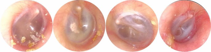
Example of image diversity labelled “Normal”.
-
(2)
Chronic suppurative otitis media (CSOM) There is perforation of tension of tympanic membrane, and they are not a uniform size. Most of them are single shots. The residual tympanic membrane may have calcification, ulceration and granulation tissue growth around the perforation margin.
-
(3)
Cholestestoma of middle ear (CME) Loose inner pocket can be seen, and white exfoliated epithelium can be seen inside the pocket.
-
(4)
External auditory cana bleeding (EACB) Bright red blood can be clearly seen in the external auditory canal.
-
(5)
Impacted cerumen (IC) The external auditory canal can be blocked by brown-black or yellowish-brown lumps. The cerumen masses have different textures, some are loose like mud; some are hard as stone.
-
(6)
Otomycosis external (OE) The external auditory canal and tympanic membrane are covered with yellow black or white powdery or villous fungal masses. The short process of the malleus is apparently exoid.
-
(7)
Secretory otitis media (SOM) The tympanic membrane is invaginated and the handle of the malleus moves backward and upward. When the tympanic cavity has effusion, the tympanic membrane loses its normal luster, showing light yellow, orange oil or amber color, but If the liquid does not fill in the tympanic cavity, the liquid level can be seen through the tympanic membrane.
-
(8)
Tympanic membrane calcification (TMC) The calcification of the tympanic membrane is deposited like white plaque, which is located in the fibrous layer of the tympanic membrane, but the reason is unclear. It may be related to chronic inflammation, such as chronic otitis media and so on, which can be found in the entire intact and perforated tympanic membrane.

Training transfer learning network models
In order to extract features from eardrums and EAC white light images for the automated detection of ear diseases, we used a model method which is typically used to solve image classification in computer vision17,18. In many models of deep learning models, ResNet19 (ResNet50, ResNet101), DensNet-BC20,21 (DensNet-BC121, DensNet-BC161, DensNet-BC169), Inception-V322, V423, Inception-ResNet-V223 and MoblieNet-V224, V325 were implemented and compared performance data from release to release, such as Inputting the image samples, training network, optimizing the network model. Traditionally, the feature maps of the last convolutional layer are vectorized and fed into fully connected layers followed by a softmax logistic regression layer. However, fully connected layers are prone to overfitting. In this process, therefore, we used global average pooling in place of the fully connected layers in each model, generating eight output nodes with a softmax activation function. This have some advantage26: (I) enforcing correspondences between feature maps and categories, thus the features can easily be interpreted as categories confidence maps. (II) No parameter to optimize in the global average pooling. (III) Global average pooling sums out the spatial information thus it is more robust to spatial translations of the input. The training makes full use of a stochastic gradient descent method27 with a batch size of 100, an epoch of 15, an initial learning rate of 0.01, momentum of 0.9 and weight decay of 10–4 to optimize parameters. L2-regularization, dropout and data augmentation were applied to prevent overfitting. The images were flipped horizontally and vertically and then rotated 90 and 180 degrees. Nerves run in various directions, and a change of the nerve direction will not cause any problems.
This study was performed using the deep learning framework PyTorch28 through four graphics processing units (Tesla K80, NVIDIA) in Dell T640 station (inc., USA). For data augment in the process of model training, we performed random X and Y flip horizontal and vertical of input images.
Firstly, we classified the features of image samples of eardrums and EAC from the training sets by feeding to the deep neural network in the frame of PyTorch, and then we observed the performance of the training model on the validation dataset, simultaneously. And when the loss and the accuracy were stable, the training was stopped.
Model structure adjustment
To reduce the size of image features slowly in the convolution operation process of training, we added one dense block ([1 × 1 conv, 3 × 3 conv] × 6) which is the same as the first dense block of DenseNet-BC in the DenseNet-BC20,21 framework (the growth rate is k = 32) and compression is 0.5). Take DensNetBC161 for example, added one dense block ([1 × 1 conv, 3 × 3 conv] × 6) as the first dense block in DensNet-BC161, and the output size is 112 × 112 (tagged as DensNet-BC1615), as shown in Fig. 3. Others, such as, DensNet-BC121 → DensNet-BC1215, DensNet-BC169 → DensNet-BC1915. Therefore, a total of 12 models were implemented and compared performance data from release to release adding the model described above.

A schematic of model structure adjustment for DensNet-BC1615.
Selection of two appropriate models
Through the evaluation of the accuracy and calculation time performance among the 12 models, the appropriate models were selected. 80% and 20% of the images were set up the training set and validation set, respectively, from a total of 20,542 otoendoscopic images. The model optimization step was training-validation which was executed twice with training and validation set respectively.
Ensemble classifier
An ensemble classifier was constructed by combining classifiers' outputs of the two appropriate models. Each classifier model assigns the probability of an input image to eight tags (NE, CME, CSOM, EACB, IC, OE, SOM, TMC) and the maximal probability among all tags is considered as a predictable label. The ensemble classifier combines 8-term score vectors from the predicted results of the two models together and the class with a maximal score will be treated as the final forecast image's label.
Sensitivity–specificity curve
Sensitivity and specificity are frequent clinimetric parameters that together define the ability of a measure to detect the presence or absence of a specific condition (i.e., likelihood ratio). On the whole testing set, a population-level sensitivity and specificity were calculated based on the following formula.
where FP, PN, TP and PN represent the numbers of false positives, false negatives true positives and true negatives, respectively. A sensitivity–specificity curve can be created by changing the threshold value t (probability p ≥ t, where t is a threshold value).
Confusion matrix
We used the confusion matrix to evaluate the quality of the output of the classifier. The values in the diagonal line represent the number of correctly predicted samples, while the values not in the diagonal elements represent the number of misclassified samples. If the diagonal values are very high, it indicates the classifier has a very good performance.
Overall accuracy
The overall accuracy is the ratio of the number of correctly categorized images to the total number of testing images, as shown below:
Results
Model and performance analysis
The number of parameters, training and validation time (Model optimization time) and accuracy of every transferred model were revealed in Table 3. The number of parameters was calculated by user-defined python programs, as shown below.
def get_model_parameter_num(net):
total_num = sum(p.numel() for p in net.parameters())
trainable_num = sum(p.numel() for p in net.parameters() if p.requires_grad)
return {'Total Time': total_num, 'Train Time': trainable_num}
The hidden layer of the models had no significant improvement. There is not a hidden layer in the fully connected layer of the ten models. Calculating results show that the best accuracy was the DenseNet-BC1615 (95.099%), followed by Inception-ResNet-V2 (94.617%), DenseNet-BC161(94.564%) and DenseNet-BC169 (94.541%), as shown in Table 3. For model optimization time, DenseNet-BC1615, Inception-ResNet-V2, DenseNet-BC161 and DenseNet-BC169 were 80,895, 111,849 and 78,453 and 56,477 s, respectively. In order to test the stability of the model, the 12 models which we have been trained were evaluated by 10 percent of the sample which collected randomly from the training set. Repeated the previous step ten times and recorded its accuracy, and then and then performed repeated measures one-way ANOVA, as shown in Fig. 4a. One-way ANOVA indicated that the DensNet-BC1615 and DensNet-BC169 increased more significantly than other models except for the Inception-ResNet-V2 (the reason it was not chosen was that it took too long to train). Then we analyzed the significance of the two models we selected and the best two of the remaining models. It further showed that the two models increased diagnostic accuracy significantly (p-value = 2.74e−09), as shown in Fig. 4b.

The accuracy comparison between different models on 10 sampling datasets.
Together with the accuracy and the model optimization time, DenseNet-BC1615 and DenseNet-BC169 were selected to be the best-transferred network models to form an ensemble classifier. To better display the training process, we add learning curves to visualize the training performance of these 2 selected deep learning models (Fig. 5).

The learning curves of 2 selected models, DenseNet 1615 (a) and DenseNet 169 (b).
From the two models, the classification mechanism of the ensemble classifier is estimated according to the following formula.
where S1 and S2 are the lexicographic vector of an input image predictor score of the two models, respectively. S1*S2 represents the dot product of the S1 and S2 vectors. S is a predicted label score of the ensemble classifier. For this design, we also give an example of the ensemble classifier running results which were shown in Fig. 6.

A sketch of structure and an operating diagram for the ensemble method classifies given otoendoscopic image.
In this research, we calculated the confusion matrices for DensNet-BC1615, DensNet-BC169 and the ensemble classifier that were shown in Fig. 7. These results are obtained by identifying the testing data with these 3 models. The testing data covers 10% of total images and is not used during the whole training process. The average classification accuracy was obtained on DensNet-BC1615, DensNet-BC169 and the ensemble classifier reached 94.94%, 95.08%, and 95.59%, respectively. The combined forecasting method possessed the two single method's advantages, and the result showed that forecast value was more accurate.

Confusion matrices for DensNet-BC169, DensNet-BC1615, and ensemble classifier at the test sample sets having a maximal accuracy.
We assessed the ensemble classifier according to the performance of generating binary predictions on Urgent versus Non-urgent subjects. Blood transfusion is the means of life-saving treatment of many diseases. Such a binary classification task has been very important for clinical significance since emergency cases should be treated immediately. Any delay, attributed to misclassification, for example, will increase the risk of death. The performance of the Urgent versus Non-urgent based on the sensitivity–specificity curve can be clearly found in Fig. 8. The AUCs of the DensNet-BC1615, DensNet-BC169 and the ensemble classifier were 0.9968, 0.9965, and 0.9974, respectively. The reason for the increase in the overall accuracy of the ensemble classifier is that the ensemble classifier actually can classify more samples correctly based on the result of two separate models. For example, one sample gets wrong identification by one model but obtains the correct label in another model, in this case, the ensemble classifier can eventually return the correct classification result to this sample. As a result, more samples can get correct classification by using an ensemble classifier.

The sensitivity–specificity curve of the ensemble classifier at the test sample sets for Urgent versus Non-urgent binary classification.
The real-time automatic identification system
A real-time automatic identification system was designed by combining an endoscopy system and ensemble classifier, as shown in Fig. 7, and its web page also can be seen in. The image was obtained from the endoscopy system by adjusting the focus. The image got into the real-time recognition system after being processed by the capture system, and then the prediction results were obtained by the ensemble classifier, which was displayed on the web page of the system. Provided that an image is in the process of real-time classification if the maximum probability of the eight classes (NE, CME, CSOM, EACB, IC, OE, SOM, TMC) estimated by one of the three models (DenseNet-BC169, DenseNet-BC1615 and ensemble classifier) is less than or equal to 0.3, or more than three categories of the prediction probabilities are greater than 0.3 in any model of the three, the system would point out that the image is likely to be excluded in those eight categories and give tips on the web page of the system (others, as shown in the inset of Fig. 9), which will arouse doctors' attention and give artificial intervention to avoid misjudgment.

A schematic diagram of the real-time automatic identification system for ear diseases and the system web page of the system. The red border is drawn manually by the doctor.
In addition, to test the working stability of the real-time automatic identification system, we do a general analysis of the confusion matrices and the sensitivity–specificity curve using the clinical endoscopic images of the department of otolaryngology in the people's hospital of Shenzhen Baoan district in the past six months, as shown in Fig. 10. The average classification accuracy and the AUCs were 95.127% and 0.9949, respectively. The actual test shows that the system achieves the desired objective and is stable and reliable. The response forecast time of the system is about 0.7 s for one endoscopic image.

The Confusion matrices (a) and sensitivity–specificity (b) curve of the real-time automatic identification system based on the ensemble classifier at endoscopic images about the past six months.
Discussion
Diagnosis of ear disease mainly depends on otoscopy and physician's experience29, especially external auditory canal. For the accuracy of the ear disease diagnosis, otolaryngologists executed demonstrably better than pediatricians and general practitioners, because diagnosis by otoendoscopy needed expertise in otology doctors30. In this condition, the deep network model could provide physicians with suggesting potential diagnosis according to otoendoscopic image8,9,31.
In the current model, a dataset of 20,542 labeled otoendoscopic images from more than 40,000 patients was used. Otoendoscopic images of the eardrum and external auditory canal were classified into six categories. The classification accuracy of the current model has reached 95.59%. Previous studies make use of 10,544, 389 and 391 images to analyze ear diseases, with the accuracy of 93.73%, 86.84% and 80.6%31,32,33, respectively. Unluckily, this is only for scientific research and has not been translated into applications. In our work, we also build a real-time interactive detection system that provides doctors with real-time diagnostic results for complementary medical benefits. The classification accuracy of our model reached 95.59%.
There are a few notable limitations to this study. These include the collection of the video frame by a simple operator who is also an acknowledged expert in otology and the use of video frame recordings instead of real-time assessments of ear disease. Nevertheless, we hope that the competence to operate and stabilize the instrument to let stable imaging of the eardrum and external auditory canal in focus will be obtainable by an otoscope inspector with a generally-used skill. Even though this is not the real-time detecting of the eardrum and external auditory canal in clinical treatment because this model has not yet been utilized in an actual patient deployment scenario, as is mentioned above, the testing dataset is untouched, raw and our model executes in almost real-time.
Looking ahead, an approach similar to deep learning also has great potential in improving endoscopic otologic diagnosis. In addition, alternative endoscopic images, confocal laser and endocytoscopy, for example, are most likely to be utilized to train this platform to supply an explanation of clinically acquired images.
In summary, this study shows that a real-time deep learning system of ear disease diagnosis according to otoscopy can realize high accuracy in sorting the disease of the eardrum and external auditory canal when used on unaltered otoscopy, video sequences. Given its high accuracy, we plan to conduct clinical trials to assess the potential of this imaging analytics artificial intelligence model in day-to-day practice. For possible future works, we plan to adapt our method to other kinds of medical images like rhinoscopes or laryngoscopes. Besides, we also plan to develop our method to desktop software, which could be a very useful aided tool for the diagnosis of ear disease.
References
Naser, S. S. A. & Hasanein, H. A. A. Ear diseases diagnosis expert system using SL5 object. World Wide J. Multidiscipl. Res. Dev. 2, 41–47 (2016).
Blomgren, K. & Pitkäranta, A. Is it possible to diagnose acute otitis media accurately inprimary health care?. Fam. Pract. 20, 524–527 (2003).
Pichichero, M. E. & Poole, M. D. Assessing diagnostic accuracy and tympanocentesis skills in the management of otitis media. Arch. Pediatr. Adolesc. Med. 155, 1137–1142 (2001).
LeCun, Y., Bengio, Y. & Hinton, G. Deep learning. Nature 521, 436–444 (2015).
He, K., Zhang, X., Ren, S., et al. Delving deep into rectifiers: surpassing human-level performance on ImageNet classification. in Proceedings of the IEEE International Conference on Computer Vision. https://www.cv-foundation.org/openaccess/ (2015).
Kooi, T. et al. Large scale deep learning for computer-aided detection of mammographic lesions. Med. Image Anal. 35, 303–312 (2017).
Gulshan, V. et al. Development and validation of a deep learning algorithm for detection of diabetic retinopathy in retinal fundus photographs. JAMA Intern. Med. 316, 2402–2410 (2016).
Vaidyanathan, A. et al. Deep learning for the fully automated segmentation of the inner ear on MRI. Sci. Rep. 11, 2885 (2021).
Senaras, C., Moberly, A. C., Teknos, T., Essig, G., Elmaraghy, C., Taj-Schaal, N., Yua, L., Gurcan, M. N. Detection of eardrum abnormalities using ensemble deep learning approaches. in Proc. SPIE 10575, Medical Imaging: Computer-Aided Diagnosis, 105751A (2018).
Anwar, S. M. et al. Medical image analysis using convolutional neural networks: A review. J. Med. Syst. 42, 226 (2018).
Gong, Y. et al. Multi-scale orderless pooling of deep convolutional activation features. In Computer Vision-ECCV (eds Fleet, D. et al.) (Springer, 2014).
Sharif Razavian, A., Azizpour, H., Sullivan, J., et al. CNN features off-theshelf: an astounding baseline for recognition. in Proceedings of the IEEE Conference on Computer Vision and Pattern Recognition Workshops. https://www.cv-foundation.org/openaccess/ (2014).
Cimpoi, M., Maji, S., Vedaldi, A. Deep filter banks for texture recognition and segmentation. in Proceedings of the IEEE Conference on Computer Vision and Pattern Recognition. https://openaccess.thecvf.com/ (2015).
Sermanet, P., Eigen, D., Zhang, X. et al. Overfeat: Integrated recognition, localization and detection using convolutional networks. https://arxiv.org/abs/1312.6229 (2017).
Prakash, N., Manconi, A. & Loew, S. Mapping landslides on EO data: Performance of deep learning models vs traditional machine learning. Models. Remote Sens. 12, 346 (2020).
Sanna, M., Russo, A., Caruso, A., Taibah, A., Piras, G. Color atlas of endo-otoscopy. Examination-Diagnosis-Treatment, 8–11, 14–54, 66–74, 81–92, 94–112, 118–138, 160–166, 195–197 (2017).
Ren, S. et al. Faster R-CNN: Towards real-time object detection with region proposal networks. Neural Inf. Process. Syst. 28, 91–99 (2015).
Li, J. et al. Computer-assisted detection of colonic polyps using improved faster R-CNN. Chin. J. Electron. 28, 718–724 (2019).
He, K., Zhang, X., Ren, S., Sun, J. Deep residual learning for image recognition. Proceedings of the IEEE conference on computer vision and pattern recognition, https://arxiv.org/ (2016).
Huang, G., Liu, Z., Der Maaten, L. V., Weinberger, K. Q. Densely Connected Convolutional Networks. in Proceedings of the IEEE computer vision and pattern recognition. https://arxiv.org/abs/1608.06993 (2017).
Pleiss, G., Chen, D., Huang, G. et al. Memory-efficient implementation of densenets. https://arxiv.org/abs/1707.06990 (2017).
Szegedy, C., Vanhoucke, V., Ioffe, S., Shlens, J., Wojna, Z. Rethinking the inception architecture for computer vision. in Proceedings of the IEEE conference on computer vision and pattern recognition. https://arxiv.org/abs/1512.00567 (2016).
Szegedy, C., Ioffe, S., Vanhoucke, V., Alemi, A.A. Inception-v4, Inception-ResNet and the Impact of Residual Connections on Learning. Thirty-first AAAI conference on artificial intelligence. https://arxiv.org/abs/1602.07261 (2017).
Sandler, M., Howard, A., Zhu, M. et al. Mobilenetv2: Inverted residuals and linear bottlenecks. Proceedings of the IEEE conference on computer vision and pattern recognition. https://arxiv.org/abs/1801.04381 (2018).
Howard, A., Sandler, M., Chu, G., et al. Searching for MobileNetV3. International conference on computer vision. https://ieeexplore.ieee.org/document/9008835 (2019).
Lin, M., Chen, Q., Yan, S. Network in network. https://arxiv.org/abs/1312.4400 (2013).
Bottou, L. Large-scale machine learning with stochastic gradient descent. in Proceedings of COMPSTAT'2010 (Lechevallier Y., Saporta G., eds) (Physica-Verlag HD, 2010). https://doi.org/10.1007/978-3-7908-2604-3_16.
Ketkar, N. Introduction to PyTorch. in Deep Learning with Python. (Apress, 2017). https://doi.org/10.1007/978-1-4842-2766-4_12.
Marom, T., Kraus, O., Habashi, N. & Tamir, S. O. Emerging technologies for the diagnosis of otitis media. Otolaryngol. Head. Neck Surg. 160, 447–456 (2019).
Pichichero, M. E. & Poole, M. D. Comparison of performance by otolaryngologists, pediatricians, and general practioners on an otoendoscopic diagnostic video examination. Int. J. Pediatr. Otorhinolaryngol. 69, 361–366 (2005).
Cha, D., Pae, C., Seong, S., Young Choi, J. & Park, H. Automated diagnosis of ear disease using ensemble deep learning with a big otoendoscopy image database. EBioMedicine 45, 606–614 (2019).
Myburgh, H. C., van Zijl, W. H., Swanepoel, D., Hellstrom, S. & Laurent, C. Otitis media diagnosis for developing countries using tympanic membrane image-analysis. EBioMedicine 5, 156–160 (2016).
Myburgh, H. C., Jose, S., Swanepoel, D. W. & Laurent, C. Towards low cost automated smartphone- and cloud-based otitis media diagnosis. Biomed. Signal. Process. Control 39, 34–52 (2018).
Funding
This work is supported by the foundation for young creative talents of department education of Guangdong (Natural Science), China, Grant No. 2019KQNCX067.
Author information
Authors and Affiliations
Contributions
X.Z., H.G. Li, F.W. and Z.L. designed the study, collected the data, analyzed the data and wrote the manuscript. J.S., K.W., T.L. and X.L. collected the data. W.L. and Z.J. designed a deep transfer learning system and performed training with Z.L. H.Y. Li, G.L and Z.J. designed and developed a real-time automatic identification system. All authors read and approved the final version of the manuscript.
Corresponding authors
Ethics declarations
Competing interests
The authors declare no competing interests.
Additional information
Publisher's note
Springer Nature remains neutral with regard to jurisdictional claims in published maps and institutional affiliations.
Rights and permissions
Open Access This article is licensed under a Creative Commons Attribution 4.0 International License, which permits use, sharing, adaptation, distribution and reproduction in any medium or format, as long as you give appropriate credit to the original author(s) and the source, provide a link to the Creative Commons licence, and indicate if changes were made. The images or other third party material in this article are included in the article's Creative Commons licence, unless indicated otherwise in a credit line to the material. If material is not included in the article's Creative Commons licence and your intended use is not permitted by statutory regulation or exceeds the permitted use, you will need to obtain permission directly from the copyright holder. To view a copy of this licence, visit http://creativecommons.org/licenses/by/4.0/.
About this article

Cite this article
Zeng, X., Jiang, Z., Luo, W. et al. Efficient and accurate identification of ear diseases using an ensemble deep learning model. Sci Rep 11, 10839 (2021). https://doi.org/10.1038/s41598-021-90345-w
Received:
Accepted:
Published:
DOI: https://doi.org/10.1038/s41598-021-90345-w
This article is cited by
-
An ensemble approach for classification of tympanic membrane conditions using soft voting classifier
Multimedia Tools and Applications (2024)
-
Insight into Automatic Image Diagnosis of Ear Conditions Based on Optimized Deep Learning Approach
Annals of Biomedical Engineering (2024)
-
Auto-metric distribution propagation graph neural network with a meta-learning strategy for diagnosis of otosclerosis
Applied Intelligence (2024)
Comments
By submitting a comment you agree to abide by our Terms and Community Guidelines. If you find something abusive or that does not comply with our terms or guidelines please flag it as inappropriate.
