
Abstract
In order to study the influence of distance weight on ore-grade estimation, the inverse distance weighted (IDW) is used to estimate the Ni grade and MgO grade of serpentinite ore based on a three-dimensional ore body model and related block models. Manhattan distance, Euclidean distance, Chebyshev distance, and multiple forms of the Minkowski distance are used to calculate distance weight of IDW. Results show that using the Minkowski distance for the distance weight calculation is feasible. The law of the estimated results along with the distance weight is given. The study expands the distance weight calculation method in the IDW method, and a new method for improving estimation accuracy is given. Researchers can choose different weight calculation methods according to their needs. In this study, the estimated effect is best when the power of the Minkowski distance is 3 for a 10 m × 10 m × 10 m block model. For a 20 m × 20 m × 20 m block model, the estimated effect is best when the power of the Minkowski distance is 9.
Introduction
The inverse distance weighted (IDW) method as an interpolation method1. Widely used in, image interpolation2, spatial data interpolation3,4, and algorithm optimization5,6. The IDW method is considered to be a highly adaptable resource estimation method7. Studies focusing on the IDW method as a resource estimation tool focus on two aspects: estimating natural recourses and improving the IDW method. The IDW method has been used to estimate grade8,9, such as Cu and Mo10. On the other hand, a significant amount of research has been done on improving the IDW method. The weight coefficient distribution was refined, and the estimation accuracy was improved by modifying the weight of the angle weight coefficient11. The IDW method was further improved to consider directionality and extrapolate data12. Researchers proposed the Indicated-IDW, which reported and improved estimation accuracy13. The improvements reflect the anisotropic characteristics of ore grade; however, its application scope is limited.
The IDW method is a biased estimation method14; however, there is little research on the systematic deviation of IDW estimation. The authors estimate Ni and MgO grades of serpentinite ore with the starting of the above question, introduce Minkowski distance as the distance weight of IDW and examine the effect of distance weight and grade distribution on estimation deviation. The distance weight calculation method is extended, and system estimation grade deviations for different distance weights are given.
Data sources and research methods
Overview of the study area
The study area is located on the southern margin of the Sino-Mongolian trough. The NE-trending and NW-trending structures in the area constitute the overall tectonic framework of the mining area. The rock type is basic-ultrabasic, with intrusive rocks being the most common rock type. Serpentinite ore bodies occur in the Carboniferous Benbantu Formation (C2bb) tuffaceous slate, specifically the No. 1 and No. 2 ore bodies. In this study, the No. 1 ore body was used for example. The No. 1 serpentinite ore body has the length of 1166 m, a maximum control depth of 590 m, a strike of 108°, the inclination angle is 198°, an inclination angle of 9–26°, and average inclination angle of 17°.The true thickness of ore body is between 26.53 and 145.19 m, with an average thickness of 91.47 m. Thickness changing coefficient of the ore body is 45%.
Data collection and processing
-
(1)
Ore body model and block model
Serpentine ore physical parameters are used to build a three-dimensional model of the ore body (Fig. 1), and two types of corresponding block models. Model 1 has a block size of 10 m × 10 m × 10 m and contains 50,638 blocks. Model 2 has a block size of 20 m × 20 m × 20 m and contains 7532 blocks (Fig. 2).
Figure 1 
3D model of ore body.
Figure 2 
Block model.
-
(2)
Sample grade statistics
188 serpentinite ore samples were subjected to ore-grade estimation. Samples were collected in past exploration projects. Figures 3 and 4 show the Ni and MgO grade histograms respectively.
Figure 3 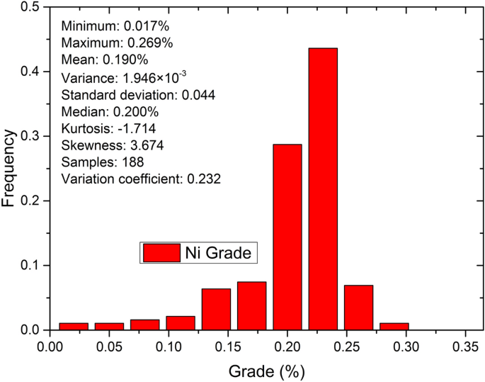
Grade distribution of Ni samples.
Figure 4 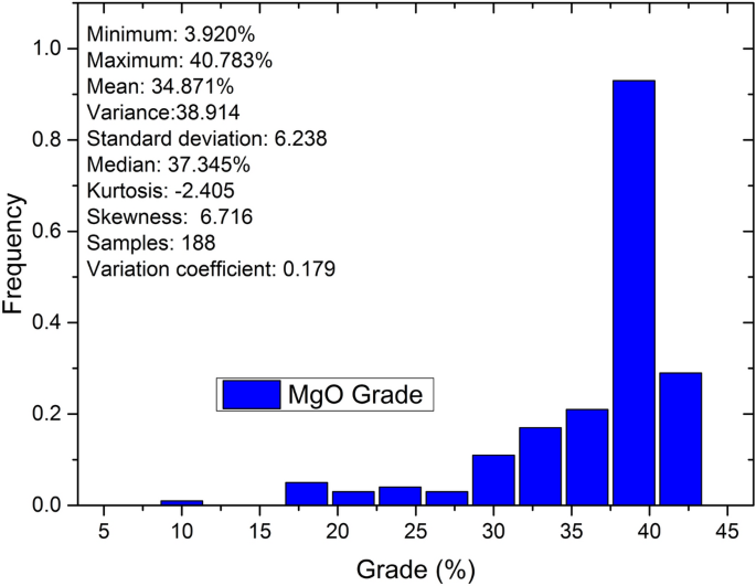
Grade distribution of MgO samples.


Research methodology
The IDW method is a spatial interpolation method15, which uses spatial distance for the correlation calculation that is the distance weight calculation. For an unknown point P with position (x0, y0, z0), there are known points around it. Assuming that each known point has spatial coordinates of (xi, yi, zi) (i = 1, 2, …, n), and the attribute value is Pi. The distance between each known point and unknown point is di(x, y, z). IDW is used to estimate the property value of each unknown point. Equation (1) represents this estimation16. In Eq. (1), m is the power in the inverse distance power law.
In the study, the special form of Minkowski distance17 is used in the distance weight calculation method of IDW. Minkowski distance is expressed as:
where p is the power of the Minkowski distance, and p can be 0 to + ∞. When p = 1, it is the Manhattan distance18,19. It is expressed as:
When p = 2, it is Euclidean distance. It is expressed as:
When p → + ∞, it is Chebyshev distance. It is expressed as:
The study also involves a number of sample points (n in Eq. (1), the value is 3), the distance power (m in Eq. (1), value is 2), and search radius (value is 300 m). Estimation deviation is a method of comparing estimated grade to sample grade. The deviation is calculated as: deviation = (estimation grade − sample grade)/sample grade × 100%.
Results and analysis
Estimated grades of Ni and MgO are given in Tables 1 and 2.
The estimated grade and sample grade are compared. Figures 5, 6, 7, and 8 represent the estimated deviation in minimum, maximum, average, and standard deviations. The horizontal axis corresponds to Manhattan distance (p = 1), Euclidean distance (p = 2), Minkowski distance (p = 3, 5, 7, 9, 11, 13, 15), and Chebyshev distance (p → ∞) (Figs. 5, 6, 7, 8).

Deviation of minimum ore grade.

Deviation of maximum ore grade.

Deviation of average ore grade.

Deviation of ore grade standard deviation.
The minimum deviation of Ni is less than the minimum deviation of MgO (Fig. 5). Grade distribution and model type have an effect on the estimated IDW results. The sample proportion is only 12.23% with the sample Ni grade between 0.017 and 0.140%. The sample proportion is only 7.45% with MgO grade between 3.92 and 24%.Three samples are used to estimate an unknown point in the estimate. The probability of 3 samples simultaneously being low grade is small, resulting in a larger minimum valuation deviation. Therefore, the deviation of the minimum value is larger. Since the proportion of Ni is larger than that of MgO in the low-grade section, the deviation of MgO grade minimum is greater than that of the Ni grade. The estimated grade minimum deviation from Model 1 is larger than that of Model 2. This may be due to fewer number of samples in the area where the sampled value is lower. The low-grade sample control area is large.
The influence of distance weight on the maximum grade deviation is small (Fig. 6).The maximum deviation of the Ni and MgO estimated grades is negative, indicating that the maximum estimated Ni and MgO grades is less than the maximum sample grade. The Ni maximum grade deviation is greater than that of MgO maximum grade in model 1. Ni grade maximum deviation varies greatly in Manhattan distance, Euclidean distance, and Minkowski distance (p = 3–5) within model 2. Minkowski distance maximum deviation (p = 5–∞) is relatively stable at approximately 2.89%. MgO grade maximum deviation jumps at p = 13–15 and ranges in absolute value from large to small. The maximum deviation after the change is close to Ni in model 1. Therefore, the sample grade distribution and model type has an influence on the estimated results. The lower grade maximum deviations are due to the higher number of high-grade samples, which is the opposite a deviation in minimum grade.
The Ni and MgO grade average deviations clearly form two groups according to model 1 and model 2 (Fig. 7). The average estimated grade is less than the sample grade, when the Minkowski distance power is less than 20 (p < 20) in model 1. When Chebyshev distance is used, the average estimated grade is more than the sample grade in model 1. The average estimated grade is less than the sample grade in model 2. The average MgO grade deviation is slightly less than the average Ni grade deviation in models 1 and 2, showing that the estimated deviations for the IDW method are related to the calculation method, distance weight, and sample distribution. The average deviation of model 1 is less than model 2, indicating that block size has an influence on the estimate results and a greater block size bring about a greater average deviation. When Minkowski distance is used to calculate distance weights and p < 20, Ni and MgO grades are at risk of being under estimated within model 1. When Chebyshev distance is used, Ni and MgO are at risk of being over estimated. Ni and MgO grades are at risk of being under estimated within model 2.
Deviations in the standard deviation of Ni and MgO grades are presented in two groups according to model 1 and model 2 (Fig. 8). The trend of the deviation in standard deviation is exactly the opposite of the average deviation trend. When the Minkowski distance power is less than 11 (p < 11), deviations in standard deviation are stable in model 1 and are relatively unstable in model 2. When the Minkowski distance power is greater than 11, deviations in standard deviation rapidly increase in model 1 and change from positive to negative in model 2, which is consistent with the trend of model 2. Therefore, deviations in the standard deviation of Ni grade and MgO grade are different, showing that estimated results of the IDW method are affected by the distance weight calculation method and grade distribution. In addition, the trend of the deviation in standard deviation of Ni and MgO is consistent within a given model, indicating that block size has a significant impact on the estimate results.
A comprehensive analysis of the estimated deviation indicates that the estimated ore grade results are regular in the IDW method which uses the Minkowski distances to calculate weights. The effect of the distance weight calculation method on the IDW method is confirmed by the two models. The effect of block size on the estimated result is also significant. The estimation is best in model 1when p = 3.At this time, the average Ni grade deviation is − 3.77%, and the average MgO grade deviation is − 2.99%. The estimation is best in model 2 when p = 9. At this time, the average Ni grade deviation is − 7.22%, and the average MgO grade deviation is − 8.09%.
Discussion
The IDW method is widely used as a highly adaptive grade estimation method. Previous research seldom examined the distance weight calculation method and estimated system deviation of the IDW method. Estimated grade deviations show that Euclidean distance is not the best option for distance weight calculations; therefore, it is necessary to study the influence of other distance weight calculation methods.
Ni and MgO samples are from the same exploration project, and all samples were collected in the same way; however, when the same distance weight is used, the estimated deviations are not the same. Hence ore grade distribution must have an influence on the estimated results. The variation in the two types of estimated grade deviations is consistent, indicating that the estimated results of IDW are stable for different distance weights. Two model sizes are used to verify the effect of the distance weight calculation method on Ni and MgO grade estimated results. The IDW estimated results of Ni and MgO grade are also divided into two groups according to the two models. The deviations in average and standard deviation of Ni and MgO grade and are consistent for the same block model, which further clarifies the effect of distance weights on IDW estimated results.
This study theoretically expands the calculation method for the distance weight of the IDW method. The Euclidean distance weight is extended to the use of Minkowski distance weight, and a new optional parameter (distance weight) is added. The deviations of the estimated system are given when the Minkowski distance weight is used. This new method can improve ore-grade estimation by choosing the Minkowski distance power value. More study is needed to further verify the effect of the distance weight calculation method on ore-grade estimation, especially the influence of distance weight and grade distribution in the IDW method.
Conclusion
-
(1)
The estimated effect of the Ni and MgO grades is clearly presented in two groups according to block models based on IDW method along with the distance weight. The Ni and MgO grade estimation deviations have high consistency for the same block model, indicating that the distance weight calculation method has a significant impact on IDW. Estimated Ni and MgO grades in serpentinite show that it is feasible to use Minkowski distance for the distance weighting in the IDW method. The study expands the calculation method for distance weight using IDW and gives the variation rule for the estimated Ni and MgO grade deviation with Minkowski distance. The law of the estimated results along with the distance weight is given.
-
(2)
This study expands the calculation method for the distance weight in the IDW method and provides a new way to improve estimation accuracy by choosing the distance weight calculation method. Ore-grade estimation of serpentinite deposits shows that the Minkowski distance provides the best estimation when a power of 3 is used within model 1. At this time, the Ni and MgO grade average deviations are − 3.77% and − 2.99%, respectively. The Minkowski distance provides the best Ni and MgO grade estimation when a power of 9 is used within model 2. At this time, the average deviations are − 7.22% and − 8.09%, respectively.
References
Chen, C., Zhao, N., Yue, T. & Guo, J. A generalization of inverse distance weighting method via kernel regression and its application to surface modeling. Arab. J. Geosci. 8, 6623–6633 (2015).
Jing, M. & Wu, J. Fast image interpolation using directional inverse distance weighting for real-time applications. Opt. Commun. 286, 111–116 (2013).
Chen, F. W. & Liu, C. W. Estimation of the spatial rainfall distribution using inverse distance weighting (IDW) in the middle of Taiwan. Paddy Water Environ. 10, 209–222 (2012).
Emine, T. K. & Selma, Z. K. Comparison of regression-based and combined versions of inverse distance weighted methods for spatial interpolation of daily mean temperature data. Arab. J. Geosci. 9, 690–699 (2016).
He, Y., Zhang, B. & Yao, E. Weighted inverse minimum spanning tree problems under hamming distance. J. Combinat. Optimization 9, 91–100 (2005).
Gholipour, Y., Shahbazi, M. M. & Behnia, A. An improved version of inverse distance weighting metamodel assisted Harmony Search algorithm for truss design optimization. Latin Am. J. Solids Struct. 10, 283–300 (2013).
Shahbeik, S., Afzal, P. & Parviz, M. Comparison between ordinary Kriging (OK) and inverse distance weighted (IDW) based on estimation error. Case study: Dardevey iron ore deposit, NE Iran. Arab. J. Geosci. 7, 3693–3704 (2014).
Song, Y. C., Liu, Z. N., Meng, H. D. & Zhang, P. W. Influence of determination method of volumetric weight of ore on reserves estimation: Taking an iron & copper mine as a case. Metal Mine 40, 106–109 (2015).
Runtang, J., Fan, Y., Yanmei, W. & Yanwei, H. Reserve estimation and establishment of three-dimensional geological model of Bairong-gangjiangcu (Mo) deposit, Tibet. Metal Mine 40, 95–99 (2015).
Bingsheng, W. U. & Li, S. U. Resource estimation of deposit based on Surpac software and geostatistics. Mining Res. Dev. 35, 88–91 (2015).
Tie, W., Zhiqiu, J. & Zhihong, W. Improvement and parameter optimization of distance power inverse ratio method. China Mining Magaz. 3, 47–50 (1994).
Ziling, S. The calculation method of geology reserve of the coal mine beds a improved distance power estimating method in geoloogic model. J. Liaoning Tech. Univ. 16, 339–341 (1997).
Fu-Kun, Z., Han, W. & Ke-Jun, Z. Combinatorial optimization of oil field development plan based on topsis with different distance. Math. Practice Theory 45, 158–164 (2015).
Yang, J. F., Zhou, S. X. & Xue, L. P. Three dimensional geological modeling and reserves estimation of HuiliLalacopper mine based on Dimine. Metal Mine 41, 114–118 (2016).
Zhanglin, L., Xialin, Z., Gang, L. & Chonglong, W. Automatically optimizating the participant samples by inverse distance weighting method. Geol. Sci. Technol. Inf. 33, 209–212 (2014).
Ping, D., Yehua, S., Jia, L. I., Haiyang, L. V. & Siyang, Z. Adaptive IDW interpolation method and its application in the temperature field. Geogr. Res. 196, 31–38 (2014).
Yang, F., Guo, J. H. & Tan, H. Comparison of similarity measurement of SIF feature descriptor based on different distance measures. Remote Sens. Inf. 32, 104–108 (2017).
Zhanglin, L., Ping, W. & Xialin, Z. Improvement and application of inverse distance weighted method. Metal Mine 32, 88–92 (2008).
Chen, J. G. Particl velocity detection technology based on manhattan distance method. Ind. Mine Automat. 41, 52–55 (2015).
Acknowledgements
This work is supported by PhD Research Startup Foundation (No. BSJ2021003) of Anyang Institute of Technology. Thanks to the National Natural Science Foundation of China (No. 71363040), the Science and Technology Development Project of Henan Province in 2021 (No. 212400410251) and the R&D and Promotion Key Program of Anyang in 2020 (No. 2020-256) for their support for this study. Thanks are due to Yu-Cheng Song and Hai-Dong Meng for their initial suggestions and inspiration.
Author information
Authors and Affiliations
Contributions
Z.-N.L. designed and performed the experiment and wrote the paper, X.-Y.Y. processed the data and pictures, L.-F.J. and Y.-S.W. revised the paper. Y.-C.S. and H.-D.M. guided the research.
Corresponding author
Ethics declarations
Competing interests
The authors declare no competing interests.
Additional information
Publisher's note
Springer Nature remains neutral with regard to jurisdictional claims in published maps and institutional affiliations.
Rights and permissions
Open Access This article is licensed under a Creative Commons Attribution 4.0 International License, which permits use, sharing, adaptation, distribution and reproduction in any medium or format, as long as you give appropriate credit to the original author(s) and the source, provide a link to the Creative Commons licence, and indicate if changes were made. The images or other third party material in this article are included in the article's Creative Commons licence, unless indicated otherwise in a credit line to the material. If material is not included in the article's Creative Commons licence and your intended use is not permitted by statutory regulation or exceeds the permitted use, you will need to obtain permission directly from the copyright holder. To view a copy of this licence, visit http://creativecommons.org/licenses/by/4.0/.
About this article

Cite this article
Liu, ZN., Yu, XY., Jia, LF. et al. The influence of distance weight on the inverse distance weighted method for ore-grade estimation. Sci Rep 11, 2689 (2021). https://doi.org/10.1038/s41598-021-82227-y
Received:
Accepted:
Published:
DOI: https://doi.org/10.1038/s41598-021-82227-y
This article is cited by
-
An observation study of the combined river discharge and sea level impact on the duration of saltwater intrusion in Pearl River estuary–Modaomen waterway
Natural Hazards (2024)
-
Soil quality assessment in low human activity disturbance zones: a study on the Qinghai-Tibet Plateau
Environmental Geochemistry and Health (2024)
-
A new method for estimating ore grade based on sample length weighting
Scientific Reports (2023)
-
Research on dimensionality reduction in unconstrained face image based on weighted block tensor sparse graph embedding
Signal, Image and Video Processing (2023)
-
Influence of adaptive inverse distance weighting method under membership function mapping on the interpolation accuracy of geological boreholes
Earth Science Informatics (2023)
Comments
By submitting a comment you agree to abide by our Terms and Community Guidelines. If you find something abusive or that does not comply with our terms or guidelines please flag it as inappropriate.
