
Abstract
Ribosomal RNAs are complex structures that presumably evolved by tRNA accretions. Statistical properties of tRNA secondary structures correlate with genetic code integration orders of their cognate amino acids. Ribosomal RNA secondary structures resemble those of tRNAs with recent cognates. Hence, rRNAs presumably evolved from ancestral tRNAs. Here, analyses compare secondary structure subcomponents of small ribosomal RNA subunits with secondary structures of theoretical minimal RNA rings, presumed proto-tRNAs. Two independent methods determined different accretion orders of rRNA structural subelements: (a) classical comparative homology and phylogenetic reconstruction, and (b) a structural hypothesis assuming an inverted onion ring growth where the three-dimensional ribosome’s core is most ancient and peripheral elements most recent. Comparisons between (a) and (b) accretions orders with RNA ring secondary structure scales show that recent rRNA subelements are: 1. more like RNA rings with recent cognates, indicating ongoing coevolution between tRNA and rRNA secondary structures; 2. less similar to theoretical minimal RNA rings with ancient cognates. Our method fits (a) and (b) in all examined organisms, more with (a) than (b). Results stress the need to integrate independent methods. Theoretical minimal RNA rings are potential evolutionary references for any sequence-based evolutionary analyses, independent of the focal data from that study.
Introduction
Ribosomes presumably evolved through serial accretions of tRNAs and tRNA-like RNAs1,2,3,4,5,6,7,8,9,10,11. The ribosomal dimeric RNA core surrounding the peptide synthesis site12,13,14 also resembles tRNA dimers linked by complementary anticodons, according to the self-referential hypothesis on the origin of translation15,16,17,18,19. Evidence for this process exists also in modern vertebrate mitochondrial ribosomes: regular mitochondrial tRNAs constitutively fulfill 5S rRNA functions20,21. In the latter case, extreme mitogenome reduction perhaps reversed evolution to a tRNA-insertion stage, enabling further mitogenome reduction. These evidences suggest that rRNAs derived from tRNAs.
tRNA accretion
Several hypotheses suggest different historical scenarios for tRNA evolution, all assuming accretions of smaller sequences22,23,24,25,26,27,28,29,30,31,32,33,34,35,36,37,38,39,40,41. A similar hypothesis exists for 5S rRNAs42.
Some evidence suggests that tRNAs originate from stem-loop hairpins initiating replication43,44,45,46,47,48,49,50. Other analyses show striking similarities in nucleotide triplet biases of tRNAs and protein coding genes51,52. Theoretical RNA rings, sequences artificially designed according to coding constraints53,54 seem homologous to tRNAs55,56,57.
rRNA accretion history: cladistics
Two main approaches have been developed and used to recover accretion histories of ribosomal RNAs. Both consider secondary structure subcomponents of rRNAs as units undergoing this process. One approach is based on homology, character polarity58 and cladistic comparisons to infer accretion history from comparisons among numerous sequences59. This classical comparative biology method uses parsimony as its main conceptual tool60 and was also used to recover evolution of molecular functions61,62 and protein accretion63,64. Various empirical tests show that this method recovers actual histories better than chance65,66,67,68,69,70,71,72,73,74,75.
rRNA accretion history: structure
A second approach is structure-based, and assumes that the ribosome grew from its spatial core towards its periphery, with the most ancient structural subcomponents located at the physical center of the ribosome, and the more recent ones at its periphery76,77,78. The method corresponds to that of spatial comparisons in disciplines such as plant community ecology. Structures encompass large amounts of information: in ribosomes, contact biases between amino acids and nucleotide triplets recover the very ancient evolution of genetic code codon-amino acid assignments79. Though reasonable, the structural method lacks to our knowledge further empirical tests in contexts of reconstructing biomolecular histories, but one of its merits is that for each taxon for which accurate structural data are available, it produces (slightly) different histories, enabling to search for consensuses.
The theoretical premises of the structural approach are in observations that ontogenies of different structures recover their phylogenies: chemical prebiotic evolution80; genetic code evolution81; embryology82,83; and ecological communities84. Spatial variation in vegetation can reconstruct the ontogeny of forests (forest succession85), but plant colonization at forest periphery and clearings differ from de novo colonization of areas where no forest is adjacent and no humus exists: primary and secondary successions differ86. In addition, the structural model unrealistically assumes equal ribosomal growth in all directions from the core to the periphery87,88,89. Its name, the onion peeling model, is formally incorrect (in onions, peripheral rings are most ancient), reflecting emphasis on structure rather than historical process90.
Comparing accretion histories: cladistic vs structure
Overall, one can assume that both approaches complete each other, one recovering history using phylogenetic methods, and the other using principles from ecology and embryology for historical reconstruction. Accretion ranks of the 16S rRNA secondary structure subcomponents according to cladistic- and structure-based methods differ (Fig. 1). This analysis shows some congruence between accretion ranks obtained by the two independent methods, for 26 among 44 secondary structure elements (59%), which is not significantly more than 50% according to a one tailed sign test. The highest percentage of secondary structure subelements with reasonable match between accretion ranks from the two methods is for 16S rRNA domain 3, the lowest percentage is for domain 2. Notably, domain 4, presumed most ancient and consisting of two secondary structure subelements, has one element where both methods are highly congruent, and have very different ranks for the other subelement.

Accretion rank of 16S rRNA structural subelements according to the structural onion model (periphery most recent78 ranks therein from Fig. 2) as a function of accretion rank according to the phylogenetic method (59, ranks are therein from the phylogenies for 16S secondary structure elements in the Fig. 2 and in their corresponding supplementary figure). Accretion ranks are divided by the highest rank according to that method (structural, 27; phylogeny, 39), then multiplied by 100. Full symbols indicate structural subelements for which the absolute value of the difference between accretion ranks (divided by maximal ranks) is <25, hollow symbols have differences >25. Considering all 44 datapoints, the correlation between the two methods is r = 0.308, P = 0.021, meaning that 9.5% of the variation is common between methods (a,b); for the 26 filled symbols, r = 0.898, P = 0, 80.6% of the variation is common. Hence methods (a,b) are congruent for 26/44 × 100 = 59% of the structural subelements.
Secondary structure classification
The overall impression resulting from Fig. 1 is that both structural and phylogenetic methods have some level of congruence, for a bit more than half of the secondary structure subelements, across all four 16S rRNA structural domains. Hence, for almost half of the secondary structure subelements, we do not know the accretion rank. A third independent method for estimating RNA history could improve the resolution of rRNA accretion ranks.
A method clustering RNA secondary structures found two main RNA secondary structure groups, one characterized by small, presumably ancient tRNA-like secondary structures, and a presumed more derived group, characterized by larger, rRNA-like secondary structures, including viruses91,92. The tRNA-like cluster was designed as tRNA-like because it included tRNAs. The decision to assume it is most ancient was not only based on the inclusion of tRNAs in that cluster. This cluster includes a high diversity of RNA types (viroids, ribozymes, tRNAs, replication origins, 5S rRNAs). Ancient groups tend to be more diverse because more time is available for “evolutionary radiation” (this term from species evolution might not be adequate in context of RNA species). The same rationale was applied to functional tRNA species, ranking as most ancient those with the highest diversity of isoacceptor tRNAs93.
The decision to consider the other RNA cluster as rRNA-like was because this cluster included all subdomains of small and large rRNAs. Note that this clustering is phenotypic, based on secondary structure similarities, not phylogenetic. The assumption that tRNA-like structures are primitive, and that rRNA-like structures are more derived is in line with the tRNA-accretion hypothesis for rRNA formation. Results show that tRNA-like RNAs have few unpaired nucleotides within stems (bulges); for rRNA-like secondary structures, the proportion of bulges among all unpaired nucleotides is greater. Bulges are targets for regulation and enzymatic degradation, properties of advanced metabolism. In prebiotic conditions, these might be disadvantageous, increasing degradation risks.
Polarity of the tRNA-rRNA axis of RNA secondary structure evolution
This assumption about the evolutionary direction of secondary structures was tested explicitly on tRNAs from diverse organisms (organelles, Archaea, Bacteria, Eukaryota and Megavirales). First, similarities of all tRNAs from specific organisms with tRNA-like vs rRNA-like groups91 were estimated, projecting each tRNA secondary structure on a presumed tRNA-rRNA axis of RNA secondary structure evolution. Then correlations were calculated between the genetic code inclusion rank of the tRNA cognate amino acids94 and this tRNA-rRNA similarity score, expecting that tRNAs with relatively recent cognates have more rRNA-like secondary structures, and those with ancient cognates, are more typically tRNA-like. Results were overall positive (weakest in Eukaryota), confirming tRNA-rRNA polarity: two independent scales of evolutionary ranks, one for amino acids, and one for RNA secondary structures, converge56. Here again, polarity is not deduced from phylogenetic reconstructions, but from presumed orders of integration of the tRNA’s cognate amino acid.
Note that the phylogenetic and the structural methods also make polarity assumptions. In the former, these are deduced from cladistic parsimony principles95, in the latter, from structure: the more peripheral a structural element in the ribosome, the more recent, including information on stacking interactions among subdomains78,96. These results strengthen the hypothesis that tRNAs are ancestral and rRNAs derived.
Independent references for RNA evolution
The tRNA-rRNA evolutionary axis score is based on a sample of known RNA secondary structures. Hence, it suffers from sampling biases, and from some level of circularity: biological data are used to infer on biological phenomena, a caveat it shares with the phylogenetic method. A possible solution to this is to use as reference theoretical minimal RNA rings, a set of short sequences designed in silico according to few basic constraints: the shortest possible sequence coding for a start and a stop codon, and once for each of the 20 biogenic amino acids.
These constraints define at most 25 circular RNA sequences of 22 nucleotides, which code according to partially overlapping codons, along three consecutive translation rounds, for a start codon, 20 different amino acids, and a stop codon. The stop codon is physically next to the start codon, closing the RNA ring. These RNA rings, mainly defined by coding sequences, resemble ancestral tRNAs97,98, with a predicted anticodon and its corresponding cognate amino acid for each RNA ring55.
The theoretical minimal RNA rings realistically mimic primitive RNAs and their evolution, along several coding properties99,100,101,102 and primary and secondary structure properties50,56,57. These properties coevolve with the genetic code integration order of the cognate amino acid matching the anticodon defined by homology of the RNA rings with ancestral tRNAs50,56,57,99,100,101,102. Considering that the design of RNA rings is purely rational and mainly based on the structure of the genetic code, this means that the genetic code’s structure intrinsically embeds information on the evolution of these various properties. However, we do not yet understand what determines these complex evolutionary trajectories.
Notably, the tRNA-rRNA scores obtained for secondary structures of these RNA rings, correlate, as observed for real tRNAs56, with the evolutionary ranks of integration of the cognate amino acids matching their predicted anticodons57. This parallels the result described in the previous section for regular tRNAs and the genetic code integration order of their cognate amino acid56. Here too, the polarity results from this order, not from phylogenetic reconstruction.
Working hypothesis and predictions
Hence, RNA rings are designed as proto-mRNAs but have also properties that are expected for proto-tRNAs. As plausible proto-tRNAs, they are used here as references for ancestral RNAs, in line with results of evolutionary analyses of their different properties50,56,57,99,100,101,102. Analyses use similarities between RNA ring secondary structures and those of structural subelements of 16S rRNAs. The method assumes that high similarities with RNA ring secondary structures indicate ancient structural subelements, and low similarities recent 16S rRNA structural subelements. These similarities are then compared with accretion ranks produced by each of the phylogenetic and the structural hypotheses, expecting: 1. negative correlations if the different methods are producing congruent accretion ranks; 2. these correlations should be most negative for RNA rings with ancient cognate amino acids, and gradually be more positive for RNA rings with recent cognate amino acids.
Materials and methods
The quantification of similarities between secondary structures is identical to previous analyses56,57,91,92. Optimal secondary structures of spliced RNA rings were predicted by Mfold103.
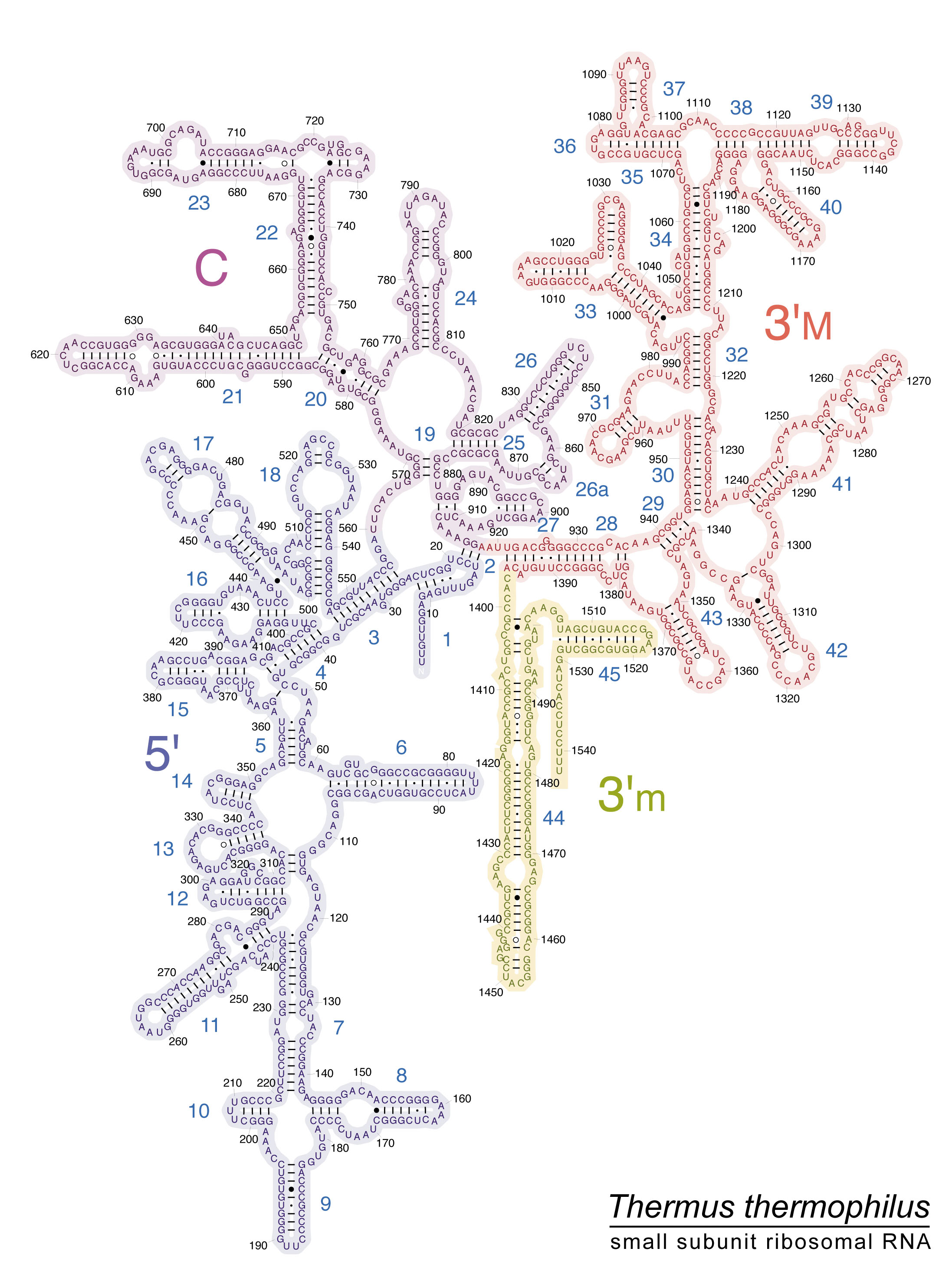
Four secondary structure properties are extracted from secondary structures, as shown as example for structural subelement h45 from the archaean Thermus thermophilus 16S rRNA (Fig. 2): 1. the percentage of nucleotides in stems formed by complementary self-hybridization among nucleotides, %stem among all nucleotides in the sequence; 2. the percentage of nucleotides, among those in loops, that are in loops topping stems (external loops), as opposed to unpaired nucleotides forming bulges within stems (internal loops), %eloops; and the 3. stem and 4. loop GC contents, in percentages.

Secondary structure of domain IV (ochre, structural subelements h44 and h45) and part of domain III (pink, structural subelement h43) of 16S rRNA of Thermus thermophilus (adapted from http://rna.ucsc.edu/rnacenter/images/figs/thermus_16s_2ndry.jpg). Boundaries between secondary structure subelements are from Fig. 2 in59. Subelement h44 ranges from nucleotides 1397 to 1505. Its only external loop is from nucleotides 1450 to 1454. Sixty nucleotides are involved in stems (G-U included, C-A, U-C and G-A excluded and considered as internal bulges). Hence, a total of 41 nucleotides are considered unpaired, including the external loop. %stem = 100 × 60/101 = 59.4; %eloop = 100 × 4/41 = 9.8; %GCstem = 100 × 52/60 = 86.7; and %GCloops = 100 × 22/41 = 53.7.
Similarities between two secondary structure pairs are estimated by Pearson correlation coefficients r between these four variables as obtained for each secondary structure (Fig. 3), in this case between values from Fig. 2 and those of secondary structures formed by two alternative splicings of RNA ring 25, also called AB53. Table 1 presents the four secondary structure variables for AB for all 22 alternative splicings of that RNA ring. Such data were obtained for all 25 RNA rings. Similar secondary structure data for 22 alternative splicings of RNA ring 13, called AL, were presented previously57, (therein Table 3). For each comparison, Fig. 3 has four datapoints for each secondary structure, one datapoint per secondary structure variable. For each datapoint, the X-axis is defined by the value obtained for the AB secondary structure, and the Y-axis by the value obtained for the corresponding variable for the 16S secondary structure subelement shown in Fig. 2. These pairings are not arbitrary: the x- and y-axis values are for the same secondary structure property, but for a different secondary structure (x-axis, RNA ring 25; y-axis, rRNA structural subelement, in this case h45 of Thermus thermophilus). Similarities are estimated by r, the more positive r, the more similar the secondary structures.

Similarity between secondary structure properties of structural subelement h45 of Thermus thermophilus 16S rRNA secondary structure and those of the secondary structure formed by AB (Table 1, secondary structures corresponding to splicing 7 and 19, filled and hollow symbols, respectively), as estimated by Pearson’s correlation coefficient r (note that r-squares are indicated in the figure). Each datapoint represents one of the four variables extracted from secondary structures, Y-axis values are from Fig. 2. Similarity with AB secondary structures, splicings 7 and 19, are: r = 0.633 and r = −0.979. The latter similarity is statistically significant at P < 0.05 (and indicates a stronger than random lack of similarity), the former indicates no similarity.
The secondary structure variables of all secondary structure subelements of two Archaea, Thermus thermophilus and Sulfolobus solfataricus104 (Table 2), two bacteria, Escherichia coli and Streptomyces coelicolor105 (Table 3), and the 18S rRNA of two eukaryotes, Homo sapiens and Saccharomyces cerevisiae (Table 4). Secondary rRNA structures for prokaryote 16S of Thermus thermophilus, Escherichia coli, and eukaryote 18S Saccharomyces cerevisiae and Homo sapiens are available at http://apollo.chemistry.gatech.edu/RibosomeGallery/.
Step by step description of analyses
-
1.
There are 25 RNA rings, each 22 nucleotide long. These are considered according to the splicing matching homology with ancestral tRNAs, as shown previously (Table 1 in50,57,100,102 and Table 2 in101).
-
2.
Each RNA ring can be spliced at 22 positions, and a different optimal secondary structure (predicted by Mfold103) exists for RNA ring sequences spliced at each potential splicing position. The 25 RNA rings form 25 × 22 = 550 secondary structures.
-
3.
Four secondary structure variables are extracted from each of these 550 secondary structures. Table 1 presents as an example these four variables for the 22 alternative splicings of a specific RNA ring, RNA ring 25.
-
4.
For each of the (about 45) structural subelements of small rRNA subunits of the 6 examined organisms, the four secondary structure variables are extracted, as was done for the 550 RNA ring structures at step 3. These variables are presented for the 6 × 45 = 270 secondary structure subelements presented in Tables 2–4.
-
5.
The secondary structures of RNA rings are compared to the secondary structures of rRNA structural subelements by analyses as presented in Fig. 3. These analyses plot the values obtained for each of the 4 secondary structure variables of a rRNA structural subelement as a function of the corresponding values obtained for a given RNA ring secondary structure. A Pearson correlation coefficient r, called rS, estimates similarities between rRNA and RNA ring secondary structures. Figure 3 presents comparisons between 16S rRNA subelement h45 of Thermus thermophilus and two RNA ring 25 secondary structures, one obtained by splicing that ring at position 7, and one at position 19.
For each of the 550 RNA ring secondary structures, there are as many rS as there are rRNA secondary structure subelements, about 45.
-
6.
According to our hypothesis, the (about) 45 rSs comparing a given RNA ring secondary structure to all rRNA structural subelements are potential estimates of the accretion order of the rRNA secondary structures.
-
7.
These rSs are compared to the accretion order of the rRNA secondary structure subelements, as these were determined by other methods and published by other authors (separately for each cladistic and structural accretion ranks). This comparison is done by calculating the Pearson correlation coefficient between the rS and the accretion orders, producing rH, one for the cladistic method, rHphyl, and one for the structural method, rHstru. Note that rS are z-transformed before calculating rH using the formula z = −ln((1 + r)/(1 − r)). The z transformation linearizes the scale of r, which is not linear.
-
8.
Hence, each of the 550 RNA ring secondary structures produces one rHphyl and one rHstru per organism. For each organism, there are 550 rHphyls and 550 rHstrus. The minimal and maximal rHphyls and rHstrus for each organism are in Table 5. Table 5 includes percentages of negative rHphyls and rHstrus (the working hypothesis expects negative rHs), and numbers of negative and positive rHphyls and rHstrus that have two tailed P < 0.05.
Table 5 Most negative and most positive Pearson correlations coefficients r (x100) (rH) between accretion ranks according to phylogenetic (rHphyl) and structural (rHstru) models with secondary structure similarities with RNA rings for 16S rRNAs of six organisms, and percentages of rHs (%neg) that are negative as expected by the working hypothesis among the 550 correlation calculated for each rHphyl and rHstru, for each organism. * indicates statistically significant differences (P < 0.05) from 50% (550/2 = 275 negative rHphyl and rHstru are expected if the sign of rH has an unbiased distribution between negative and positive trends) according to a chi-square test. “Co” indicates the cognate amino acid corresponding to the anticodon of the RNA ring(s) producing these correlations. Cognate G always corresponds to RNA ring 25 (AB). N indicates numbers of datapoints involved in the calculation of rH correlation coefficients. -
9.
For any given RNA ring secondary structure, there are 6 rHphyls and 6 rHstrus, because analyses were done for 6 organisms. There are in total 6 × 550 = 3300 rHphyls and 3300 rHstrus. Further analyses describe general patterns within these data, according to RNA rings, and according to splicing positions.
-
10.
For each RNA ring, there are 22 secondary structures which produce 22 rHphyls and 22 rHstrus per organism, hence 6 × 22 = 132 rHphyls and 132 rHstrus across all 6 organisms. An alternative way to explain this is: for each of the 25 RNA rings, there are 3300/22 = 132 rHphyls and 132 rHstrus across all 6 organisms.
Percentages of negative rHphyls and rHstrus for each RNA ring (calculated among the 132 rHphyls and among the 132 rHstrus, pooling all organisms) are used in the y axis of Fig. 4.
Figure 4 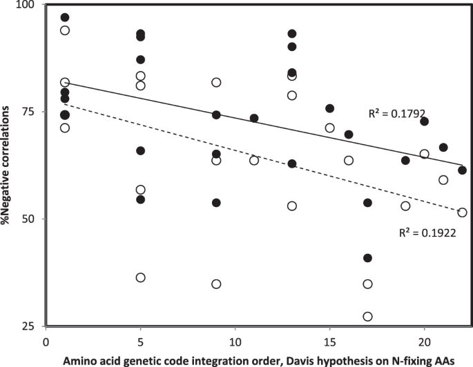
Percentage of negative Pearson correlation coefficients r between accretion ranks (phylogenetic method, filled symbols; structural method, hollow symbols) and similarities between 16S rRNA and RNA ring secondary structures, r’s pooled across organisms and secondary structures formed by the 22 alternative splicing of each RNA ring, as a function of the genetic code integration order of the RNA ring’s predicted cognate amino acid according to Davis’s hypothesis on N-fixing amino acids105. The working hypothesis expects negative r’s in particular for ancient amino acids.
-
11.
There are 25 RNA rings. Hence, for a given splicing position, there are 25 rHphyls and 25 rHstrus. Pooling these data across 6 organisms, for any given splicing position, there are 6 × 25 = 150 rHphyls and 150 rHstrus across all 6 organisms. Percentages of negative rHphyls and rHstrus for each splicing position, calculated from these 150 rHphyls and 150 rHstrus, consist the y axis in Fig. 5.
Figure 5 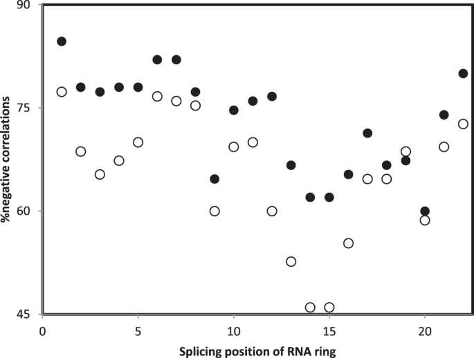
Percentage of negative Pearson correlation coefficient r between accretion ranks (phylogenetic method, filled symbols; structural method, hollow symbols) and similarities between 16S rRNA and RNA ring secondary structures, r’s pooled across organisms and RNA rings, as a function of the splicing position of the RNA ring. The splicing position with the highest percentage of negative correlations is position “1”, which corresponds to the splicing that produces the best homology between RNA rings and ancestral tRNAs57.


Analyses in Table 5, Figs. 4 and 5 each take into consideration all 3300 rHphyls and 3300 rHstrus. Hence, these are not biased representations of the data. They show separately effects of each ‘treatment factor’ (organism, RNA ring, splicing position) on each rHphyl and rHstru.
Results and discussion
There are 25 theoretical minimal RNA rings. Each has exactly 22 nucleotides, hence each RNA ring has 22 alternative splicing positions. Different splicings produce different sequences forming different secondary structures, as shown for RNA ring 25, AB, in Table 1, and previously for RNA rings 9106, (therein Table 1) and 1357, (therein Table 3). Hence, there are 25 × 22 = 550 secondary structures to which secondary structure subelements of the 16S rRNAs can be compared.
The secondary structure variables shown in Table 1 and Figs. 2 and 3 were extracted for each of these 550 RNA ring secondary structures and are compared, as shown in Fig. 3, with the corresponding secondary structure variables of all secondary structure subelements of all six organisms considered here.
Table 5 shows the most negative and the most positive rH correlations between secondary structure similarities and accretion ranks according to the phylogenetic and the structural method for each of the six organisms (rHphyl and rHstru, respectively). Similarities (rS) were between the secondary structure variables described in Tables 2–4 and corresponding variables for the secondary structures formed by each of the 22 alternative splicings of each of the 25 theoretical minimal RNA rings. Considering that the main prediction of the working hypothesis expects negative correlations, it is notable that in each organism, the absolute values of the negative correlation is larger than the absolute value of the positive correlation, besides for one among 12 comparisons, according to the structural method, for Sulfolobus solfataricus.
Similarly, percentages of negative correlations are in all organisms, for both rHphyl and rHstru, always greater than 50%, significantly so according to a chi-square test in all but three among 12 tests, rHphyl in Homo, rHstru in yeast and in Sulfolobus. In addition, percentages of negative rHs are significantly greater for rHphyl than rHstru within three among six species, Sulfolobus, Streptomyces and yeast. In Homo, percentages of negative rHstru were significantly greater than percentages of negative rHphyl. The overall pattern is that results match the working hypothesis, and this more for rHphyl than rHstru. The opposite occurs in Homo. This could be interpreted as due to recent evolution of small rRNA structure in that species, but would require additional analyses and data from other species.
A second noteworthy point is that the most positive correlations are in 7 among 12 cases with RNA ring 2, which has a predicted anticodon for a stop codon, coding sometimes for selenocysteine. This is presumably one of the latest amino acids integrated in the genetic code (21st). This result fits the prediction that the most positive correlations between accretion ranks and secondary structure similarities would correspond to RNA rings with recent cognates. In other words, these secondary structures would not be references for initial RNAs starting the accretion process, but for the latest RNAs in the accretion process.
Figure 4 plots percentages of negative r’s between accretion ranks and secondary structure similarities between small rRNA subelements and RNA ring secondary structures, pooling all organisms and alternative splicings of RNA rings. Patterns confirm several points: 1. Most correlations between accretion ranks and secondary structure similarities are negative as expected by the working hypothesis, for most RNA rings; 2. In most cases, there are more negative correlations for the phylogenetic than the structural method for reconstructing accretion ranks; 3. Percentages of negative correlations decrease with the genetic code integration order of the cognate amino acid of RNA rings (see above comments for RNA ring with selenocysteine as predicted cognate).
Figure 5 presents the percentages of negative r’s between accretion ranks and secondary structure similarities between small rRNA subelements and RNA ring secondary structures, pooling all organisms and RNA rings, as a function of RNA ring splicing position. Results show that correlations are most frequently negative, meaning fitting the working hypothesis, when RNA rings are spliced at position “1”. This is the position defined by the highest homology between the RNA ring and an ancestral tRNA55. This observation is also in line with the working hypothesis that RNA rings are proto-tRNAs, and that accretion of proto-tRNAs, tRNAs and tRNA-like RNAs formed rRNAs. Note that the assumption that RNA rings are proto-tRNAs is under debate107. Nevertheless, and apparently confirming this status of proto-tRNAs, pseudo-phylogenetic analyses of RNA ring sequences reveal two clusters of RNA rings, one coinciding with RNA rings whose presumed cognate amino acid is the cognate of tRNAs for which the tRNA acceptor stem includes a primitive code108.
Particularly noteworthy is that results of analyses presented here for the small rRNA subunit are in line with results obtained for the large rRNA subunit106. These analyses compared structural subelements of the large rRNA subunit with the same RNA ring secondary structures as those used here. As described here for the small rRNA, for the large rRNA subunit, comparisons with RNA ring secondary structures show that: a. are slightly more congruent with the phylogenetic than the structural method; b. results are strongest for comparisons with RNA rings with predicted ancient cognate amino acids; c. weakest for comparisons with RNA rings with predicted recent cognate amino acids.
Conclusions
Results are strong corroboration of the working hypothesis that tRNA accretions formed rRNAs. They show that RNA rings are likely proto-tRNAs, and that these are good reference points for primitive RNAs in general, and tRNAs in particular. Results confirm that RNA ring cognates are good estimates for RNA ring evolutionary ranks, and that similarities between secondary structures bear information on evolutionary direction of RNA secondary structures, from tRNA to rRNA-like, also among rRNA structural subelements. This has been suggested by several previous lines of analyses presented in the Introduction10,11,12,15,16,17,18,19,20,21,56,57,91,92, expanding upon evidences for common origins for tRNAs and rRNAs1,2,3,4,7,8,9. Analyses presented here for the small rRNA subunit show greater congruence between accretion orders derived from the secondary structure method used here and the phylogenetic method than between the former and the structural method. Similar analyses done for the large rRNA subunit produce qualitatively similar results, independently confirming our method and evolutionary conclusions. Overall, both phylogenetic and structural methods produce accretion orders that are congruent with the secondary structure method applied through the tRNA-rRNA axis of RNA secondary structure evolution. It is probable that the structural methods are more prone to errors due to evolutionary convergences than the phylogenetic method, though convergences remain the main difficulty in reconstructing evolution.
References
Bloch, D. P. et al. tRNA-rRNA sequence homologies: evidence for a common evolutionary origin? J. Mol. Evol. 19, 420–428 (1983).
Bloch, D. P. et al. tRNA-rRNA sequence homologies: a model for the origin of a common ancestral molecule, and prospects for its reconstruction. Orig. Life Biosph. 14, 571–578 (1984).
Bloch, D. P., McArthur, B. & Mirrop, S. RNA-rRNA sequence homologies: evidence for an ancient modular format shared by tRNAs and rRNAs. Biosystems 17, 209–225 (1985).
Bloch, D. P., McArthur, B., Guimaraes, R. C., Smith, J. & Staves, M. P. tRNA-rRNA sequence matches from inter- and intraspecies comparisons suggest common origins for the two RNAs. Braz. J. Med. Biol. Res. 22, 931–944 (1989).
Caetano-Anollés, G. Tracing the evolution of RNA structure in ribosomes. Nuc. Acids Res. 30, 2575–2587 (2002).
Caetano-Anollés, G. & Sun, F. J. The natural history of transfer RNA and its interactions with the ribosome. Front. Genet. 5, 127 (2014).
Root-Bernstein, M. & Root-Bernstein, R. The ribosome as a missing link in the evolution of life. J. Theor. Biol. 367, 130–158 (2015).
Root-Bernstein, R. & Root-Bernstein, M. The ribosome as a missing link in prebiotic evolution II: Ribosomes encode ribosomal proteins that bind to common regions of their own mRNAs and rRNAs. J. Theor. Biol. 397, 115–127 (2014).
Barthélémy, R. M. & Seligmann, H. Cryptic tRNAs in chaetognath mitochondrial genomes. Comput. Biol. Chem. 62, 119–132 (2016).
Caetano-Anollés, D. & Caetano-Anollés, G. Piecemeal buildup of the genetic code, ribosomes, and genomes from primordial tRNA building blocks. Life (Basel) 6, e43 (2016).
Farias, S. T., Rêgo, T. G. & José, M. V. Origin of the 16S ribosomal molecule from ancestor tRNAs. Sci. 1, 8 (2019).
Agmon, I. The dimeric proto-ribosome: structural details and possible implications on the origin of life. Int. J. Mol. Sci. 10, 2921–2934 (2009).
Farias, S. T., Rêgo, T. G. & José, M. V. Origin and evolution of the peptidyl transferase center from proto-tRNAs. FEBS Open Bio. 4, 175–178 (2014).
Agmon, I. C. Could a proto-ribosome emerge spontaneously in the prebiotic world? Molecules 21, e1701 (2016).
Guimaraes, R. C., Moreira, C. H. & de Farias, S. T. A self-referential model for the formation of the genetic code. Theory Biosci. 127, 249–270 (2008).
Guimaraes, R. C. Metabolic basis for the self-referential genetic code. Orig. Life Evol. Biosph. 41, 357–371 (2011).
Guimaraes, R. C. Essentials in the life process indicated by the self-referential genetic code. Orig. Life Evol. Biosph. 44, 269–277 (2014).
Guimaraes, R. C. The self-referential genetic code is biologic and includes the error minimization property. Orig. Life Evol. Biosph. 45, 69–75 (2015).
Guimaraes, C. R. Self-referential encoding on modules of anticodon pairs-roots of the biological flow system. Life (Basel) 7, e16 (2017).
Brown, A. et al. Structure of the large ribosomal subunit from human mitochondria. Science 346, 718–722 (2014).
Amunts, A., Brown, A., Toots, J., Scheres, S. H. W. & Ramakrishnan, V. Ribosome. The structure of the human mitochondrial ribosome. Science 348, 95–98 (2015).
Di Giulio, M. Was it an ancient gene codifying for a hairpin RNA that, by means of direct duplication, gave rise to the primitive tRNA molecule? J. Theor. Biol. 177, 95–101 (1995).
Di Giulio, M. The non-monophyletic origin of the tRNA molecule. J. Theor. Biol. 197, 403–414 (1999).
Di Giulio, M. The non-monophyletic origin of the tRNA molecule and the origin of genes only after the evolutionary stage of the last universal common ancestor (LUCA). J. Theor. Biol. 240, 343–352 (2006a).
Seligmann, H. & Amzallag, G. N. Chemical interactions between amino acid and RNA: multiplicity of the levels of specificity explains origin of the genetic code. Naturwissenschaften 89, 542–551 (2002).
Di Giulio, M. Permuted tRNA genes of Cyanidioschyzon merolae, the origin of the tRNA molecule and the root of the Eukarya domain. J. Theor. Biol. 253, 587–592 (2006b).
Di Giulio, M. The split genes of Nanoarchaeum equitans are an ancestral character. Gene 421, 20–26 (2008).
Di Giulio, M. Transfer RNA genes in pieces are an ancestral character. EMBO Rep. 9, 820 (2008).
Di Giulio, M. A comparison among the models proposed to explain the origin of the tRNA molecule: A synthesis. J. Mol. Evol. 69, 1–9 (2009).
Di Giulio, M. Formal proof that the split genes of tRNAs of Nanoarchaeum equitans are an ancestral character. J. Theor. Biol. 266, 569–572 (2009b).
Di Giulio, M. The origin of the tRNA molecule: Independent data favor a specific model of its evolution. Biochimie 94, 1464–1466 (2012).
Di Giulio, M. The ‘recently’ split transfer RNA genes may be close to merging the two halves of the tRNA rather than having just separated them. J. Theor. Biol. 310, 1–2 (2012).
Di Giulio, M. A polyphyletic model for the origin of tRNAs has more support than a monophyletic model. J. Theor. Biol. 318, 124–128 (2013).
Di Giulio, M. The split genes of Nanoarchaeum equitans have not originated in its lineage and have been merged in another Nanoarchaeota: a reply to Podar et al. J. Theor. Biol. 349, 167–169 (2014).
Widmann, J., Di Giulio, M., Yarus, M. & Knight, R. tRNA creation by hairpin duplication. J. Mol. Evol. 61, 524–530 (2005).
Branciamore, S. & Di Giulio, M. The presence in tRNA molecule sequences of the double hairpin, an evolutionary stage through which the origin of this molecule is thought to have passed. J. Mol. Evol. 72, 652–363 (2011).
Fujishima, K. et al. A novel three-unit tRNA splicing endonuclease found in ultrasmall Archaea possesses broad substrate specificity. Nuc. Acids Res. 39, 9695–9704 (2011).
Seligmann, H. Pocketknife tRNA hypothesis: anticodons in mammal mitochondrial tRNA side-arm loops translate proteins? Biosystems 113, 165–76 (2013a).
Seligmann, H. Putative anticodons in mitochondrial tRNA sidearm loops: Pocketknife tRNAs? J. Theor. Biol. 340, 155–163 (2014a).
Faure, E., Barthélémy, R.M. True tRNA punctuation and initiation using overlapping stop and start codons at specific and conserved positions. Mitochondrial DNA – New insights (eds. Seligmann, H., Warthi, G.). IntechOpen, London, https://doi.org/10.5772/intechopen.75555 (2018).
Faure, E. & Barthélémy, R. M. Specific mitochondrial ss-tRNAs in phylum Chaetognatha. J. Entomol. Zool. Studies 7, 304–315 (2019).
Branciamore, S. & Di Giulio, M. The origin of the 5s ribosomal RNA molecule could have been caused by a single inverse duplication: strong evidence from its sequences. J. Mol. Evol. 74, 170–186 (2012).
Maizels, N. & Weiner, A. M. Phylogeny from function: evidence from the molecular fossil record that tRNA originated in replication, not translation. Proc. Natl. Acad. Sci. USA 91, 6729–6734 (1995).
Seligmann, H. & Krishnan, N. M. Mitochondrial replication origin stability and propensity of adjacent tRNA genes to form putative replication origins increase developmental stability in lizards. J. Exp. Zool. B Mol. Dev. Evol. 306, 433–449 (2006).
Seligmann, H. & Labra, A. The relation between hairpin formation by mitochondrial WANCY tRNAs and the occurrence of the light strand replication origin in Lepidosauria. Gene 542, 248–257 (2014).
Seligmann, H. Hybridization between mitochondrial heavy strand tDNA and expressed light strand tRNA modulates the function of heavy strand tDNA as light strand replication origin. J. Mol. Biol. 379, 188–199 (2008).
Seligmann, H. Mitochondrial tRNAs as light strand replication origins: similarity between anticodon loops and the loop of the light strand replication origin predicts initiation of DNA replication. Biosystems 99, 85–93 (2010a).
Seligmann, H. Mutation patterns due to converging mitochondrial replication and transcription increase lifespan, and cause growth rate-longevity tradeoffs. DNA Replication – Current Advances (ed. Seligmann, H.), Chapter 6, InTechOpen, London, ISBN 978-953-307-593-8 (2011).
Seligmann, H. & Swinger, R. N. A. self-hybridization and mitochondrial non-canonical swinger transcription, transcription systematically exchanging nucleotides. J. Theor. Biol. 399, 84–91 (2016).
Demongeot, J. & Seligmann, H. Theoretical minimal RNA rings designed according to coding constraints mimic deamination gradients. Naturwissenschaften 106, 44 (2019a).
Michel, C. J. Circular code motifs in transfer and 16S ribosomal RNAs: a possible translation code in genes. Comput. Biol. Chem. 37, 24–37 (2012).
Michel, C. J. Circular code motifs in transfer RNAs. Comput. Biol. Chem. 45, 17–29 (2013).
Demongeot, J. Sur la possibilité de considérer le code génétique comme un code à enchaînement. Revue de Biomaths 62, 61–66 (1978).
Demongeot, J. & Besson, J. Genetic-code and cyclic codes. Comptes R. Acad. Sci. III Life Sci. 296, 807–810 (1983).
Demongeot, J. & Moreira, A. A possible circular RNA at the origin of life. J. Theor. Biol. 249, 314–324 (2007).
Demongeot, J., Seligmann, H. Evolution of tRNA into rRNA secondary structures. Gene Rep., in press (2019b).
Demongeot, J., Seligmann, H. The Uroboros theory of life’s origin: 22-nucleotide theoretical minimal RNA rings reflect evolution of genetic code and tRNA-rRNA translation machineries. Acta Biotheoretica, in press (2019c).
Caetano-Anollés, K., Caetano-Anollés, D., Nasir, A., Kim, K. M. & Caetano-Anollés, G. Order and polarity in character state transformation models that root the tree of life. Biochimie 149, 135–136 (2018).
Harish, A. & Caetano-Anollés, G. Ribosomal history reveals origins of modern protein synthesis. PLoS One 7, e32776 (2012).
Stewart, C. B. The powers and pitfalls of parsimony. Nature 361, 603–607 (1993).
Kim, K. M., Nasir, A., Hwang, K. & Caetano-Anollés, G. A tree of cellular life inferred from a genomic census of molecular functions. J. Mol. Evol. 79, 240–262 (2014).
Nasir, A., Kim, K. M. & Caetano-Anollés, G. A phylogenomic census of molecular functions identifies modern thermophilic archaea as the most ancient form of cellular life. Archaea 2014, 706468 (2014).
Caetano-Anollés, G., Mittenthal, J. E., Caetano-Anollés, D. & Kim, K. M. A calibrated chronology of biochemistry reveals a stem line of descent responsible for planetary biodiversity. Front. Genet. 5, 306 (2014).
Nasir, A., Kim, K. M. & Caetano-Anollés, G. Phylogenetic tracings of proteome size support the gradual accretion of protein structural domains and the early origin of viruses from primordial cells. Front. Microbiol. 8, 1178 (2017).
Hillis, D. M., Bull, J. J., White, M. E., Badgett, M. R. & Molineux, I. J. Experimental phylogenetics—generation of a known phylogeny. Science 264, 671–677 (1992).
Hillis, D. M., Huelsenbeck, J. P. & Cunningham, C. W. Application and accuracy of molecular phylogenies. Science 264, 671–677 (1994).
Leitner, T., Escanilla, D., Franzén, C., Uhlén, M. & Albert, J. Accurate reconstruction of a known HIV-1 transmission history by phylogenetic tree analysis. Proc. Natl. Acad. Sci. USA 93, 10864–10869 (1996).
Cunningham, C. W., Zhu, H. & Hillis, D. M. Best-fit maximum-likelihood models for phylogenetic inference: empirical tests with known phylogenies. Evolution 52, 979–987 (1998).
Polly, P. D. Paleontology and the comparative method: ancestral node reconstructions versus observed node values. Am. Nat. 157, 596–609 (2001).
Webster, A. J. & Purvis, A. Testing the accuracy of methods for reconstructing ancestral states of continuous characters. Proc. Biol. Sci. 269, 143–149 (2002).
Krishnan, N. M., Seligmann, H., Stewart, C. B., de Koning, A. P. & Pollock, D. D. Ancestral sequence reconstruction in primate mitochondrial DNA: Compositional bias and effect on functional inference. Mol. Biol. Evol. 21, 1871–1883 (2004).
Spencer, M., Davidson, E. A., Barbrook, A. C. & Howe, C. J. Phylogenetics of artificial manuscripts. J. Theor. Biol. 227, 503–511 (2004).
Raaum, R. L., Sterner, K. N., Noviello, C. M., Stewart, C. B. & Disotell, T. R. Catarrhine primate divergence dates estimated from complete mitochondrial genomes: concordance with fossil and nuclear DNA evidence. J. Hum. Evol. 48, 237–257 (2005).
Finarelli, J. A. & Flynn, J. J. Ancestral state reconstruction of body size in the Caniformia (Carnivora, Mammalia): the effects of incorporating data from the fossil record. Syst. Biol. 55, 301–3013 (2006).
Seligmann, H. Positive correlations between molecular and morphological rates of evolution. J. Theor. Biol. 264, 799–807 (2010b).
Hsiao, C., Mohan, S., Kalahar, B. K. & Williams, L. D. Peeling the onion: ribosomes are ancient molecular fossils. Mol. Biol. Evol. 26, 2415–2425 (2009).
Lanier, K. A., Athavale, S. S., Petrov, A. S., Wartell, R. & Williams, L. D. Imprint of ancient evolution on rRNA folding. Biochemistry 55, 4603–4613 (2016).
Petrov, A. S. et al. History of the ribosome and the origin of translation. Proc. Natl. Acad. Sci. USA 112, 15396–15401 (2015).
Johnson, D. B. F. & Wang, L. Imprints of the genetic code in the ribosome. Proc. Natl. Acad. Sci. USA 107, 8298–8303 (2010).
Lifson, S. Chemical selection, diversity, teleonomy and the second law of thermodynamics. Reflections on Eigen’s theory of self-organization of matter. Biophys. Chem. 26, 303–311 (1987).
Seligmann, H. Protein sequences recapitulate genetic code evolution. Comput. Struct. Biotechnol. J. 16, 177–189 (2018).
Lovtrup, S. O. von Baerian and Haeckelian recapitulation. Syst. Zool. 27, 348–352 (1978).
Kalinka, A. T. & Tomancak, P. The evolution of early animal embryos: conservation or divergence. Trends Ecol. Evol. 27, 385–393 (2012).
Seligmann, H. Resource partition history and evolutionary specialization of subunits in complex systems. Biosystems 51, 31–39 (1999).
Horn, H. S. Forest succession. Sci. American 232, 90–101 (1975).
Wardle, P. Primary succession in Westland National park and its vicinity, New Zealand. New Zealand J. Bot. 18, 221–232 (1980).
Caetano-Anollés, G. Ancestral insertions and expansions of rRNA do not support an origin of the ribosome in its peptidyl transferase center. J. Mol. Evol. 80, 162–165 (2015).
Caetano-Anollés, G. & Caetano-Anollés, D. Computing the origin and evolution of the ribosome from its structure - Uncovering processes of macromolecular accretion benefiting synthetic biology. Comput. Struct. Biotechnol. J. 13, 427–447 (2015).
Caetano-Anollés, G. & Caetano-Anollés, D. Commentary: History of the ribosome and the origin of translation. Front. Mol. Biosci. 3, 87 (2017).
Seligmann, H. Evolution and ecology of developmental processes and of the resulting morphology: directional asymmetry in hindlimbs of Agamidae and Lacertidae (Reptilia: Lacertilia). Biol. J. Linn. Soc. 69, 461–481 (2000).
Seligmann, H. & Raoult, D. Unifying view of stem-loop hairpin RNA as origin of current and ancient parasitic and non-parasitic RNAs, including in giant viruses. Curr. Opin. Microbiol. 31, 1–8 (2016).
Seligmann, H., Raoult, D. & Stem-loop, R. N. A. hairpins in giant viruses: invading rRNA-like repeats and a template free. RNA. Front. Microbiol. 9, 101 (2018).
Chaley, M.B., Korotkov, E.V. and Phoenix, D.A. Relationships among isoacceptor tRNAs seems to support the coevolution theory of the origin of the genetic code. J. Mol. Evol. 48, 168-177.
Trifonov, E. N. Consensus temporal order of amino acids and evolution of the triplet code. Gene 264, 139–151 (2000).
Sun, F. J. & Caetano-Anollés, G. The origin of modern 5S rRNA: a case of relating models of structural history to phylogenetic data. J. Mol. Evol. 71, 3–5 (2010).
Bokov, K. & Steinberg, S. V. A hierarchical model for evolution of 23S ribosomal RNA. Nature 457, 977–980 (2009).
Eigen, M. & Winkler-Oswatitsch, R. Transfer-RNA: the early adaptor. Naturwissenschaften 68, 217–228 (1981a).
Eigen, M. & Winkler-Oswatitsch, R. Transfer-RNA, an early gene? Naturwissenschaften 68, 282–292 (1981b).
Demongeot, J. & Seligmann, H. Theoretical minimal RNA rings recapitulate the order of the genetic code’s codon-amino acid assignments. J. Theor. Biol. 471, 108–116 (2019d).
Demongeot, J. & Seligmann, H. Bias for 3’-dominant codon directional asymmetry in theoretical minimal RNA rings. J Comput Biol. 26, 1003–1012 (2019e).
Demongeot, J. & Seligmann, H. Spontaneous evolution of circular codes in theoretical minimal RNA rings. Gene 705, 95–102 (2019f).
Demongeot, J. & Seligmann, H. More pieces of ancient than recent theoretical minimal proto-tRNA-like RNA rings in genes coding for tRNA synthetases. J. Mol. Evol. 87, 152–174 (2019g).
Zuker, M. Mfold web server for nucleic acid folding and hybridization prediction. Nucleic Acids Res. 31, 3406–3415 (2003).
Olsen, G. J. et al. Sequence of the 16S rRNA gene from the thermoacidophilic archaebacterium Sulfolobus solfataricus and its evolutionary implications. J. Mol. Evol. 22, 301–307 (1985).
Anderson, A. S. & Wellington, E. M. The taxonomy of Streptomyces and related genera. Int. J. Syst. Evol. Microbiol. 51, 797–814 (2001).
Demongeot, J., Seligmann, H. Accretion history of large ribosomal subunits deduced from theoretical minimal RNA rings is congruent with histories derived from phylogenetic and structural methods. Gene 734, https://doi.org/10.1016/j.gene.2020.144436 (2020a).
Demongeot, J., Seligmann, H. RNA rings strengthen hairpin accretion hypotheses for tRNA evolution: a reply to commentaries by Z.F. Burton and M. Di Giulio. J. Mol. Evol. 88, https://doi.org/10.1007/s00239-020-09929-1 (2020b).
Demongeot, J. & Seligmann, H. The primordial tRNA acceptor stem code from theoretical minimal RNA ring clusters. BMC Genetics 21, 7 (2020c).
Weiner, A. M. & Maizels, N. tRNA-like structures tag the 3′ ends of genomic RNA molecules for replication: implications for the origin of protein synthesis. Proc. Natl. Acad. Sci. USA. 84, 7383–7387 (1987).
Gulen, B., et al. Ribosomal small subunit domains radiate from a central core. Sci. Rep. 6, 20885 (2016).
Davis, B. K. Evolution of the genetic code. Prog. Biophys. Mol. Biol. 72, 157–243 (1999).
Author information
Authors and Affiliations
Contributions
J.D. and H.S. wrote the main manuscript text. All authors reviewed the manuscript.
Corresponding author
Ethics declarations
Competing interests
The authors declare no competing interests.
Additional information
Publisher’s note Springer Nature remains neutral with regard to jurisdictional claims in published maps and institutional affiliations.
Rights and permissions
Open Access This article is licensed under a Creative Commons Attribution 4.0 International License, which permits use, sharing, adaptation, distribution and reproduction in any medium or format, as long as you give appropriate credit to the original author(s) and the source, provide a link to the Creative Commons license, and indicate if changes were made. The images or other third party material in this article are included in the article’s Creative Commons license, unless indicated otherwise in a credit line to the material. If material is not included in the article’s Creative Commons license and your intended use is not permitted by statutory regulation or exceeds the permitted use, you will need to obtain permission directly from the copyright holder. To view a copy of this license, visit http://creativecommons.org/licenses/by/4.0/.
About this article

Cite this article
Demongeot, J., Seligmann, H. Comparisons between small ribosomal RNA and theoretical minimal RNA ring secondary structures confirm phylogenetic and structural accretion histories. Sci Rep 10, 7693 (2020). https://doi.org/10.1038/s41598-020-64627-8
Received:
Accepted:
Published:
DOI: https://doi.org/10.1038/s41598-020-64627-8
This article is cited by
-
On Protein Loops, Prior Molecular States and Common Ancestors of Life
Journal of Molecular Evolution (2024)
-
Origin of the 16S Ribosomal Molecule from Ancestor tRNAs
Journal of Molecular Evolution (2021)
-
Structural modeling and phylogenetic analysis for infectious disease transmission pattern based on maximum likelihood tree approach
Journal of Ambient Intelligence and Humanized Computing (2021)
-
First arrived, first served: competition between codons for codon-amino acid stereochemical interactions determined early genetic code assignments
The Science of Nature (2020)
Comments
By submitting a comment you agree to abide by our Terms and Community Guidelines. If you find something abusive or that does not comply with our terms or guidelines please flag it as inappropriate.
