
Abstract
We present a dataset of reconstructed three-dimensional (3D) englacial stratigraphic horizons in northern Greenland. The data cover four different regions representing key ice-dynamic settings in Greenland: (i) the onset of Petermann Glacier, (ii) a region upstream of the 79° North Glacier (Nioghalvfjerdsbræ), near the northern Greenland ice divide, (iii) the onset of the Northeast Greenland Ice Stream (NEGIS) and (iv) a 700 km wide region extending across the central ice divide over the entire northern part of central Greenland. In this paper, we promote the advantages of a 3D perspective of deformed englacial stratigraphy and explain how 3D horizons provide an improved basis for interpreting and reconstructing the ice-dynamic history. The 3D horizons are provided in various formats to allow a wide range of applications and reproducibility of results.
Background & Summary
Over the last decades, the Arctic, and thus, the Greenland ice sheet (GrIS), has warmed more intensively than other regions1,2. The resulting trend in mass loss of the GrIS contributes to sea-level rise of approximately 0.8 mm/a3. Approximately half of the mass loss is attributed to the ice-dynamical contribution from the acceleration of GrIS’ marine-terminating glaciers4,5. However, in contrast to the ice-mass loss driven by melting, the projected contributions to sea-level rise due to ice dynamics are associated with high uncertainties6. Over the last decade, critical regions in the GrIS experienced extensive speedup and thinning due to frontal ice retreat, affecting the inland ice-flow dynamics7. To better predict future dynamic mass losses, studying past ice-dynamical processes can provide important insight and constraints on forward ice-flow modelling.
The GrIS has been extensively mapped with radio-echo sounding (RES) surveys to quantify the thickness of the ice and to map the englacial stratigraphy8,9,10,11. The transmitted electromagnetic waves from the RES system get reflected at interfaces of dielectric contrasts12 within the ice column at so-called internal reflection horizons (IRHs). In the shallow and middle section of the ice column, IRHs primarily represent paleo surfaces that are caused by the former deposition of volcanic material13 at the surface and subsequently buried by subsequent snow accumulation, and hence, represent a horizon of a consistent time of deposition14. These IRHs provide a detailed insight into the englacial stratigraphy8,15,16,17,18.
Viewing the englacial stratigraphy of IRHs at high spatial resolution and in three dimensions has spatial advantages, potentially allowing better process understanding within and at the boundaries of the ice sheet, such as deformation, accumulation, melting and freezing. Three-dimensional views of IRHs within the ice sheets are obtained by tracing IRHs along RES profiles and then interpolating surfaces of equal age between different profiles, allowing the reconstruction of the 3D character of IRHs19 (which we will refer to as 3D horizons). This way, many of the processes occurring in the past, such as changes in the flow and melting of ice sheets, are preserved in the ice and can be decoded20,21,22,23,24,25.
This paper describes the publication of 3D horizons in the Greenland ice sheet. The horizons reflect the deformation history in different ice-dynamic regimes. A previous study has shown that 3D horizons can provide a holistic overview of the spatial variations in the character of the ice, such as deciphering folding processes due to the mechanical anisotropy of ice at the onset of ice streams19. Furthermore, 3D horizons revealed the past activity of paleo-ice streams in currently slow-flowing regions in northern central Greenland21. In addition to the publication of the data in various file formats, we explain in detail how and on what basis the 3D horizons were generated. The datasets are archived and available in a Pangaea Publication Series: https://doi.org/10.1594/PANGAEA.95499126.
Methods
Study regions
The data presented in this study originate from four different regions in northern Greenland (Fig. 1) that represent different regional glaciological and ice-dynamic settings: (i) the onset region of fast ice flow of the Petermann Glacier (Petermann Gletsjer), (ii) a region upstream of the 79° North Glacier (Nioghalvfjerdsbræ) in the vicinity of the ice divide (FINEGIS; Folds in the northeast Greenland ice sheet), (iii) the upstream region of the Northeast Greenland Ice Stream (NEGIS), and (iv) a large area covering Northern Central Greenland from the west over the central ice divide to the east.

Overview of the locations of the four data sets of 3D englacial stratigraphy horizons in northern Greenland: Petermann (orange), FINEGIS (Folds in the Northeast Greenland ice sheet; blue), NEGIS (Northeast Greenland Ice Stream onset; green) and Northern Central Greenland (violet). The base map shows the bed topography47 overlain with a colour map of the ice surface velocity85 of Greenland. The map has a vertical exaggeration of 15, and the ice surface velocity is shown on a logarithmic scale.
Petermann glacier
The first data set presented here covers the onset of the Petermann Glacier (PG). PG is located in northwest Greenland and represents one of Greenland’s largest outlet glaciers, draining about 4% of the GrIS27. The ice shelf of the PG is confined by a fjord and represents the longest floating tongue in Greenland28. Recent calving events in 2010 and 201229 have substantially shortened the ice shelf, which caused an average ice-flow acceleration of ∼10% between 2012 and 201730. Further concerns have been raised that subsequent future ice shelf loss might lead to speedup of the grounded part of PG, leading to irreversible grounding line retreat and accelerated mass loss30,31,32,33.
The upstream regions of fast flow are not topographically confined by a trough34. The basal conditions at the onset of the PG show a complex thermal transition at the base near the onset of fast ice flow35. Moreover, PG’s fast flow onset region is associated with folded and discontinuous IRHs buried deep in the ice sheet19, 36,37,38. The folding of the stratigraphy at PG’s onset has been attributed to various processes: Several studies point to basal conditions in the form of moving patches of subglacial slip39 and basal freeze-on36. By contrast, Bons et al.19 used the complete and extensive grid of NASA’s Operation IceBridge (OIB) RES profiles11 to construct 3D horizons, thus overcoming the limitations of using the interpretation on individual RES profiles only, as done in the previous two studies36,39. For the first time, this revealed the entire 3D geometry and orientation of the englacial folds (Fig. 2). Using the orientation of the fold axes, the authors concluded that converging flow and the mechanical anisotropy of the ice sufficiently explained the large-scale folding at the onset of the PG and no spatial variations in physical properties at the base need to be taken into account.

Folded IRH observed from different perspectives in RES data. (a) Overview map showing the P1 Petermann horizon and four RES profiles at different orientations (b–e). The y-axis (Elevation) of the radargrams is relative to the WGS84 ellipsoid, and the orange line in the radargrams (b-e) represents the IRH of the P1 3D horizon schematically.
Folds in the northeast greenland ice sheet (FINEGIS)
The second data set is located in northeast Greenland in the upstream part of the northern catchment of the 79° North Glacier. The region extends approximately from 79°N to 80°N and from 32°W to 40°W (FINEGIS in Fig. 1). Ice surface velocity in this region is almost zero in the western part as it is located close to Greenland’s central ice divide. Further east, ice flow velocity increases up to 15 ma−1. Two cylindrical fold units in this area are partly intersected by OIB RES profiles and have been subject to prior studies37,38,40. A systematic structural analysis of these folds based on additional high-resolution RES data allowed the creation of 3D horizons of the folded englacial stratigraphy. The geometry and deformation patterns of the folds were attributed to the time-varying activity of a now-extinct ice stream that first changed the flow pattern in its catchment and then was deactivated in the Holocene21. Locally this ancient ice-flow regime must have been much more focused and reached further inland than today.
Northeast Greenland Ice Stream onset region
The third data set covers the upstream part of the Northeast Greenland Ice Stream (NEGIS). Its onset region is close to the central divide, more than 500 km inland from its outlets (Fig. 1). In the course of predicting the future behaviour of the GrIS, the NEGIS represents one of the largest uncertainties for ice flow predictions41. Near its outlets42 (Zachariæ Isstrøm and Storstrømmen Glacier; Fig. 1), NEGIS is increasingly losing mass over the last decades43, mainly due to the retreat of the grounding line of NEGIS’ outlet glaciers (e.g., the rapid retreat of Zachariae Isstrom44). The resulting thinning and flow acceleration has the potential to propagate upstream45. Acceleration rates in the order of a few cma−1 at EastGRIP (East Greenland Ice-core Project)7,46 are first indications that the whole of NEGIS may not be in equilibrium.
Apart from its exceptional length in the Greenlandic context, NEGIS is also unique regarding its distinct and continuous shear margins along its entire length. The position of these shear margins appears not to be constrained by the underlying bed topography47,48. However, the geometry of the ice stream, the position of its shear margins, and the origin of NEGIS itself are still not fully understood21,49,50,51,52,53,54. Progress in this field is expected from analyzing the EastGRIP ice core55,56, GPS measurements46,57, an extensive grid of RES profiles flown over NEGIS58,59, ground-based phase sensitive RES (pRES) measurements60,61, and modelling62,63,64.
Northern central greenland
The fourth data set covers a ∼700 km wide strip extending across the central ice divide over the entire northern part of central Greenland (Fig. 1). In the east, the data set extends into the shear margin of NEGIS at its downstream end; in the west, into the region of elevated flow velocity of the northwest Greenland outlet glaciers. Characteristic features that the dataset covers in the central area and that define the local radio-stratigraphy are, for example, the englacial imprint in the stratigraphy of a paleofluvial mega-canyon in the bed topography65 and numerous plume-like folds, which were attributed to basal freeze-on processes38.
The perspective of 3D englacial stratigraphy
The way the geometry of IRHs imaged in radargrams is perceived depends on the orientation of the RES profile in relation to the three-dimensional geometry of the englacial stratigraphy — in short, the cutting angle. For example, cylindrical folds, such as those at Petermann Glacier19, appear very different depending on the orientation of the RES profile (Fig. 2). The geometries of the folds change depending on the angle of incision and appear misleading if viewed at angles other than 90° to the orientation of the fold axis (Fig. 2b,d). The greater the deviation from this orientation, the longer the wavelength of these folds appears (Fig. 2c,e). These distorted geometries can lead to significant misunderstandings and misinterpretations of processes involved in the formation of folds. Three-dimensional reconstruction provides remedy. We, therefore, consider it essential, especially for understanding the formation processes over time and spatial classification of deformations of the englacial stratigraphy19,21.
Workflow
The construction of 3D horizons begins with RES data acquisition over the ice sheet. Several steps are necessary before the full 3D product is produced, which are presented in this section. A schematic overview of the steps is shown in Fig. 3.

Workflow sequence for 3D horizon construction from RES data acquisition to the scientific analysis of 3D horizons.
Data sources and data acquisition
The basis for generating the data products published here is airborne RES data. The RES data used to create the 3D horizons presented here were acquired with multi-channel coherent depths sounders (MCoRDS) flown by the Center for Remote Sensing and Integrated Systems (CReSIS) and NASA’s Operation IceBridge11,66 as well as surveys from the Alfred Wegener Institute, Helmholtz Centre for Polar and Marine Research (AWI)21,58,67 with AWI’s polar research aircrafts68. The radar specifications for the RES data used in each of the four survey regions are shown in Table 1. A complete list with all RES profiles used for the reconstruction of the 3D horizons is shown in Table 2.
Radio-echo sounding data processing
The RES data processing for all MCoRDS systems was performed with the CReSIS Toolbox69 and consisted of four main steps: (1) GPS synchronization, (2) pulse compression of the chirped waveform in the vertical range to improve the range signal quality and the signal-to-noise ratio (SNR), (3) Along-track Synthetic Aperture Radar (SAR) processing (frequency-wavenumber migration), and (4) cross-track (array) processing to achieve a coherent combination of the return signals of the antenna array to increase SNR and reduce surface clutter66. For detailed acquisition and processing settings of AWI’s 2018 Greenland Polar6 campaign, see Franke et al.48,58. For acquisition and processing details of NASA’s OIB campaigns, we refer to the CReSIS Open Polar Server70 and the CReSIS RDS (radar depth sounder) documentation71.
We used the SAR-processed RES product as data basis for IRH tracing for the subsequent construction of the 3D horizons. We converted the RES data from the two-way travel time (TWT) domain into the elevation domain. For the conversion from TWT to elevation, we used a two-dimensional dielectric constant (ε) model for air with εair = 1 and for ice with εice = 3.1572. To attribute the absolute elevation to the RES data, we linked the ice surface elevation from the Greenland Ice Mapping Project (GIMP)73 with the location of the ice surface reflection in the RES data. Thus, all elevations are in height above the WGS84 ellipsoid73. We defined suitable IRHs as those that were easily recognizable in all radargrams and had a drill-core constrained age relevant to the respective research questions.
Import into the Move software and IRH tracing
For the NEGIS, FINEGIS and NC Greenland data sets, elevation-converted RES data were exported to the SEGY format with the ObsPy Python framework74. The radargrams in the SEGY format were imported into the 3D structural modelling software Move. A slightly modified workflow was used for the Petermann data set. The elevation-converted radargram plots (jpeg files) from CReSIS75 for the respective RES profiles in this region were cropped and provided with a corresponding coordinate system. Similarly to the SEGY format, these radargram plots with coordinates were imported into the Move 3D canvas. Compared to converting the RES data into the SEGY format, this method does not provide the full resolution of the radar data and also has slight inaccuracies with the correct representation of the IRHs in 3D space. For example, small turns in the flight trajectory will be displayed as straight in the radargram plots. However, it is sufficiently accurate for mapping the geometries of IRHs in the frame of the research question for the study by Bons et al.19.
After the RES sections for a given region were imported into Move, they were inspected for the predominant deformation patterns. For the subsequent construction of the 3D horizons, the RES segments and thus the orientation of the IRHs to be traced must be oriented at a high angle to the fold structures where possible (i.e., perpendicular to the orientation of the fold axis). All IRHs were traced manually in Move without an auto picker.
Generation of 3D horizons
The workflow of a 3D horizon construction based on traced IRHs is shown in Fig. 4. The IRHs were subdivided into shorter line segments that clearly define the same structure in the neighbouring IRHs (e.g., an anticline in the upper panel of Fig. 4b). A horizon was then fitted through these sections using linear interpolation. All these steps are performed in the Move software. A complete 3D horizon is thus composed of several small single 3D horizons (lower panel in Fig. 4b). The quality of the 3D horizon reconstruction depends on the spacing of the RES profiles relative to the length scale of structures, such as folds. This means there is a certain user-dependent uncertainty in terms of the choice of structures that are connected when they vary strongly from one RES profile to the next.

Example of the reconstruction of a 3D horizon from traced IRHs: (a) radargram import, (b) IRH tracing and fragment combination, and (c) a large 3D horizon composed of many combined surfaces.
3D horizon age attribution
For the age attribution of the 3D horizons, we traced the corresponding IRHs to one of the nearby deep ice core sites (Fig. 1) and assigned the ice core’s age to the corresponding depth of the IRH at the ice core location. For the NEGIS horizon age attribution, we used the RES profile 20180508_06_004 from the EGRIP-NOR-2018 campaign58 and the EGRIP GICC05-EGRIP-1 timescale76. The closest distance between the RES profile and the ice core location is 5 m. The ages of the FINEGIS, Petermann Glacier and NC Greenland data sets were determined based on the OIB RES profile 20110506_02_008 in combination with the NEEM ice core chronology (GICC05modelext-NEEM-1 timescale)77. The closest distance between the OIB Profile to the NEEM ice core is ~170 m, and for the IRH tracing towards the 3D horizons, we used the following OIB RES profiles: 20110506_02_[001–008], 20170413_01_[039–043], 2013042601_[051–055], and 20170413_01_[048–055]75.
Using these ice-core stratigraphies, we dated the 3D horizons, which span approximately the last 7–60 ka. We traced three horizons over FINEGIS, with ages between 60 and 45.5 ka. Over Petermann and NC Greenland, we traced two horizons with ages of 12 and 37.5 ka, and 13.8 and 37.5 ka, respectively. Finally, one horizon was traced over NEGIS, with an estimated age of 7.3 ka. Further details are provided in Table 3 and in the Age validation section. The ages of the 45.5 and 52.2 ka horizons in the FINEGIS data set, as well as the 37.5 ka horizons for the Petermann and NC Greenland data sets were determined from known ages of three prominent RES reflectors, which are present in all RES profiles used here. The age of the F3 60.0 ka horizon was estimated by linear interpolation with depth, assuming that the age increases with the same function of depth as between the 45.5 and 52.2 ka horizons. The 13.8 ka horizon of the NC Greenland data set and the 12.0 ka horizon of the Petermann data set were chosen because they represent clear reflections throughout the respective data set and are close to the base of the Holocene (~11.5 ka before present). The age of the NEGIS horizon was chosen because of its good visibility in the radargrams and because it represents a time horizon approximately in the middle of the Holocene (7.3 ka). The ages of the horizons are here reported with a 2.5–7.5% uncertainty with respect to the total IRH age (see Age validation section and Table 3). However, the assigned ages may potentially change, for example, due to recalibration of drill core data or more comprehensive and precise dating methods (e.g., using dielectric profiling in combination with synthetic radar modelling78). Nonetheless, as the primary purpose of constructing the 3D horizons is the visualization of the geometry of the stratigraphic IRHs, this is, in most cases, not a critical issue.
Data Records
The data related to this publication is available at PANGAEA (https://doi.org/10.1594/PANGAEA.954991)26 and represent 3D horizon geometries constructed using IRHs on the basis of RES data. The data sets represent the geometry of a respective IRH in four regions of the GrIS. For each region, there may be several data sets that represent different time horizons of deposition on the ice surface and are thus located at different depths within the ice sheet (this implies that older horizons found at greater depths and younger horizons at shallower depths). A summary of the key data for the different 3D horizons of the four regions is shown in Table 3.
Data formats
The 3D horizons are provided in three data formats (Table 4): (i) Point cloud data in a tabular column-separated ASCII format, (ii) rasterized digital elevation models (DEMs), and (iii) GoCAD objects. For each dataset, we provide the 3D horizons (meshes) and the traced IRHs from the radargrams (except for the DEM data, where we only provide meshes). We have chosen these three data formats to make them available to the user for different scientific applications and to be compatible with various software (Table 4). Some data formats can be used with standard and open-source software (e.g., the DEMs and the tabular point data), but others require specialized and often commercial software (e.g., GoCAD Objects files). The rasterized DEMs are not provided for horizons containing overturning structures (fold in which both the limbs dip in the same direction, e.g. the FINEGIS horizons).
The following describes the different data formats and discusses their potential applications, advantages, and disadvantages. The coordinate system for data products is the cartesian EPSG:3413 (WGS 84/NSIDC Sea Ice Polar Stereographic North). All elevations are in height relative to the WGS84 ellipsoid73.
-
1
We provide high-resolution point clouds of xyz data in a tabular ASCII file format for all 3D horizons. The point clouds are a representation of the 3D geometry (triangulated meshes in Move) as single points and provided for the 3D horizons as well as for the traced IRHs. The x and y columns represent the coordinates in the EPSG:3413 coordinate system, and the z value is the elevation in meters. Distance between the points ranges from 30 to 40 meters.
-
2
Based on the high-resolution point cloud data, we generated digital elevation models (DEMs) in the GeoTIFF (.tif) and NetCDF (.nc) format. DEMs were interpolated to a cell size of 50 m with the SAGA GIS79 (version 2.2.5) Cubic Spline Approximation module80. The module approximates irregular 2D data in specified points using a continuous bivariate cubic spline. Here, we use 3 to 20 points locally involved in the spline calculation with five points per cell and a relative tolerance multiple in fitting spline coefficients of 140. We restrict the DEM generation to all 3D horizons that do not include overturned fold limbs (such as those in the FINEGIS data set). Although this is a considerable shortcoming when considering the complete topological analysis of those structures, the advantage of this file format is that it is a standard raster format for many GIS applications (such as QGIS and ArcGIS) and other software.
-
3
GoCAD (Geological Objects) is a common file format for geological modelling software. The 3D horizon meshes are stored in the triangulated surfaces (TSURF) format (.ts), which represents the shape as well as the meta-data of the respective 3D horizon. The traced IRHs are stored in the Polyline (PLINE) format (.pl), equivalent to the TSURF format, but used for 2D lines. GoCAD objects represent the 3D geometry in the highest possible resolution and have the advantage that they can be easily imported into many (mostly) commercial geology software packages with a 3D canvas and combined with other data containing geographic information, such as GeoTIFFs, shapefiles or SEGY sections (Fig. 5).
Fig. 5 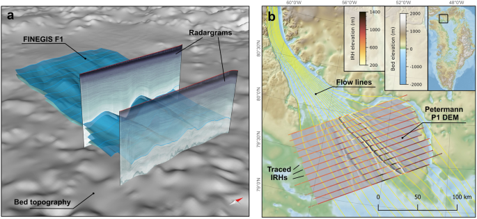
Example of the usage of different file formats. (a) A 3D canvas in Move where two of the FINEGIS GoCAD mesh objects have been imported. Furthermore, two RES sections (imported as a SEGY) and the bed topography (imported as a GeoTIFF) are shown. (b) The hillshaded Petermann Glacier P1 DEM is superimposed on Greenland’s bed topography47 in a QGIS 2D canvas. The color-coded vertical lines show the elevation of the traced isochrones (imported into QGIS from the xyz ASCII Line Set data). The yellow lines represent flow lines of the ice surface velocity85.

Nomenclature of file names
The file names for the different datasets are organized in the following systematic to specify the region, horizon age, geometry and file type: “[Region]_[Horizon]_[Version]_[age]_[subset]_[geometry].[filetype]”, e.g., Petermann_P1_V001_12_0_ka_mesh.dat for the P1 12.0 ka horizon mesh point cloud in the ASCII format. An overview and explanation for the field names are shown in Table 5.
File structure in PANGAEA
The various data formats of the 3D Horizons are archived in a Pangaea Publication Series. The entire data collection has an overarching DOI26. Each 3D horizon is stored as a data set in Publication Series: FINEGIS F1, FINEGIS F2, FINEGIS F3, NEGIS N1, Petermann P1, Petermann P2, Northern Central Greenland NG1, Northern Central Greenland NG2 (Table 6). Each data set contains several files of different data formats (ASCII, DEMs, GoCAD). Each dataset (e.g., FINEGIS F1) in turn, has its own DOI (Table 6). The download options can be accessed via the “View dataset as HTML” section. The entire dataset (i.e., all file formats) can be downloaded as a.zip or.tar archive, or the individual file formats can be downloaded separately.
Technical Validation
3D horizon geometry validation
For the 3D horizon construction, we preferred to use parallel RES profiles. For validating the interpolated geometries, we use those RES profiles that run obliquely to the main ones that were not used in the 3D horizon construction (Fig. 6). We have carried out this validation of the 3D geometry for all horizons published here.

Radargram that is oblique to the traced IRHs used for the 3D horizon construction and can be used to validate the resulting 3D horizon geometry independently.
Age validation
Because we converted our time-domain RES data into the elevation-domain with a constant dielectric permittivity of εice = 3.15, we also applied a firn correction of 10 m81 in all our horizons when linking the depth of the isochrone with the depth of the ice core. Furthermore, we considered various factors that may introduce a potential age error, such as (1) the range resolution of the RES system of ∼4.31 m58,71; (2) uncertainties in the determination of the surface reflection in the RES data (estimated uncertainty up to ∼5 m); (3) an error due to inaccuracies by the user who traces the isochrones in the radargrams (estimated to be two times the RES system range resolution; ∼10 m); (4) an error in the respective age scale (<1 m); (5) spatial variations in the density-depth function, either manifesting in a slightly different permittivity (e.g., from anisotropy) or a different firn correction (estimated to ∼5 m). Overall, we estimated the uncertainty in the age assignment to the horizons to be approximately ± 25 m relative to the depth of the respective ice-core time/depth scale. This means that the overall age error increases with depth (Table 3). Normalized to the absolute ages, the estimated age errors range between 2.5 and 7.5%. The errors given for the dating of the 3D horizons are thus relatively large, but we see potential in the future to minimize the errors for upcoming and existing 3D horizons by performing more precise determinations of the IRH ages, for example, with the use dielectric profiling measurements in combination with synthetic radar modelling78.
Usage Notes
Summary of data records
Petermann glacier
The data set from the onset region of Petermann Glacier19 consists of two 3D horizons (P1 and P2), which cover an area of approximately 156 × 95 km. Horizon P1 is ∼12.0 ± 0.9 ka old and approximately represents the transition from the Last Glacial period to the Holocene period and is located on average 1 km below the ice surface. The horizon is mainly characterized by open cylindrical folds with the fold axis oriented parallel to ice flow19 (Fig. 7a). The amplitudes of the folds reach up to 1 km with a wavelength of 10–15 km and are highest in the centre of the data set, corresponding to the region where ice flow converges towards the outlet glacier downstream. The deeper horizon P2 is ∼37.5 ± 2.1 ka old and shows increased folding intensity with slightly asymmetric and overturned folds. Nevertheless, the folds in P2 mimic those of the shallower P1 horizon (Fig. 7b). In contrast to P1, P2 shows gaps in regions where the 3D horizons could not be created due to uncertainties or poor visibility of the IRHs. Therefore, the datasets provided for horizon P2 are subdivided into P2A and P2B.

Individual 3D horizons published with this manuscript. Panels (a,b) represent the horizons from the onset of the Peterman Glacier, (c) the horizon at the NEGIS onset, centred at the EGRIP drill site, (d–f) the horizons upstream of the northern catchment of the 79NG (FINEGIS) and (g,h) the horizons covering northern central Greenland. The map in the background shows the bed topography47 overlain with a colour map of the surface ice flow velocity of Greenland85. It should be noted that the 3D horizons in are vertically exaggerated along the elevation axis by a factor of 15 for better visualization. A comparison between a vertically exaggerated 3D horizon and a non-exaggerated one representing the actual scale ratios is shown in Fig. 8 for the Petermann Glacier dataset.
Northeast greenland (FINEGIS)
The data set in northern Greenland upstream of the northern branch of the 79NG represents three 3D horizons (F1, F2 and F3), which are located close to the ice divide (Fig. 1). On average, the data span an area of 105 × 65 km. All three horizons show two cylindrical fold units that are visible in the lower third of the ice column21. The fold axes of these folds trend towards 100° (relative to true north) and show an increase in the degree of deformation (larger fold amplitudes) from the upper to the lower horizons (Fig. 7d–f). In contrast to the Peterman fold axes, the fold axes are oblique (∼25°) to the surface flow direction21. F1, F2 and F3 have ages of 45.5 ± 2.5, 52.2 ± 2.7, and 60.0 ± 4.0 ka, respectively. The two cylindrical folds are systematically overturned towards the north, whereby the degree of overturning increases downwards from F1 to F3. The deepest and oldest horizon, F3, is about 10% smaller in surface area than the two shallower horizons (Table 3).
NEGIS onset
The data set at the onset of NEGIS consists of one single 3D horizon (N1; 7.3 ± 0.2 ka), which covers an area of ∼250 × 90 km and is centred on the EastGRIP drill site (Fig. 1). The geometry of this 3D horizon shows a variety of complex folds with increasing fold density and intensity in the downstream direction. The shear margins are characterized by small wavelength (100–500 m) and small to moderate amplitude (∼100 m) folds that are oriented approximately parallel to the shear margins58. Each of these folds can be traced for tens of kilometres. In addition, long-wavelength (1–10 km) cylindrical folds are observed outside the ice stream. These folds form a fan-like pattern extending out from NEGIS (Fig. 7c). Close to the ice stream, the folds rotate towards parallelism with the shear margins while their wavelength decreases at the same time.
Northern central greenland
The data set in northern central Greenland covers the largest region in this data collection and consists of two horizons. The 3D horizons cover an area of approximately 690 × 55 km, reaching almost from the eastern to the western ice-sheet margins (Fig. 1). The shallower and thus younger horizon (NG1; 13.8 ± 1.0 ka old) is slightly larger in area than the deeper and older horizon (NG2; 37.5 ± 2.1 ka old). NG1 extends in the east into the NEGIS trunk and shows short-wavelength folds similar to those observed in the NEGIS shear margins (horizon N1; Fig. 7g). NG1 and NG2 reveal several upright cylindrical folds at each end, i.e., in the east and west of the covered area. The axes of the cylindrical folds in the west trend approximately west, whereas in the east, they trend towards the north. In the central-western area of NG1 and NG2, we find a large trough in the bed topography due to the paleofluvial mega-canyon65, which is imprinted in the 3D horizons that mimic this bed depression. In the centre of the covered area, near the main ice divide, we find upright cylindrical folds that trend to the north and northwest (Fig. 7g,h).
Potential applications of 3D horizons
The utilization of a 3D representation of IRHs in Greenland and Antarctica can contribute significantly to future studies and expand our understanding of the present-day and past behaviour of these environments. The features visible in the single sections are not necessarily linked directly to bed topography and surface ice flow velocity, data which is often used to plan the grid of a radar survey. The added value of a 3D horizon in comparison to the analysis of single IRHs is that it immediately reveals the geometry of structures independently of the grid layout. By examining the depth, continuity and geometry of these 3D horizons we can infer information on e.g., past and present ice flow patterns, basal conditions and properties and internal deformation processes19,21. Future studies can use this three-dimensional information to calibrate and refine ice-sheet models82,83 assess ice mass loss or gain and better predict the response of both ice-sheets to a warming climate. 3D horizons also provide a detailed view of the age structure within an ice sheet and provide, thus, valuable information on ice-sheet structure and dynamics. Furthermore, 3D horizons hold the potential to reveal information about past accumulation23,84. Altogether, this knowledge is crucial for understanding ice-sheet stability and their influence on ice-sheet dynamics .

Difference between a fifteen-times vertically exaggerated (a) and not exaggerated (b) view on the Petermann Glacier P1 12.0 ka horizon.
Code availability
The CReSIS toolbox used to process the MCoRDS RES data is available at https://gitlab.com/openpolarradar/opr, and the main documentation can be found at https://gitlab.com/openpolarradar/opr/-/wikis/home.
References
Khan, S. A. et al. Greenland ice sheet mass balance: a review. Rep Prog Phys 78, 046801, https://doi.org/10.1088/0034-4885/78/4/046801 (2015).
Hörhold, M. et al. Modern temperatures in central–north Greenland warmest in past millennium. Nature 613, 503–507, https://doi.org/10.1038/s41586-022-05517-z (2023).
Rietbroek, R., Brunnabend, S.-E., Kusche, J., Schröter, J. & Dahle, C. Revisiting the contemporary sea-level budget on global and regional scales. Proc National Acad Sci 113, 1504–1509, https://doi.org/10.1073/pnas.1519132113 (2016).
Holland, D. M., Thomas, R. H., Young, B., de, Ribergaard, M. H. & Lyberth, B. Acceleration of Jakobshavn Isbræ triggered by warm subsurface ocean waters. Nat Geosci 1, 659–664, https://doi.org/10.1038/ngeo316 (2008).
Jenkins, A. Convection-Driven Melting near the Grounding Lines of Ice Shelves and Tidewater Glaciers. J Phys Oceanogr 41, 2279–2294, https://doi.org/10.1175/jpo-d-11-03.1 (2011).
Choi, Y., Morlighem, M., Rignot, E. & Wood, M. Ice dynamics will remain a primary driver of Greenland ice sheet mass loss over the next century. Commun Earth Environ 2, 26, https://doi.org/10.1038/s43247-021-00092-z (2021).
Khan, S. A. et al. Extensive inland thinning and speed-up of Northeast Greenland Ice Stream. Nature 1–6, https://doi.org/10.1038/s41586-022-05301-z (2022).
MacGregor, J. A. et al. Radiostratigraphy and age structure of the Greenland Ice Sheet. J Geophys Res Earth Surf 120, 212–241, https://doi.org/10.1002/2014jf003215 (2015).
Gogineni, S. et al. Coherent radar ice thickness measurements over the Greenland ice sheet. J Geophys Res Atmospheres 106, 33761–33772, https://doi.org/10.1029/2001jd900183 (2001).
Schroeder, D. M. et al. Five decades of radioglaciology. Ann Glaciol 61, 1–13, https://doi.org/10.1017/aog.2020.11 (2020).
MacGregor, J. A. et al. The Scientific Legacy of NASA’s Operation IceBridge. Rev Geophys 59, https://doi.org/10.1029/2020rg000712 (2021).
Fujita, S. et al. Nature of radio echo layering in the Antarctic Ice Sheet detected by a two‐frequency experiment. J Geophys Res Solid Earth 104, 13013–13024, https://doi.org/10.1029/1999jb900034 (1999).
Millar, D. H. M. Radio-echo layering in polar ice sheets and past volcanic activity. Nature 292, 441–443, https://doi.org/10.1038/292441a0 (1981).
Robin, G. D. Q., Evans, S. & Bailey, J. T. Interpretation of radio echo sounding in polar ice sheets. Philosophical Transactions Royal Soc Lond Ser Math Phys Sci 265, 437–505, https://doi.org/10.1098/rsta.1969.0063 (1969).
Bodart, J. A. et al. Age-Depth Stratigraphy of Pine Island Glacier Inferred From Airborne Radar and Ice‐Core Chronology. J Geophys Res Earth Surf 126, https://doi.org/10.1029/2020jf005927 (2021).
Cavitte, M. G. P. et al. Deep radiostratigraphy of the East Antarctic plateau: connecting the Dome C and Vostok ice core sites. J Glaciol 62, 323–334, https://doi.org/10.1017/jog.2016.11 (2016).
Cavitte, M. G. P. et al. A detailed radiostratigraphic data set for the central East Antarctic Plateau spanning from the Holocene to the mid-Pleistocene. Earth Syst Sci Data 13, 4759–4777, https://doi.org/10.5194/essd-13-4759-2021 (2021).
Winter, A., Steinhage, D., Creyts, T. T., Kleiner, T. & Eisen, O. Age stratigraphy in the East Antarctic Ice Sheet inferred from radio-echo sounding horizons. Earth Syst Sci Data 11, 1069–1081, https://doi.org/10.5194/essd-11-1069-2019 (2019).
Bons, P. D. et al. Converging flow and anisotropy cause large-scale folding in Greenland’s ice sheet. Nat Commun 7, 11427, https://doi.org/10.1038/ncomms11427 (2016).
Franke, S. Decoding ice flow history from englacial radar stratigraphy. Nat Rev Earth Environ 1–1, https://doi.org/10.1038/s43017-023-00390-4 (2023).
Franke, S. et al. Holocene ice-stream shutdown and drainage basin reconfiguration in northeast Greenland. Nat Geosci 15, 995–1001, https://doi.org/10.1038/s41561-022-01082-2 (2022).
Bingham, R. G. et al. Ice‐flow structure and ice dynamic changes in the Weddell Sea sector of West Antarctica from radarimaged internal layering. J Geophys Res Earth Surf 120, 655–670, https://doi.org/10.1002/2014jf003291 (2015).
Bodart, J. A. et al. High mid-Holocene accumulation rates over West Antarctica inferred from a pervasive ice-penetrating radar reflector. Cryosphere 17, 1497–1512, https://doi.org/10.5194/tc-17-1497-2023 (2023).
Holschuh, N., Christianson, K., Conway, H., Jacobel, R. W. & Welch, B. C. Persistent tracers of historic ice flow in glacial stratigraphy near Kamb Ice Stream, West Antarctica. Cryosphere 12, 2821–2829, https://doi.org/10.5194/tc-12-2821-2018 (2018).
Siegert, M. J. et al. Ice Flow Direction Change in Interior West Antarctica. Science 305, 1948–1951, https://doi.org/10.1126/science.1101072 (2004).
Franke, S. et al. Three-dimensional anatomy of folded radar stratigraphy in polar ice sheets [data set]. PANGAEA https://doi.org/10.1594/pangaea.954991 (2023).
Münchow, A., Padman, L. & Fricker, H. A. Interannual changes of the floating ice shelf of Petermann Gletscher, North Greenland, from 2000 to 2012. J Glaciol 60, 489–499, https://doi.org/10.3189/2014jog13j135 (2014).
Rignot, E. & Steffen, K. Channelized bottom melting and stability of floating ice shelves. Geophys Res Lett 35, https://doi.org/10.1029/2007gl031765 (2008).
Nick, F. M. et al. The response of Petermann Glacier, Greenland, to large calving events, and its future stability in the context of atmospheric and oceanic warming. J Glaciol 58, 229–239, https://doi.org/10.3189/2012jog11j242 (2012).
Rückamp, M., Neckel, N., Berger, S., Humbert, A. & Helm, V. Calving Induced Speedup of Petermann Glacier. J Geophys Res Earth Surf 124, 216–228, https://doi.org/10.1029/2018jf004775 (2019).
Åkesson, H., Morlighem, M., O’Regan, M. & Jakobsson, M. Future Projections of Petermann Glacier Under Ocean Warming Depend Strongly on Friction Law. J Geophys Res Earth Surf 126, https://doi.org/10.1029/2020jf005921 (2021).
Åkesson, H., Morlighem, M., Nilsson, J., Stranne, C. & Jakobsson, M. Petermann ice shelf may not recover after a future breakup. Nat Commun 13, 2519, https://doi.org/10.1038/s41467-022-29529-5 (2022).
Hill, E. A., Gudmundsson, G. H., Carr, J. R., Stokes, C. R. & King, H. M. Twenty-first century response of Petermann Glacier, northwest Greenland to ice shelf loss. J Glaciol 67, 147–157, https://doi.org/10.1017/jog.2020.97 (2021).
Morlighem, M., Rignot, E., Mouginot, J., Seroussi, H. & Larour, E. Deeply incised submarine glacial valleys beneath the Greenland ice sheet. Nat Geosci 7, 418–422, https://doi.org/10.1038/ngeo2167 (2014).
Chu, W., Schroeder, D. M., Seroussi, H., Creyts, T. T. & Bell, R. E. Complex Basal Thermal Transition Near the Onset of Petermann Glacier, Greenland. J Geophys Res Earth Surf 123, 985–995, https://doi.org/10.1029/2017jf004561 (2018).
Bell, R. E. et al. Deformation, warming and softening of Greenland’s ice by refreezing meltwater. Nat Geosci 7, 497–502, https://doi.org/10.1038/ngeo2179 (2014).
Panton, C. & Karlsson, N. B. Automated mapping of near bed radio-echo layer disruptions in the Greenland Ice Sheet. Earth Planet Sc Lett 432, 323–331, https://doi.org/10.1016/j.epsl.2015.10.024 (2015).
Vieli, G. J.-M. C. L., Martín, C., Hindmarsh, R. C. A. & Lüthi, M. P. Basal freeze-on generates complex ice-sheet stratigraphy. Nat Commun 9, 4669, https://doi.org/10.1038/s41467-018-07083-3 (2018).
Wolovick, M. J., Creyts, T. T., Buck, W. R. & Bell, R. E. Traveling slippery patches produce thickness‐scale folds in ice sheets. Geophys Res Lett 41, 8895–8901, https://doi.org/10.1002/2014gl062248 (2014).
Dow, C. F., Karlsson, N. B. & Werder, M. A. Limited Impact of Subglacial Supercooling Freeze‐on for Greenland Ice Sheet Stratigraphy. Geophys Res Lett 45, 1481–1489, https://doi.org/10.1002/2017gl076251 (2018).
Aschwanden, A., Fahnestock, M. A. & Truffer, M. Complex Greenland outlet glacier flow captured. Nat Commun 7, 10524, https://doi.org/10.1038/ncomms10524 (2016).
Krieger, L., Floricioiu, D. & Neckel, N. Drainage basin delineation for outlet glaciers of Northeast Greenland based on Sentinel-1 ice velocities and TanDEM-X elevations. Remote Sens Environ 237, 111483, https://doi.org/10.1016/j.rse.2019.111483 (2020).
Mouginot, J. et al. Forty-six years of Greenland Ice Sheet mass balance from 1972 to 2018. Proc National Acad Sci 116, 9239–9244, https://doi.org/10.1073/pnas.1904242116 (2019).
Khan, S. A. et al. Sustained mass loss of the northeast Greenland ice sheet triggered by regional warming. Nat Clim Change 4, 292–299, https://doi.org/10.1038/nclimate2161 (2014).
Choi, Y., Morlighem, M., Rignot, E., Mouginot, J. & Wood, M. Modeling the Response of Nioghalvfjerdsfjorden and Zachariae Isstrøm Glaciers, Greenland, to Ocean Forcing Over the Next Century. Geophys Res Lett 44, 11,071–11,079, https://doi.org/10.1002/2017gl075174 (2017).
Grinsted, A. et al. Accelerating ice flow at the onset of the Northeast Greenland Ice Stream. Nat Commun 13, 5589, https://doi.org/10.1038/s41467-022-32999-2 (2022).
Morlighem, M. et al. BedMachine v3: Complete Bed Topography and Ocean Bathymetry Mapping of Greenland From Multibeam Echo Sounding Combined With Mass Conservation. Geophys Res Lett 44, 11,051–11,061, https://doi.org/10.1002/2017gl074954 (2017).
Franke, S. et al. Bed topography and subglacial landforms in the onset region of the Northeast Greenland Ice Stream. Ann Glaciol 61, 143–153, https://doi.org/10.1017/aog.2020.12 (2020).
Fahnestock, M., Abdalati, W., Joughin, I., Brozena, J. & Gogineni, P. High Geothermal Heat Flow, Basal Melt, and the Origin of Rapid Ice Flow in Central Greenland. Science 294, 2338–2342, https://doi.org/10.1126/science.1065370 (2001).
Vallelonga, P. et al. Initial results from geophysical surveys and shallow coring of the Northeast Greenland Ice Stream (NEGIS). Cryosphere 8, 1275–1287, https://doi.org/10.5194/tc-8-1275-2014 (2014).
Christianson, K. et al. Dilatant till facilitates ice-stream flow in northeast Greenland. Earth Planet Sc Lett 401, 57–69, https://doi.org/10.1016/j.epsl.2014.05.060 (2014).
Keisling, B. A. et al. Basal conditions and ice dynamics inferred from radar-derived internal stratigraphy of the northeast Greenland ice stream. Ann Glaciol 55, 127–137, https://doi.org/10.3189/2014aog67a090 (2014).
Smith-Johnsen, S., Fleurian, B., de, Schlegel, N., Seroussi, H. & Nisancioglu, K. Exceptionally high heat flux needed to sustain the Northeast Greenland Ice Stream. Cryosphere 14, 841–854, https://doi.org/10.5194/tc-14-841-2020 (2020).
Bons, P. D. et al. Comment on “Exceptionally high heat flux needed to sustain the Northeast Greenland Ice Stream” by Smith-Johnsen et al. (2020). Cryosphere 15, 2251–2254, https://doi.org/10.5194/tc-15-2251-2021 (2021).
Westhoff, J. et al. A stratigraphy-based method for reconstructing ice core orientation. Ann Glaciol 62, 191–202, https://doi.org/10.1017/aog.2020.76 (2021).
Gerber, T. A. et al. Upstream flow effects revealed in the EastGRIP ice core using Monte Carlo inversion of a two-dimensional ice-flow model. Cryosphere 15, 3655–3679, https://doi.org/10.5194/tc-15-3655-2021 (2021).
Hvidberg, C. S. et al. Surface velocity of the Northeast Greenland Ice Stream (NEGIS): assessment of interior velocities derived from satellite data by GPS. Cryosphere 14, 3487–3502, https://doi.org/10.5194/tc-14-3487-2020 (2020).
Franke, S. et al. Airborne ultra-wideband radar sounding over the shear margins and along flow lines at the onset region of the Northeast Greenland Ice Stream. Earth Syst Sci Data 14, 763–779, https://doi.org/10.5194/essd-14-763-2022 (2022).
Franke, S. et al. Complex Basal Conditions and Their Influence on Ice Flow at the Onset of the Northeast Greenland Ice Stream. J Geophys Res Earth Surf 126, https://doi.org/10.1029/2020jf005689 (2021).
Zeising, O. & Humbert, A. Indication of high basal melting at the EastGRIP drill site on the Northeast Greenland Ice Stream. Cryosphere 15, 3119–3128, https://doi.org/10.5194/tc-15-3119-2021 (2021).
Zeising, O. et al. Improved estimation of the bulk ice crystal fabric asymmetry from polarimetric phase co-registration. Cryosphere 17, 1097–1105, https://doi.org/10.5194/tc-17-1097-2023 (2023).
Lilien, D. A., Rathmann, N. M., Hvidberg, C. S. & Dahl‐Jensen, D. Modeling Ice‐Crystal Fabric as a Proxy for Ice‐Stream Stability. J Geophys Res Earth Surf 126, https://doi.org/10.1029/2021jf006306 (2021).
Oraschewski, F. M. & Grinsted, A. Modeling enhanced firn densification due to strain softening. Cryosphere 16, 2683–2700, https://doi.org/10.5194/tc-16-2683-2022 (2022).
Gerber, T. A. et al. Crystal orientation fabric anisotropy causes directional hardening of the Northeast Greenland Ice Stream. Nat Commun 14, 2653, https://doi.org/10.1038/s41467-023-38139-8 (2023).
Bamber, J. L., Siegert, M. J., Griggs, J. A., Marshall, S. J. & Spada, G. Paleofluvial Mega-Canyon Beneath the Central Greenland Ice Sheet. Science 341, 997–999, https://doi.org/10.1126/science.1239794 (2013).
Rodriguez-Morales, F. et al. Advanced Multifrequency Radar Instrumentation for. Polar Research. Ieee T Geosci Remote 52, 2824–2842, https://doi.org/10.1109/tgrs.2013.2266415 (2013).
Hale, R. et al. Multi-Channel Ultra-Wideband Radar Sounder and Imager. 2016 Ieee Int Geoscience Remote Sens Symposium Igarss 2112–2115, https://doi.org/10.1109/igarss.2016.7729545 (2016).
Alfred-Wegener-Institut Helmholtz-Zentrum für Polar- und Meeresforschung. Polar aircraft Polar5 and Polar6 operated by the Alfred Wegener Institute. J Large-scale Res Facil Jlsrf 2, 87, https://doi.org/10.17815/jlsrf-2-153 (2016).
CReSIS Toolbox (Version 3.0.1). Zenodo https://doi.org/10.5281/zenodo.5683959 (2021).
CReSIS Open Polar Server. https://ops.cresis.ku.edu/.
CReSIS RDS Documentation. https://data.cresis.ku.edu/data/rds/rds_readme.pdf.
Bohleber, P., Wagner, N. & Eisen, O. Permittivity of ice at radio frequencies: Part I. Coaxial transmission line cell. Cold Reg Sci Technol 82, 56–67, https://doi.org/10.1016/j.coldregions.2012.05.011 (2012).
Howat, I. M., Negrete, A. & Smith, B. E. The Greenland Ice Mapping Project (GIMP) land classification and surface elevation data sets. Cryosphere 8, 1509–1518, https://doi.org/10.5194/tc-8-1509-2014 (2014).
Beyreuther, M. et al. ObsPy: A Python Toolbox for Seismology. Seismol Res Lett 81, 530–533, https://doi.org/10.1785/gssrl.81.3.530 (2010).
CReSIS Data Products. https://data.cresis.ku.edu/.
Mojtabavi, S. et al. A first chronology for the East Greenland Ice-core Project (EGRIP) over the Holocene and last glacial termination. Clim Past 16, 2359–2380, https://doi.org/10.5194/cp-16-2359-2020 (2020).
Rasmussen, S. O. et al. A first chronology for the North Greenland Eemian Ice Drilling (NEEM) ice core. Clim Past 9, 2713–2730, https://doi.org/10.5194/cp-9-2713-2013 (2013).
Eisen, O., Wilhelms, F., Steinhage, D. & Schwander, J. Improved method to determine radio-echo sounding reflector depths from ice-core profiles of permittivity and conductivity. J Glaciol 52, 299–310, https://doi.org/10.3189/172756506781828674 (2006).
Conrad, O. et al. System for Automated Geoscientific Analyses (SAGA) v. 2.1.4. Geosci Model Dev 8, 1991–2007, https://doi.org/10.5194/gmd-8-1991-2015 (2015).
Haber, J., Zeilfelder, F., Davydov, O. & Seidel, H.-P. Smooth Approximation and Rendering of Large Scattered Data Sets. Proc Vis 2001 Vis’01 341–205, https://doi.org/10.1109/visual.2001.964530 (2001).
Hempel, L., Thyssen, F., Gundestrup, N., Clausen, H. B. & Miller, H. A comparison of radio-echo sounding data and electrical conductivity of the GRIP ice core. J Glaciol 46, 369–374, https://doi.org/10.3189/172756500781833070 (2000).
Sutter, J., Fischer, H. & Eisen, O. Investigating the internal structure of the Antarctic ice sheet: the utility of isochrones for spatiotemporal ice-sheet model calibration. Cryosphere 15, 3839–3860, https://doi.org/10.5194/tc-15-3839-2021 (2021).
Višnjević, V. et al. Predicting the steady-state isochronal stratigraphy of ice shelves using observations and modeling. Cryosphere 16, 4763–4777, https://doi.org/10.5194/tc-16-4763-2022 (2022).
Karlsson, N. B., Dahl-Jensen, D., Gogineni, S. P. & Paden, J. D. Tracing the depth of the Holocene ice in North Greenland from radio-echo sounding data. Ann Glaciol 54, 44–50, https://doi.org/10.3189/2013aog64a057 (2013).
Joughin, I., Smith, B. E. & Howat, I. M. A complete map of Greenland ice velocity derived from satellite data collected over 20 years. J Glaciol 64, 1–11, https://doi.org/10.1017/jog.2017.73 (2018).
Acknowledgements
We thank the crew of the research aircraft Polar6 and system engineers M. Gehrmann and L. Kandora. We acknowledge the use of the CReSIS toolbox and using RES data from CReSIS generated with support from the University of Kansas, NASA Operation IceBridge grant NNX16AH54G, NSF grants ACI-1443054, OPP-1739003 and IIS-1838230, Lilly Endowment Incorporated and Indiana METACyt Initiative. Furthermore, we acknowledge the Academic Software Initiative for using Move for the generation of parts of the data published here. We thank the EGRIP project for logistical support during the EGRIP-NOR-2018 RES campaign. EGRIP is directed and organized by the Centre for Ice and Climate at the Niels Bohr Institute, University of Copenhagen. It is supported by funding agencies and institutions in Denmark (A. P. Møller Foundation, University of Copenhagen), the United States (US National Science Foundation, Office of Polar Programs), Germany (Alfred Wegener Institute, Helmholtz Centre for Polar and Marine Research), Japan (National Institute of Polar Research and Arctic Challenge for Sustainability), Norway (University of Bergen and Trond Mohn Foundation), Switzerland (Swiss National Science Foundation), France (French Polar Institute Paul-Emile Victor, Institute for Geosciences and Environmental Research), Canada (University of Manitoba) and China (Chinese Academy of Sciences and Beijing Normal University). Steven Franke was funded by the AWI Strategy fund and the Walter Benjamin Programme of the Deutsche Forschungsgemeinschaft (DFG, German Research Foundation) – project number: 506043073. Daniela Jansen was funded by the AWI Strategy Fund and the Helmholtz Young Investigator Group HGF YIG VH-NG-802. Catherine C. Bauer was funded by the DFG (German Research Foundation), Grant number BA643/1-1.
Funding
Open Access funding enabled and organized by Projekt DEAL.
Author information
Authors and Affiliations
Contributions
S.F. wrote the manuscript. The 3D horizons were constructed by S.F., D.J., K.S., F.M., C.B. and P.D.B. Radio-echo sounding data were acquired by D.J., V.H., J.P. and T.B. and radio-echo sounding data processing was performed by S.F., D.J., V.H., J.P., T.B., N.D. and D.S. All authors commented and reviewed the manuscript.
Corresponding authors
Ethics declarations
Competing interests
The authors declare no competing interests.
Additional information
Publisher’s note Springer Nature remains neutral with regard to jurisdictional claims in published maps and institutional affiliations.
Rights and permissions
Open Access This article is licensed under a Creative Commons Attribution 4.0 International License, which permits use, sharing, adaptation, distribution and reproduction in any medium or format, as long as you give appropriate credit to the original author(s) and the source, provide a link to the Creative Commons license, and indicate if changes were made. The images or other third party material in this article are included in the article’s Creative Commons license, unless indicated otherwise in a credit line to the material. If material is not included in the article’s Creative Commons license and your intended use is not permitted by statutory regulation or exceeds the permitted use, you will need to obtain permission directly from the copyright holder. To view a copy of this license, visit http://creativecommons.org/licenses/by/4.0/.
About this article

Cite this article
Franke, S., Bons, P.D., Streng, K. et al. Three-dimensional topology dataset of folded radar stratigraphy in northern Greenland. Sci Data 10, 525 (2023). https://doi.org/10.1038/s41597-023-02339-0
Received:
Accepted:
Published:
DOI: https://doi.org/10.1038/s41597-023-02339-0
