
Abstract
Accurately characterizing clouds and their shadows is a long-standing problem in the Earth Observation community. Recent works showcase the necessity to improve cloud detection methods for imagery acquired by the Sentinel-2 satellites. However, the lack of consensus and transparency in existing reference datasets hampers the benchmarking of current cloud detection methods. Exploiting the analysis-ready data offered by the Copernicus program, we created CloudSEN12, a new multi-temporal global dataset to foster research in cloud and cloud shadow detection. CloudSEN12 has 49,400 image patches, including (1) Sentinel-2 level-1C and level-2A multi-spectral data, (2) Sentinel-1 synthetic aperture radar data, (3) auxiliary remote sensing products, (4) different hand-crafted annotations to label the presence of thick and thin clouds and cloud shadows, and (5) the results from eight state-of-the-art cloud detection algorithms. At present, CloudSEN12 exceeds all previous efforts in terms of annotation richness, scene variability, geographic distribution, metadata complexity, quality control, and number of samples.
Measurement(s) | clouds extension |
Technology Type(s) | machine learning with photo-interpretation. |
Factor Type(s) | Copernicus Sentinel-2 images |
Sample Characteristic - Environment | geosphere |
Sample Characteristic - Location | all the world |
Background & Summary
We are in the midst of an exciting new era of Earth observation (EO), wherein Analysis Ready Data (ARD)1,2,3 products derived from big optical satellite imagery catalogs permit direct analyses without laborious pre-processing. Unfortunately, many of these products are contaminated by clouds4 and their corresponding shadows, altering the surface reflectance values and hampering their operational exploitation at large scales. For most of the applications exploiting ARD, cloud and cloud-shadow pixels need to be removed prior to further analyses, i.e. masked out, to avoid distortions in the results.
Improving the accuracy of existing cloud detection (CD) algorithms used in current ARD products is a pressing need for the EO community regarding optical sensors such as Sentinel-2. Ideally, CD algorithms would classify pixels into clear, cloud shadow, thin cloud, and thick cloud. Splitting clouds into two subclasses allows downstream applications to design different strategies to treat cloud contamination. On the one hand, thick clouds entirely block the surface’s view, reflecting most of the light coming from the sun and generating gaps impossible to retrieve using optical sensors data5. On the other hand, thin clouds do not reflect all the sunlight allowing to observe a distorted view of the surface6,7. For some applications, such as object detection or disaster response8, images contaminated with thin clouds are still helpful. Therefore, distinguishing between thick and thin clouds is also a critical first step toward optical data exploitation. Nevertheless, it is worth noting that there is no overall consensus on quantitative approaches delimiting when one class begins and the other ends; thus, it is so far inherently subjective to the image interpreter9,10.
Methodologies for CD can be classified into two main categories: knowledge-driven (KD) and data-driven (DD). KD category emphasizes the logical sense connected with physical foundations. For instance, the Function of mask (Fmask)11 and Sen2Cor12 use a set of physical rules formulated on spectral and contextual features to distinguish clouds against water or land. Overall, KD algorithms achieve accurate results, and good generalization13,14,15. However, it is well-known that they have problems associated with thin cloud omission and non-cloud object commission, frequently at cloud edges and under surfaces with a smooth texture or high reflectance16,17.
In recent years, supervised data-driven strategies, trained in large manually annotated datasets, have grown notoriety in remote sensing thanks to the success of classical machine learning (ML) and deep learning (DL) techniques18. Among multiple noteworthy ML precedents19,20,21 in cloud detection, Sentinel Hub’s s2cloudless22 is the most extensively used due to its low computational requirements and lightweight design. Nonetheless, when evaluated in certain particular regions, such as tropical forests, s2cloudless falls short of state-of-the-art KD cloud detectors13,23,24. Meanwhile, DL has proven to be more effective on CD compared to more classical ML25,26, although it is subjected to the exigency of pixel-level annotation.
The recent progress in DL-based cloud semantic segmentation in Sentinel-2 can be attributed to the proliferation of public CD datasets such as SPARCS27, S2-Hollstein28, Biome 810, 38-cloud29, CESBIO30, 95-Cloud31, and CloudCatalogue32. Nonetheless, these datasets have some well-known shortcomings, including the absence of a temporal component, a lack of thin clouds or cloud shadows labels, a high degree of imbalance between cloud and non-cloud classes, and a relatively small size joined with geographical bias (see Table 1 for the current characteristics/limitations of each of those datasets). Furthermore, their quality control process is not always properly described and their development remains somehow unclear. Additionally, there is a lack of consensus on manual annotation protocols and cloud semantic classes definition, which makes inter-dataset comparison problematic, particularly under pixels where class transitions occur. These flaws hinder the natural transition to global DL cloud classifiers and the application of new-fashioned geographically-aware algorithms13.
Inspired by the CityScapes dataset33, we created and released CloudSEN12, a large and globally distributed dataset (Fig. 1) for cloud semantic understanding based mainly on Sentinel 2 imagery. CloudSEN12 surpasses all previous efforts in size and variability (see Table 1), offering 49,250 image patches (IPs) with different annotation types: (i) 10,000 IPs with high-quality pixel-level annotation, (ii) 10,000 IPs with scribble annotation, and (iii) 29,250 unlabeled IPs. The labeling phase was conducted by 14 domain experts using a supervised active learning system. We designed a rigorous four-step quality control protocol based on Zhu et al.34 to guarantee high quality in the manual annotation phase. Furthermore, CloudSEN12 ensures that for the same geographical location, users can obtain multiple IPs with different cloud coverage: cloud-free (0%), almost-clear (0–25%), low-cloudy (25–45%), mid-cloudy (45–65%), and cloudy (>65%), which ensures scene variability in the temporal domain. Finally, to support multi-modal cloud removal35 and data fusion36 approaches, each CloudSEN12 IP includes data from various remote sensing sources that have already shown their usefulness in cloud and cloud shadow masking, such as Sentinel-1 and elevation data. See Table 2 for a full list of assets available for each image patch.

CloudSEN12 spatial coverage, purple-to-yellow color gradient represents the amount of manually annotated pixels per hexagon. The annotated pixels were collocated in an equal-area hexagonal discrete grid with a facet size of 140 km.
Methods
This study collects and combines several public data sources that may potentially help us to annotate cloud and cloud shadows better. Based on this information, semantic classes (Table 3) are created using an active system that blends human photo interpretation and machine learning. Finally, a strict quality control protocol is carried out to ensure the highest quality on the manual labels and to establish human-level performance. Figure 2 depicts the whole workflow followed to create the dataset. Figure 2a depicts all available data in each CloudSEN12 IP (see Method:Data preparation section). Figure 2b illustrates the manual IP selection strategy realized in each ROI (see Method:Image patches selection section). Finally, Fig. 2c highlights the human annotation strategy and cloud detection models offered in each IP (see Method:Annotation strategy and Method:Available cloud detection models sections).

A high-level summary of our workflow to generate IPs. (a) Satellite imagery datasets that comprises CloudSEN12 assets. (b) IP selection by the CDE group. (c) Generation of manual and automatic cloud masking. KappasMask and CD-FCNN have two distinct configurations.
Data preparation
CloudSEN12 comprises different free and open datasets provided by several public institutions and made accessible by the Google Earth Engine (GEE) platform37. These include Sentinel-2A/B (SEN2), Sentinel-1A/B (SEN1), Multi-Error-Removed Improved-Terrain (MERIT) DEM38, Global Surface Water39 (GSW), and Global Land Cover maps40 at 10 and 100 meters. The SEN1 and SEN2 multi-spectral image data correspond to the 2018–2020 period. We included all the bands from both SEN2 top-of-atmosphere (TOA) reflectance (Level-1C) and SEN2 surface reflectance (SR) values (Level-2A) derived from the Sen2Cor processor, which can be useful to analyze the impact of CD algorithms on atmospherically corrected derived products. See S2L1C and S2L2A in Table 2 for band description. On the other hand, SEN1 acquires data with a revisit cycle between 6–12 days according to four standard operational modes: Stripmap (SM), Extra Wide Swath (EW), Wave (WV), and Interferometric Wide Swath (IW). In CloudSEN12, we collect IW data with two polarization channels (VV and VH) from the high-resolution Level-1 Ground Range Detected (GRD) product. Furthermore, we saved the approximate angle between the incident SAR beam and the reference ellipsoid (see S1 in Table 2). Lastly, our dataset also includes previously proposed features for cloud semantic segmentation such as (1) Cloud Displacement Index41, (2) the azimuth (0–360°) calculated using the solar azimuth and zenith angles42 from SEN2 metadata, (3) elevation from MERIT dataset, (4) land cover maps from the Copernicus Global Land Service (CGLS) version 3, and the ESA WorldCover 10 m v100, and (5) water occurrence from the GSW dataset (see extra/ in Table 2). All the previous features constitute the raw CloudSEN12 imagery dataset (Fig. 2a). All the image scenes in raw CloudSEN12 were resampled to 10 meters using local SEN2 UTM coordinates.
Image patches selection
We sampled 20,000 random regions of interest (ROIs) dispersed globally in order to retrieve raw CloudSEN12 data. Each ROI has a dimension of 5,090 × 5,090 meters. Besides, we carefully added 5,000 manually selected ROIs to guarantee high scene diversity on complicated surfaces such as snow and built-up areas. Afterwards, an ROI is retained in the dataset if all three of the following requirements are met: (1) SEN2 Level-1C IP does not include saturated or no-data pixel values, (2) the time difference between SEN1 and SEN2 acquisitions is not higher than 2.5 days, and (3) there are more than 15 SEN2 Level-1C image scenes for the given ROI after applying (2). The total number of ROIs decreased from 25,000 to 12,121 as a result of this filtering. Despite this reduction, CloudSEN12 still manages to reach a full global representation. However, a high number of ROIs does not necessarily imply a consistent distribution among cloud types and coverage. Unfortunately, image selection based on automatic cloud masking or cloud cover metadata tends to produce misleading results, especially under high-altitude areas43, intricate backgrounds44, and mixed cloud types scenes. Hence, to guarantee unbiased distribution between clear, cloud and cloud shadow pixels, 14 cloud detection experts manually selected the IPs (hereafter referred to as CDE group, Fig. 2b). For each ROI, we pick five IPs with different cloud coverage: cloud-free (0%), almost-clear (0–25%), low-cloudy (25–65%), mid-cloudy (45–65%), and cloudy image (>65%). Atypical clouds such as contrails, ice clouds, and haze/fog had a higher priority than common clouds (i.e., cumulus and stratus). After eliminating ROIs that did not count with at least one IP for each cloud coverage class, the total number of ROIs was reduced from 12,121 to 9,880, resulting in the final CloudSEN12 spatial coverage (Fig. 1).
Annotation strategy
New trends in computer vision show that reformulating the standard supervised learning scheme can alleviate the huge demands of hand-crafted labeled data. For instance, semi-supervised learning can produce more detailed and uniform predictions45, while weakly-supervised learning suggests a more cost-effective option to pixel-wise annotation in semantic segmentation. Users might utilize scribble labels to train a model for coarse-to-fine enrichment46. Aware of these manual labeling requirements, CloudSEN12 includes three types of labeling data: high-quality, scribble, and no-annotation. Consequently, each ROI is randomly assigned to a distinct annotation category (Fig. 2c) and labelled by the CDE group:
-
2,000 ROIs with pixel level annotation, where the average annotation time is 150 minutes (high-quality subset, Fig. 3a).
Fig. 3 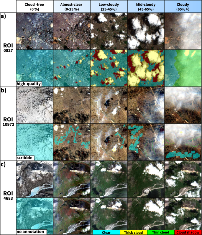
The three primary types of hand-crafted labeling data available in CloudSEN12. The first row in high-quality (a), scribble (b), and no annotation (c) subgroups shows a SEN2 level 1 C RGB band combination.
-
2,000 ROIs with scribble level annotation, where the annotation time is 16 minutes (scribble subset, Fig. 3b).
-
5,880 ROIs with annotation only in the cloud-free (0%) image (no annotation subset, Fig. 3c).

Human calibration phase
Human photo interpretation is not a faultless procedure. It might easily be skewed by an individual’s basis, overconfidence, tiredness, or ostrich-effect47 proclivity. Hence, to lessen this effect, the CDE group refined their criteria using a “calibration” dataset composed of 35 manually selected challenging IPs. In this stage, all the labelers can consult each other. As a result, they reached an agreement about the SEN2 band compositions to be used and how to deal with complicated scenarios such as cloud boundaries, thin cloud shadows, and high-reflectance background. A labeler is considered fully trained if its overall accuracy in the calibration dataset surpasses 90%. Then, a “validation” dataset formed of ten IPs is used to assess individual performance; labelers are not permitted to confer with one another during this step. If the labeler’s overall accuracy drops below 90%, it will return to the calibration phase (Fig. 4).

Human calibration workflow diagram. The overall accuracy (OA) is calculated by comparing individual labeler results against expert group results.
Labeling phase
The Intelligence foR Image Segmentation (IRIS) active learning software48 was used in the manual labeling annotation process (Supplementary Fig. S1). IRIS allowed CDE members to train a model (learner) with a small set of labeled samples that is iteratively reinforced by acquiring new samples provided by a labeler (oracle). As a result, it dramatically decreases the time spent creating hand-crafted labels but maintains the labeler’s capacity to make final manual revisions if necessary. For high-quality labeling generation (Fig. 5a), IRIS starts training a gradient boosting decision tree (GBDT)49 with s2cloudless cloud probability values greater than 0.7 as thick cloud and less than 0.3 as clear. GBDT algorithm starts generating weak decision trees by dividing training data and gradually moving in the direction of lowering the loss function, then all the weak decision trees are combined into a single strong learner to generate a final prediction. IRIS use the LightGBM Python package. Readers are referred to Ke et al.50 for a detailed algorithm description. After obtaining GBDT predictions, the CDE group makes adjustments to the prior results and, if necessary, adds other cloud semantic classes such as cloud shadow and thin cloud. Using this new sample set, the GBDT model is re-trained. The two previous steps are repeated several times until the pixel-wise annotation passes the labeler’s visual inspection filter. The final high-quality annotation results are then obtained by applying extra manual fine-tuning. Since there are no quantitative criteria to distinguish between boundaries in semantic classes, the labelers always attempt to maximize the sensitivity score under ambiguous edges.

(a) High-quality labeling phase diagram. The model is set up using s2cloudless priors (blue). Annotations made by labelers with and without ML assistance are saved (green). (b) Scribble labeling phase diagram. The labelers starts by adding samples at the centroids (blue), and then into the borders; if the results pass a simple visual inspection, the annotation is send to inspection (see Method:Quality control phase section).
On the other hand, for scribble labeling (Fig. 5b), the CDE group also used IRIS but without ML assistance. First, labelers spend one-minute adding annotations around centroids of the semantic classes. Usually, pixels adjacent to the centroids are more straightforward to classify automatically. Then, to produce balanced annotations, the CDE group added more samples at cloud and cloud shadow edges for three more minutes.
Quality control phase
Despite the human calibration phase, errors are still common in hand-operated labels. Therefore, statistic and visual inspections were implemented before admitting a manual annotation in CloudSEN12 (Fig. 6). First, an automatic check is set only for high-quality labels. It proposes that the GBDT accuracy during training must be higher than 0.95. This simple threshold pushes the CDE group to set more samples and care more about labeling correctness. Later, two sequential visual inspection rounds are carried out for scribble and high-quality labels. The evaluators are two other CDE members than the one who labeled the IP. If a mistake is found, it is notified using GitHub Discussions (https://github.com/cloudsen12/models/discussions). Finally, we discern the most challenging IPs (difficulty level greater than 4, see Table 4) and consult all CDE members to reaffirm or change a semantic class. The deliberations were supported by using cloudApp (https://csaybar.users.earthengine.app/view/cloudapp), which is a GEE web application that displays SEN2 image time series from any location on the earth (Supplementary Fig. S2).

Flowchart overview of the entire QC process.
Comparing the manual annotation before and after quality control can provide insight into the correctness of annotations made by humans. Based on this, CloudSEN12 set, for the first time, the human-level performance at 95.7% confidence when considering all semantic cloud classes (described in Table 3) and 98.3% if thin clouds are discarded. The clear and thick cloud classes presented the largest PA agreement with 99.1% and 96.6%, respectively (Fig. 7). The variance concerning the thick cloud class (3.4%) was produced by efforts to limit the formation of false positives around cloud borders in the first round of quality control. In contrast, thin cloud and cloud shadow classes present the largest disparities, with a PA of 78 and 91.8%, respectively. Despite using IRIS and CloudApp, which permits labelers to contrast both spectral and temporal SEN2 data, the detection of semi-transparent clouds remained unclear (21%). This was especially noticeable when all CDE members discussed the most complicated IPs (Fig. 6); thin clouds were always the source of the most contention. Considering the assimilation of atmospheric reanalysis data and radiative transfer model outputs could help to reduce the cirrus detection uncertainty9,51. Nonetheless, our manual labeling approach did not consider this additional data. Finally, cloud shadow disagreement is explained by a reinterpretation of the semantic classes after the first quality control round. At first, we assumed that only thick clouds could project shadows. However, this was ruled out as many thin low-altitude clouds project their shadows on the surface, significantly affecting surface reflectance values.

Confusion matrix between high-quality manual labels cast by the CDE group before and after the quality control procedure. In the middle of each tile, we show the number of pixels and their ratios with respect to the total number of pixels. The true positive class agreement is expressed by the UA and PA at the right and bottom of the diagonal tiles.
Available cloud detection models
The large number of user requirements makes challenging to compare CD algorithms fairly24. In crop detection, for instance, examining the performance of CD models during specific seasons rather than on an interannual scale may be more meaningful. Another example is that some data users may want to compare CD model performance geographically across different biomes or land-cover classes. In EO research that uses deep learning, it has become rather common to benchmark models as classic computer vision algorithms, generating global metric values for each validation dataset. However, this convenient approach is more likely to result in biased conclusions, especially using poorly distributed datasets. We argue that an appropriate model in EO must be capable of obtaining adequate global metrics while being consistent in space across multiple timescales, i.e., at the local domain. Furthermore, in cloud detection, the observed patterns must be aligned with our physical understanding of the phenomena. All of the above is hard to express in a single global metric value. Therefore, in order to cover all the possible EO benchmarking user requirements, we added to each IP the results of eight of the most popular CD algorithms (see labels/in Table 2). This simple step provides CloudSEN12 users more flexibility to choose a better comparison strategy tailored to their requirements. Next, we detail the CD algorithms available for each IP in CloudSEN12:
-
Fmask4: Function of Mask cloud detection algorithm for Landsat and Sentinel-211. We use the authors’ MATLAB implementation code via Linux Docker containers (https://github.com/cloudsen12/models). We set the dilatation parameter for cloud, cloud shadow, and snow to 3, 3, and 0 pixels, respectively. The erosion radius (dilation) is set to 0 (90) meters, while the cloud probability threshold is fixed to 20%.
-
Sen2Cor: Software that performs atmospheric, terrain, and cirrus correction to SEN2 Level-1C input data12. We store the Scene Classification (SC), which provides a semantic pixel-level classification map. The SC maps are obtained from the “COPERNICUS/S2_SR” GEE dataset.
-
s2cloudless: Single-scene CD algorithm created by Sentinel-Hub using a LightGBM decision tree model50. The cloud probability values are collected without applying neither a threshold nor dilation. This resource is available in the “COPERNICUS/S2_CLOUD_PROBABILITY” GEE dataset.
-
CD-FCNN: U-Net with two different SEN2 band combinations:23 RGBI (B2, B3, B4, and B8) and RGBISWIR (B2, B3, B4, B8, B11, and B12) trained on the Landsat Biome-8 dataset (transfer learning52,53 from Landsat 8 to Sentinel-2).
-
KappaMask: U-Net with two distinct settings:54 all Sentinel-2 L1C bands and all Sentinel-2 L2A bands except the Red Edge 3 band. It was trained using both Sentinel-2 KappaZeta Cloud and Cloud Shadow Masks and the Sentinel-2 Cloud Mask Catalogue (see Table 1).
-
QA60: Cloud mask embedded in the quality assurance band of SEN2 Level-1C products.
Table 5 shows the cloud semantic categories for the different CD techniques available in CloudSEN12. It should be noted that only four CD algorithms provide the cloud shadow category.
Preparing CloudSEN12 for machine learning
Splitting our densely annotated dataset into train and test sets is critical to ensure that ML practitioners always use the same samples when providing results. Since cloud formation tends to fluctuate smoothly throughout space, a simple random split is suspicious to violate the assumption of test independence, especially under highly clustered labeled areas, such as the green and yellow regions shown in Fig. 1. Therefore, we carry out a spatially stratified block split strategy55, based on Roberts et al.56, to limit the risk of overfitting induced by spatial autocorrelation. First, we divided the Earth’s surface into regular hexagons of 50,000 km2. Then, the initial hexagons are filtered, retaining only those intersecting with the high-quality subset. Finally, using the difficulty IP property (see Table 3), we randomly stratified the remained hexagon blocks using 90% (1827 ROIs) and 10% (173 ROIs) for training and testing, respectively (Fig. 8). Notice that on each ROI, we have five IPs hence the total amount of training and testing data is five times these numbers. The no annotation and scribble subsets might be used as additional inputs for the training phase.

Location of the training (grey) and testing (black) regions. The IPs were collocated in a equal-area hexagonal discrete grid with a facet size of 140 km.
Data Records
The dataset is available online via Science Data Bank57. We defined an IP as the primary atomic unit, representing a single spatio-temporal component. Each IP has 49 assets (see Table 2) and 31 properties (see Table 4). All the assets are delivered in the form of LZW-compressed COG (Cloud Optimized GeoTIFF) files. COG is a standard imagery format for web-optimized access to raster data. It has a specific internal pixel structure that allows clients to request just specified areas of a large image by submitting HTTP range requests58. The IP properties are shared using the SpatioTemporal Asset Catalog (STAC) specification. STAC provides a straightforward architecture for reading metadata and assets in JSON format, providing users with a sophisticated browsing experience seamlessly integrating with modern scripting languages and front-end web technologies.
Figure 10 shows the CloudSEN12 dataset organization, which follows a four-level directory structure. The top level includes the metadata file in CSV format (content of Table 4) and three folders: high, scribble, and no-label. These folders correspond to the annotation categories: high-quality (2000 ROIs), scribble (2000 ROIs), and no annotation (5880 ROIs). The second-level folders correspond to each specific geographic location (ROI). The folder name is the ROI ID (Fig. 10b). Since an ROI consists of five IPs with different cloud coverage, each ROI folder contains five folders whose names match the GEE Sentinel-2 product ID of the specific IP (Fig. 10c). Finally, each IP folder stores the assets detailed in Table 2 (Fig. 10d).
Technical Validation
Neural network architecture
In order to demonstrate cloudSEN12’s effectiveness in developing DD models, we trained a U-Net59 network with a MobileNetV260 backbone (UNetMobV2) using only the high-quality pixel-level annotation set. U-Net models often have considerable memory requirements since the encoder and decoder components include skip connections of large tensors. However, the MobileNetV2 encoder significantly decreases memory utilization due to the use of depthwise separable convolutions and inverted residuals. The entire memory requirements of our model, considering a batch with a single image (1 × 13 × 512 × 512), the forward/backward pass, and model parameters, is less than 1 GB using the PyTorch deep learning library61. The implementation of the proposed model can be found at https://github.com/cloudsen12/models.
The high-quality set is split into training, validation, and test sets. First, we obtain the test and no-test set using the previous geographical blocks. Then, the no-test set is randomly divided into training and validation sets according to the ratio of 90/10%. The U-Net network is trained considering all the SEN2 L1C bands with a batch size of 32, Adam optimizer with a learning rate of 10−3, and the standard cross-entropy as loss function. During the training phase, the learning rate is lowered by a factor of 0.10 if the cross-entropy measured in the validation set does not improve in four epochs. Lastly, if the model does not improve after ten epochs, the model with the lowest cross-entropy value in the validation set is chosen.
Benckmarking strategy
CloudSEN12’s suitability for benchmarking cloud and cloud shadow is discussed in this section. In order to maintain fairness, we only consider the 975 IPs available in the test set. We assessed the similarity between the semantic categories (Table 3) from CD models (automatic) and manual annotations through three experiments. First, we created the “cloud” and “non-cloud” superclasses (Table 3) that aggregate thick and thin cloud and clear and cloud shadows classes, respectively. In the second experiment, cloud shadows are validated by considering four algorithms: UNetMobV2, KappaMask, Fmask, and Sen2Cor, as not all algorithms are capable of detecting cloud shadows (Table 5). Finally, in the third experiment, “valid” and “invalid” superclasses (Table 3) are also analyzed just for algorithms with cloud shadow detection. In all the experiments, human-level performance is included by comparing manual annotations before and after the quality control procedure (see Method: Quality control phase section). We report producer’s accuracy (PA), user’s accuracy (UA), and balanced overall accuracy (BOA) as metrics to assess the disparities between predicted and expected pixels:
Where TP, TN, FP, and FN denote true positive, true negative, false positive, and false negative. High PA values show that cloud pixels have been effectively masked out (clear-sky conservative approaches). In contrast, high UA values indicate that the algorithm is cautious in excluding non-cloud pixels (conservative cloud approaches). High BOA values are related to a good balance of false positives and false negatives. We generate a unique set of PA, UA, and BOA values for each test IP. Since the PA and UA values are always zero in cloudless IPs, they were replaced by NaN to prevent negative bias in the results. Then to report the summarized PA and UA metrics (Table 6), we consider the following three scenarios: (i) low values group (PAlow% and UAlow%), which represents the percentage of IPs with PA/UA values lower than 0.1; (ii) middle values group (PAmiddle% and UAmiddle%) which represents the percentage of IPs between 0.1 and 0.9; (iii) high values group (PAhigh% and UAhigh%) which represents the percentage of total IPs higher than 0.9. In contrast to UA and PA, we calculate the median of all IPs for BOA estimates.
Cloud vs non-cloud
Figure 9 and Table 6a show BOA, PA, and UA density error curves and summary statistics for the first experiment. Excluding UNetMobV2 results, BOA and PA values exhibited a well-defined binomial error distribution with peak modes of different intensities. We found that the mode of the secondary peak is close to 0.5 and 0 for BOA and PA, respectively. Considering the three algorithms with the highest BOA, we found that this secondary distribution contains at least 3.86% of the total IPs (see PAlow in Table 6a) and 38.83% of the IPs fall between the transition of these two distributions (see PAmiddle in Table 6a). A simple visual examination reveals that the omission of small and thin clouds is the primary cause of PAlow values, whereas PAmiddle is mainly attributable to cloud borders misinterpretation. Low-thickness clouds, such as cirrus and haze, tend to produce more omission errors independent of the cloud detection algorithm. In KD algorithms, this can be explained by the simplicity of semitransparent cloud modules, which are just a conservative threshold in the cirrus band (B10). Additionally, thin clouds are often overlooked or unfairly reported in most CD datasets62. In the primary distribution, the peak’s mode is close to 0.90 and 0.95 for BOA and PA values, holding 57.31% of the IPs (see PAhigh in Table 6a). These results suggest that more than half of the IPs in CloudSEN12 are easily recognizable by automatic cloud masking algorithms.

BOA, PA, and UA comparison for the CloudSEN12 dataset. The upper figure depicts BOA density estimations for all CloudSEN12 IPs high-quality. The colors reflect the tail probability estimated by 0.5-abs(0.5-ecdf), where ecdf is the empirical cumulative distribution function. The vertical black lines drawn represent the first, second, and third quartiles, respectively. The heatlines in the lower figure shows the PA and UA value distribution. The red stars shows the median and the gray lines the 25th and 75th percentiles.

Folder structure of the CloudSEN12 dataset. level zero: type of manual annotation, level one: geographic location (ROI), level 2: IP (for each ROI there are 5 IPs with different amount of cloud coverage), level 3: asset level where files in COG formats are stored.
Figure 9 demonstrates furthermore that not all algorithms exhibit the same behavior. Based on the PA and UA metrics, we may differentiate between three types of algorithms: quite balanced (UNetMobV2, Fmask, and KappaMask L1C), cloud conservative (CD-FCNN, QA60, s2cloudless, and Sen2Cor), and non-cloud conservative (KappaMask L2A). The first group reports similar values between PAhigh and UAhigh percentages. In contrast, the second group exhibits high UA values at the expense of worsening PA. As observed in the PA heatline plot, these algorithms show a pronounced bimodal distribution and a wide interquartile range, with more than half of the IPs exhibiting PA values below 0.5. Considering the high temporal resolution of SEN2 imagery, it seems unsuitable to use cloud-conservative algorithms for CD, except maybe for extremely cloudy regions where each clear pixel is critical62. On the other hand, in non-cloud conservative algorithms, over half of all IPs have PA values greater than 0.9 (see column PAhigh in Table 6a), but as a result, the UAhigh metric decrease significantly.
Based on BOA estimates (see column BOA in Table 6a), we may conclude that QA60 is the most unreliable algorithm, failing to distinguish both cloud and non-cloud pixels. Whereas UNetMobV2 is clearly the best at detecting clouds, even semitransparent and small clouds, that other algorithms usually overlook. Although the UNetMobV2 and KappaMask are based on a similar network, we observe that KappaMask (in particular version 2A) tends to overestimate clouds under specific land cover types, such as mountains, open/enclosed water bodies, and coastal environments. Considering that the L1C and L2A versions of KappaMask are fine-tuned on a relatively small dataset from Northern Europe, it is expected that fine-tuning in CloudSEN12 should lead to better results on a global evaluation. Finally, we can conclude that UNetMobV2, Fmask, and KappaMask level 1C provide the most stable solution for cloud masking, with inaccuracies evenly distributed across different cloud types and land covers.
Cloud shadows
Quantitative evaluations of cloud shadow detection on CloudSEN12 are presented in Table 6b. The percentage of IPs with PA values < 0.1 (PAlow) ranges from 64.50% for Sen2Cor to 8.88% for UNetMobV2, indicating that a large number of cloud shadow pixels are omitted in all the algorithms. In contrast to the cloud/no-cloud experiment, the vast majority of IPs belong to the PAmiddle and UAmiddle groups, except for Sen2Cor, which belongs to the PAlow group. The PAhigh percentage value was unexpectedly low, suggesting that the ground truth and predicted values rarely collocate perfectly over the same area. Comparing the results of the first and second experiments reveals that correctly detecting thick and thin clouds is not guaranteed for achieving a high PA score in cloud shadows. Besides, our results suggest that DL-based approaches (KappaMask and UNetMobV2) outperform KD algorithms (Sen2Cor and Fmask). This seems reasonable, given that KappaMask and UNetMobV2 are built on a multi-resolution model. Hence, it is probable that the model learns to identify the spatial coherence between clouds and cloud shadows classes.
Valid vs invalid
In this section, we examine the combined detection of cloud and cloud shadows of five automatic CD algorithms (see Table 6c). The reported metrics show a slight decrease in the PAhigh values of Fmask, Sen2Cor, and KappaMask L1C models compared to the first experiment. Consequently, the KappaMask L2A model significantly lowers its PAhigh value from 65.25 to 57.66%, indicating that this model tends to confuse cloud shadow with clear pixels. In contrast, UNetMobV2 slightly increased its reported PAhigh value from 68.60 to 70.66%. This is explained by the fact that UNetMobV2 tends to err thin cloud pixels with cloud shadows and vice versa, and since both belong to the same superclass in this experiment, these inconsistencies are considered true positives. Finally, further studies are required to identify the circumstances in which CD algorithms depart most from human-level performance to deliver superior automatic CD algorithms.
Discussion of experimental results
In the three experiments, UNetMobV2 delivers the best balance between false negative and false positive errors. These outcomes are expected due to the more extensive and diverse image patches utilized during training. However, because deep learning models are prone to handle target shift poorly, the use of other datasets (e.g., PixBox63 or Hollstein28) might aid in corroborating these findings. Furthermore, the Sen2Cor results are estimated without considering changes between different versions (Supplementary Fig. S3). Therefore, the values reported here could vary from those obtained using only the latest version (version 2.10, accessed on 9 July 2022). In addition, it is important to note that, in contrast to FMask and Sen2Cor, KappaMask and UNetMobV2 results are produced without image boundary data. Therefore, expanding the IP size might improve the reported metrics, particularly for the cloud shadows experiment.
Usage Notes
This paper introduces CloudSEN12, a new large dataset for cloud semantic understanding, comprising 49,400 image patches distributed across all continents except Antarctica. The dataset has a total size of up to 1 TB. Nevertheless, we assume most user experiments need only a fraction of CloudSEN12. Therefore, to simplify its use, we developed a Python package called cloudsen12 (https://github.com/cloudsen12/cloudsen12). This Python package aims to help machine learning and remote sensing practitioners to:
-
Query and download cloudSEN12 using a user-friendly interface.
-
Predict cloud semantics using the trained UNetMobV2 model.
The CloudSEN12 website https://cloudsen12.github.io/ includes tutorials for querying and downloading the dataset using the cloudsen12 package. Besides, there are examples of how to train DL models using PyTorch. Finally, although CloudSEN12 was initially designed for cloud semantic segmentation, it can be easily adapted to tackle other remote sensing problems like SAR-sharpening64, colorizing SAR images65, and SAR-optical image matching66. Furthermore, by combining CloudSEN12 with ESA WorldCover 10 m v100, users may train land cover models to be aware of cloud contamination.
Code availability
The code to (1) create the raw CloudSEN12 imagery dataset, (2) download assets associated with each ROI, (3) create the manual annotations, (4) build and deploy cloudApp, (5) generate automatic cloud masking, (6) reproduce all the figures, (7) replicate the technical validation, (8) modify cloudsen12 Python package, and (9) train DL models are available in our GitHub organization https://github.com/cloudsen12/.
References
Mahecha, M. D. et al. Earth system data cubes unravel global multivariate dynamics. Earth System Dynamics 11, 201–234, https://doi.org/10.5194/esd-11-201-2020 (2020).
Giuliani, G., Camara, G., Killough, B. & Minchin, S. Earth observation open science: enhancing reproducible science using data cubes. Data 4, 4–9, https://doi.org/10.3390/data4040147 (2019).
Gomes, V. C., Queiroz, G. R. & Ferreira, K. R. An overview of platforms for big earth observation data management and analysis. Remote Sensing 12, 1–25, https://doi.org/10.3390/RS12081253 (2020).
Wilson, A. M. & Jetz, W. Remotely Sensed High-Resolution Global Cloud Dynamics for Predicting Ecosystem and Biodiversity Distributions. PLoS Biology 14, 1–20, https://doi.org/10.1371/journal.pbio.1002415 (2016).
Ebel, P., Meraner, A., Schmitt, M. & Zhu, X. X. Multi-sensor data fusion for cloud removal in global and all-season sentinel-2 imagery. arXiv 1–13, https://doi.org/10.1109/tgrs.2020.3024744 (2020).
Lynch, D. K., Sassen, K., Starr, D. O. & Stephens, G. Cirrus (Oxford University Press, 2002).
Chen, B., Huang, B., Chen, L. & Xu, B. Spatially and Temporally Weighted Regression: A Novel Method to Produce Continuous Cloud-Free Landsat Imagery. IEEE Transactions on Geoscience and Remote Sensing 55, 27–37, https://doi.org/10.1109/TGRS.2016.2580576 (2017).
Mateo-Garcia, G. et al. Towards global flood mapping onboard low cost satellites with machine learning. Scientific Reports 11, 7249, https://doi.org/10.1038/s41598-021-86650-z (2021).
Qiu, S., Zhu, Z. & Woodcock, C. E. Cirrus clouds that adversely affect Landsat 8 images: What are they and how to detect them? Remote Sensing of Environment 246, 111884, https://doi.org/10.1016/j.rse.2020.111884 (2020).
Foga, S. et al. Cloud detection algorithm comparison and validation for operational Landsat data products. Remote Sensing of Environment 194, 379–390, https://doi.org/10.1016/j.rse.2017.03.026 (2017).
Qiu, S., Zhu, Z. & He, B. Remote Sensing of Environment Fmask 4. 0: Improved cloud and cloud shadow detection in Landsats 4–8 and Sentinel-2 imagery. Remote Sensing of Environment 231, 111205, https://doi.org/10.1016/j.rse.2019.05.024 (2019).
Louis, J. et al. Sentinel-2 SEN2COR: L2A processor for users. European Space Agency, (Special Publication) ESA SP SP-740, 9–13 (2016).
Sanchez, A. H. et al. Comparison of Cloud Cover Detection Algorithms on Sentinel–2 Images of the Amazon Tropical Forest. Remote Sensing 12, 1284, https://doi.org/10.3390/rs12081284 (2020).
Zekoll, V. et al. Comparison of masking algorithms for sentinel-2 imagery. Remote Sensing 13, 1–21, https://doi.org/10.3390/rs13010137 (2021).
Cilli, R. et al. Machine Learning for Cloud Detection of Globally Distributed Sentinel-2 Images. Remote Sensing 12, 2355, https://doi.org/10.3390/rs12152355 (2020).
Melchiorre, A., Boschetti, L. & Roy, D. P. Global evaluation of the suitability of MODIS-Terra detected cloud cover as a proxy for Landsat 7 cloud conditions. Remote Sensing 12, 1–16, https://doi.org/10.3390/rs12020202 (2020).
Stillinger, T., Roberts, D. A., Collar, N. M. & Dozier, J. Cloud Masking for Landsat 8 and MODIS Terra Over Snow-Covered Terrain: Error Analysis and Spectral Similarity Between Snow and Cloud. Water Resources Research 55, 6169–6184, https://doi.org/10.1029/2019WR024932 (2019).
Zhu, X. X. et al. Deep Learning in Remote Sensing: A Comprehensive Review and List of Resources. IEEE Geoscience and Remote Sensing Magazine 5, 8–36, https://doi.org/10.1109/MGRS.2017.2762307 (2017).
Wei, J. et al. Cloud detection for Landsat imagery by combining the random forest and superpixels extracted via energy-driven sampling segmentation approaches. Remote Sensing of Environment 248, 112005, https://doi.org/10.1016/j.rse.2020.112005 (2020).
Bai, T., Li, D., Sun, K., Chen, Y. & Li, W. Cloud detection for high-resolution satellite imagery using machine learning and multi-feature fusion. Remote Sensing 8, 1–21, https://doi.org/10.3390/rs8090715 (2016).
Ghasemian, N. & Akhoondzadeh, M. Introducing two Random Forest based methods for cloud detection in remote sensing images. Advances in Space Research 62, 288–303, https://doi.org/10.1016/j.asr.2018.04.030 (2018).
Zupanc, A. Improving Cloud Detection with Machine Learning (2017).
López-Puigdollers, D., Mateo-García, G. & Gómez-Chova, L. Benchmarking deep learning models for cloud detection in landsat-8 and sentinel-2 images. Remote Sensing 13, 1–20, https://doi.org/10.3390/rs13050992 (2021).
Skakun, S. et al. Cloud Mask Intercomparison eXercise (CMIX): An evaluation of cloud masking algorithms for Landsat 8 and Sentinel-2. Remote Sensing of Environment 274, 112990, https://doi.org/10.1016/j.rse.2022.112990 (2022).
Li, L., Li, X., Jiang, L., Su, X. & Chen, F. A review on deep learning techniques for cloud detection methodologies and challenges. Signal, Image and Video Processing https://doi.org/10.1007/s11760-021-01885-7 (2021).
Mahajan, S. & Fataniya, B. Cloud detection methodologies: variants and development–a review. Complex & Intelligent Systems 6, 251–261, https://doi.org/10.1007/s40747-019-00128-0 (2020).
Hughes, M. J. & Kennedy, R. High-quality cloud masking of landsat 8 imagery using convolutional neural networks. Remote Sensing 11, https://doi.org/10.3390/rs11212591 (2019).
Hollstein, A., Segl, K., Guanter, L., Brell, M. & Enesco, M. Ready-to-use methods for the detection of clouds, cirrus, snow, shadow, water and clear sky pixels in Sentinel-2 MSI images. Remote Sensing 8, 1–18, https://doi.org/10.3390/rs8080666 (2016).
Mohajerani, S. & Saeedi, P. Cloud-Net: An End-To-End Cloud Detection Algorithm for Landsat 8 Imagery. International Geoscience and Remote Sensing Symposium (IGARSS) 1029–1032, https://doi.org/10.1109/IGARSS.2019.8898776 (2019).
Baetens, L., Desjardins, C. & Hagolle, O. Validation of copernicus Sentinel-2 cloud masks obtained from MAJA, Sen2Cor, and FMask processors using reference cloud masks generated with a supervised active learning procedure. Remote Sensing 11, 1–25, https://doi.org/10.3390/rs11040433 (2019).
Mohajerani, S. & Saeedi, P. Cloud-Net+: A cloud segmentation CNN for landsat 8 remote sensing imagery optimized with filtered jaccard loss function. arXiv 1–12 (2020).
Francis, A., Mrziglod, J., Sidiropoulos, P. & Muller, J.-P. Sentinel-2 Cloud Mask Catalogue, https://doi.org/10.5281/zenodo.4172871 (2020).
Cordts, M. et al. The Cityscapes Dataset for Semantic Urban Scene Understanding. Proceedings of the IEEE Computer Society Conference on Computer Vision and Pattern Recognition 2016-Decem, 3213–3223, https://doi.org/10.1109/CVPR.2016.350 (2016).
Zhu, X. X. et al. So2Sat LCZ42: A Benchmark Dataset for Global Local Climate Zones Classification. arXiv 14, 2–13 (2019).
Meraner, A., Ebel, P., Zhu, X. X. & Schmitt, M. Cloud removal in Sentinel-2 imagery using a deep residual neural network and SAR-optical data fusion. ISPRS Journal of Photogrammetry and Remote Sensing 166, 333–346, https://doi.org/10.1016/j.isprsjprs.2020.05.013 (2020).
Singh, P. & Komodakis, N. Cloud-GAN: Cloud removal for sentinel-2 imagery using a cyclic consistent generative adversarial networks. International Geoscience and Remote Sensing Symposium (IGARSS) 2018-July, 1772–1775, https://doi.org/10.1109/IGARSS.2018.8519033 (2018).
Gorelick, N. et al. Google Earth Engine: Planetary-scale geospatial analysis for everyone. Remote Sensing of Environment 202, 18–27, https://doi.org/10.1016/j.rse.2017.06.031 (2017).
Yamazaki, D. et al. MERIT Hydro: A High-Resolution Global Hydrography Map Based on Latest Topography Dataset. Water Resources Research 55, 5053–5073, https://doi.org/10.1029/2019WR024873 (2019).
Pekel, J. F., Cottam, A., Gorelick, N. & Belward, A. S. High-resolution mapping of global surface water and its long-term changes. Nature 540, 418–422, https://doi.org/10.1038/nature20584 (2016).
Buchhorn, M. et al. Copernicus Global Land Service: Land Cover 100 m: Collection 3: epoch 2015: Globe (Version V3.0.1). Zenodo 1–14 (2020).
Frantz, D., Haß, E., Uhl, A., Stoffels, J. & Hill, J. Improvement of the Fmask algorithm for Sentinel-2 images: Separating clouds from bright surfaces based on parallax effects. Remote Sensing of Environment 215, 471–481, https://doi.org/10.1016/j.rse.2018.04.046 (2018).
Fernandez-Moran, R., Gómez-Chova, L., Alonso, L., Mateo-García, G. & López-Puigdollers, D. Towards a novel approach for Sentinel-3 synergistic OLCI/SLSTR cloud and cloud shadow detection based on stereo cloud-top height estimation. ISPRS Journal of Photogrammetry and Remote Sensing 181, 238–253, https://doi.org/10.1016/j.isprsjprs.2021.09.013 (2021).
Tiede, D., Sudmanns, M., Augustin, H. & Baraldi, A. Investigating ESA Sentinel-2 products’ systematic cloud cover overestimation in very high altitude areas. Remote Sensing of Environment 252, 112163, https://doi.org/10.1016/j.rse.2020.112163 (2021).
Rittger, K. et al. Canopy Adjustment and Improved Cloud Detection for Remotely Sensed Snow Cover Mapping. Water Resources Research 56, 1–20, https://doi.org/10.1029/2019WR024914 (2020).
Castillo-Navarro, J., Saux, B. L., Boulch, A., Audebert, N. & Lefèvre, S. Semi-Supervised Semantic Segmentation in Earth Observation: The MiniFrance Suite, Dataset Analysis and Multi-task Network Study. arxiv (2020).
Li, Y. et al. Accurate cloud detection in high-resolution remote sensing imagery by weakly supervised deep learning. Remote Sensing of Environment 250, 112045, https://doi.org/10.1016/j.rse.2020.112045 (2020).
Valdez, C., Ziefle, M. & Sedlmair, M. A Framework for Studying Biases in Visualization Research. VIS 2017: Dealing with Cognitive Biases in Visualisations (2017).
Mrziglod, J. IRIS - Intelligence foR Image Segmentation (2019).
Friedman, J. H. Greedy function approximation: a gradient boosting machine. Annals of statistics 1189–1232 (2001).
Ke, G. et al. LightGBM: A Highly Efficient Gradient Boosting Decision Tree. In Guyon, I. et al. (eds.) Advances in Neural Information Processing Systems, vol. 30 (2017).
Mejia, F. A. et al. Coupling sky images with radiative transfer models: a new method to estimate cloud optical depth. Atmospheric Measurement Techniques 9, 4151–4165 (2016).
Mateo-García, G., Laparra, V., López-Puigdollers, D. & Gómez-Chova, L. Transferring deep learning models for cloud detection between Landsat-8 and Proba-V. ISPRS Journal of Photogrammetry and Remote Sensing 160, 1–17, https://doi.org/10.1016/j.isprsjprs.2019.11.024 (2020).
Mateo-García, G., Laparra, V., López-Puigdollers, D. & Gómez-Chova, L. Cross-Sensor Adversarial Domain Adaptation of Landsat-8 and Proba-V Images for Cloud Detection. IEEE Journal of Selected Topics in Applied Earth Observations and Remote Sensing 14, 747–761, https://doi.org/10.1109/JSTARS.2020.3031741 (2021).
Domnich, M. et al. KappaMask: Ai-based cloudmask processor for sentinel-2. Remote Sensing 13, https://doi.org/10.3390/rs13204100 (2021).
Valavi, R., Elith, J., Lahoz-Monfort, J. J. & Guillera-Arroita, G. blockCV: An r package for generating spatially or environmentally separated folds for k-fold cross-validation of species distribution models. Methods in Ecology and Evolution 10, 225–232, https://doi.org/10.1111/2041-210X.13107 (2019).
Roberts, D. R. et al. Cross-validation strategies for data with temporal, spatial, hierarchical, or phylogenetic structure. Ecography 40, 913–929, https://doi.org/10.1111/ecog.02881 (2017).
Luis, C. et al. CloudSEN12 - a global dataset for semantic understanding of cloud and cloud shadow in Sentinel-2. Science Data Bank https://doi.org/10.57760/sciencedb.06669 (2022).
Iosifescu Enescu, I. et al. Cloud optimized raster encoding (core): A web-native streamable format for large environmental time series. Geomatics 1, 369–382 (2021).
Ronneberger, O., Fischer, P. & Brox, T. U-net: Convolutional networks for biomedical image segmentation. In International Conference on Medical image computing and computer-assisted intervention, 234–241 (Springer, 2015).
Sandler, M., Howard, A., Zhu, M., Zhmoginov, A. & Chen, L.-C. Mobilenetv2: Inverted residuals and linear bottlenecks. In Proceedings of the IEEE conference on computer vision and pattern recognition, 4510–4520 (2018).
Paszke, A. et al. Pytorch: An imperative style, high-performance deep learning library. In Wallach, H. et al. (eds.) Advances in Neural Information Processing Systems 32, 8024–8035 (Curran Associates, Inc., 2019).
European Space Agency. CEOS-WGCV ACIX II CMIX Atmospheric Correction Inter-comparison Exercise Cloud Masking Inter-comparison Exercise 2nd workshop (2019). Online; accessed 14 October 2021.
Paperin, M., Wevers, J., Stelzer, K. & Brockmann, C. PixBox Sentinel-2 pixel collection for CMIX. Zenodo https://doi.org/10.5281/zenodo.5036991 (2021).
Schmitt, A. & Wendleder, A. SAR-sharpening in the Kennaugh framework applied to the fusion of multi-modal SAR and optical images. ISPRS Annals of the Photogrammetry, Remote Sensing and Spatial Information Sciences 4, 133–140, https://doi.org/10.5194/isprs-annals-IV-1-133-2018 (2018).
Schmitt, M., Hughes, L. H., Körner, M. & Zhu, X. X. Colorizing sentinel-1 SAR images using a variational autoencoder conditioned on Sentinel-2 imagery. International Archives of the Photogrammetry, Remote Sensing and Spatial Information Sciences - ISPRS Archives 42, 1045–1051, https://doi.org/10.5194/isprs-archives-XLII-2-1045-2018 (2018).
Hughes, L. H., Schmitt, M., Mou, L., Wang, Y. & Zhu, X. X. Identifying Corresponding Patches in SAR and Optical Images with a Pseudo-Siamese CNN. IEEE Geoscience and Remote Sensing Letters 15, 784–788, https://doi.org/10.1109/LGRS.2018.2799232 (2018).
Aybar, C., Wu, Q., Bautista, L., Yali, R. & Barja, A. rgee: An R package for interacting with Google Earth Engine. Journal of Open Source Software 5, 2272, https://doi.org/10.21105/joss.02272 (2020).
Pebesma, E. Simple features for R: Standardized support for spatial vector data. R Journal 10, 439–446, https://doi.org/10.32614/rj-2018-009 (2018).
Hijmans, R. J. et al. Package ‘raster’. R package 734 (2015).
Pebesma, E. stars: Spatiotemporal arrays, raster and vector data cubes. R package version 0.4–1 ed2020 https://CRAN.R-project.org/package=stars (2020).
Harris, C. R. et al. Array programming with numpy. Nature 585, 357–362 (2020).
Grolemund, G. & Wickham, H. Dates and times made easy with lubridate. Journal of statistical software 40, 1–25 (2011).
Ushey, K. et al. reticulate: Interface to python. R package version 1, 16 (2020).
Wickham, H., Francios, R., Henry, L. & Muller, K. Dplyr: A fast, consistent tool for working with data frame like objects, both in memory and out of memory. R package version 0.7 6 (2014).
Tennekes, M. tmap: Thematic maps in r. Journal of Statistical Software 84, 1–39 (2018).
Ooms, J. magick: Advanced graphics and image-processing in r. R package version 2 (2020).
Wilke, C. O. ggridges: ridgeline plots in ‘ggplot2’. R package version 0.5 1 (2018).
Wickham, H. ggplot2. Wiley interdisciplinary reviews: computational statistics 3, 180–185 (2011).
Hughes, M. J. & Hayes, D. J. Automated detection of cloud and cloud shadow in single-date Landsat imagery using neural networks and spatial post-processing. Remote Sensing 6, 4907–4926, https://doi.org/10.3390/rs6064907 (2014).
Wu, Z., Li, J., Wang, Y., Hu, Z. & Molinier, M. Self-attentive generative adversarial network for cloud detection in high resolution remote sensing images. IEEE Geoscience and Remote Sensing Letters 17, 1792–1796 (2019).
Acknowledgements
Sentinel-1, Sentinel-2 Level 1C and Level 2A data courtesy of ESA. This research was conducted during the master thesis of the first author, supported by the European scholarship to engage in the Master Copernicus in Digital Earth, an Erasmus Mundus Joint Master Degree (EMJMD, project reference: 599182-EPP-1-2018-1-AT-EPPKA1-JMD-MOB). The computational cost was partially covered by the Google Cloud Credits Research Grant Program with the award GCP19980904. This work was also partially supported by the Spanish Ministry of Science and Innovation (project PID2019-109026RB-I00, ERDF) and the Austrian Space Applications Programme within the SemantiX project (#878939, ASAP 16). The following R and Python packages were used in the course of this investigation and the authors wish to acknowledge their developers: “rgee”67, “sf”68, “raster”69, “stars”70, “numpy”71, “lubridate”72, “reticulate”73, “dplyr”74, “tmap”75, “magick”76, ggridges77, and “ggplot2”78. The authors also thank to B.S. Joselyn Inga for their work reporting manual labeling errors in the quality control phase. Finally, the authors would like to thank Justin Braaten for developing “ee-rgb-timeseries” Earth Engine JavasScript module that served as the basis for creating Cloudapp.
Author information
Authors and Affiliations
Contributions
C.A. led the publication, wrote the article, co-developed the CloudSEN12 methodology, designed the worldwide data processing system, participated in the quality control phase, and co-created the website and figures. R.Y., F.H., J.L., K.G. and L.Y. led the quality control and calibration phase, co-created the figures, and performed the manual labeling generation. D.M. reported manual labeling errors, contributed to the methodology, co-created CloudSEN12 Python package, and participated in the technical validation. L.B. created the GEE cloudApp, performed the manual labeling generation, co-created the CloudSEN12 website, and participated in the quality control phase. G.M.G., L.G.C., D.T. and M.S. supervised the CloudSEN12 project, contributed to the methodology, and provided specialized advice. Besides, they reviewed the manuscript and participated in the quality control phase. L.D., A.F., W.E. and N.C. performed the manual labeling generation, participated in the quality control phase, and performed the statistical analysis. F.P. co-created the figures and participated in the quality control phase.V.LL report manual labeling errors and generate the metadata.
Corresponding author
Ethics declarations
Competing interests
The authors declare no competing interests.
Additional information
Publisher’s note Springer Nature remains neutral with regard to jurisdictional claims in published maps and institutional affiliations.
Supplementary information
Rights and permissions
Open Access This article is licensed under a Creative Commons Attribution 4.0 International License, which permits use, sharing, adaptation, distribution and reproduction in any medium or format, as long as you give appropriate credit to the original author(s) and the source, provide a link to the Creative Commons license, and indicate if changes were made. The images or other third party material in this article are included in the article’s Creative Commons license, unless indicated otherwise in a credit line to the material. If material is not included in the article’s Creative Commons license and your intended use is not permitted by statutory regulation or exceeds the permitted use, you will need to obtain permission directly from the copyright holder. To view a copy of this license, visit http://creativecommons.org/licenses/by/4.0/.
About this article

Cite this article
Aybar, C., Ysuhuaylas, L., Loja, J. et al. CloudSEN12, a global dataset for semantic understanding of cloud and cloud shadow in Sentinel-2. Sci Data 9, 782 (2022). https://doi.org/10.1038/s41597-022-01878-2
Received:
Accepted:
Published:
DOI: https://doi.org/10.1038/s41597-022-01878-2
This article is cited by
-
Global flood extent segmentation in optical satellite images
Scientific Reports (2023)
