
Abstract
The increased feasibility of genome-wide association has resulted in association becoming the primary method used to localize genetic variants that cause phenotypic variation. Much attention has been focused on the vast multiple testing problems arising from analyzing large numbers of single nucleotide polymorphisms. However, the inflation of experiment-wise type I error rates through testing numerous phenotypes has received less attention. Multivariate analyses can be used to detect both pleiotropic effects that influence a latent common factor, and monotropic effects that operate at a variable-specific levels, whilst controlling for non-independence between phenotypes. In this study, we present a maximum likelihood approach, which combines both latent and variable-specific tests and which may be used with either individual or family data. Simulation results indicate that in the presence of factor-level association, the combined multivariate (CMV) analysis approach performs well with a minimal loss of power as compared with a univariate analysis of a factor or sum score (SS). As the deviation between the pattern of allelic effects and the factor loadings increases, the power of univariate analyses of both factor and SSs decreases dramatically, whereas the power of the CMV approach is maintained. We show the utility of the approach by examining the association between dopamine receptor D2 TaqIA and the initiation of marijuana, tranquilizers and stimulants in data from the Add Health Study. Perl scripts that takes ped and dat files as input and produces Mx scripts and data for running the CMV approach can be downloaded from www.vipbg.vcu.edu/~sarahme/WriteMx.
Introduction
Although most genome-wide association studies collect information on a set of symptoms or related traits, the analytical approaches employed and the hypotheses being tested are almost exclusively univariate in nature with respect to phenotype. One simple approach to multivariate analysis is to reduce the number of traits analyzed through factor analysis. This popular method of summarizing multivariate data is essentially an extension of multivariate multiple regression that permits the specification of latent variables to assess the effects of variables that are thought to exist, but which have not been measured. Typically, some or all of the observed variables are specified to regress onto one or more latent factors. These factors therefore summarize the covariance between the observed variables. Non-shared variance and measurement error are subsumed into an additional set of latent variables (residuals), which are specific to each of the observed variables.
However, factor scores – or any other weighted combination of the traits – combine both factor-level and trait-specific effects, and whereas genetic association with a latent factor is inherently pleiotropic, association with a residual variance component is not. Should these two types of effect counteract then false negatives (type II errors) may occur. Lange et al1 have implemented a multivariate association analysis based on a principal component analysis within the FBAT-PC software. Similarly, the Lange et al2 FBAT-GEE approach allows testing for association to multiple phenotypes using an omnibus approach, which results in a multivariate test with degrees of freedom equal to the number of phenotypes being tested. However, both FBAT-PC and FBAT-GEE require family-based data. In addition, these approaches do not distinguish between factor-level and trait-level association. In this study, we present a maximum likelihood approach, which combines both latent and variable-specific tests and which may be used with either individual or family data.
Materials and methods
Within the combined maximum likelihood-based approach, we model the full multivariate covariance structure by maximizing the natural log of the normal theory likelihood of the data:

with respect to ∑i and μi, where k is the number of data observations for family i (in the univariate case ki is equal to the number of family members for whom data are collected; in the case of a sample of unrelated individuals, k is equal to the number of variables with observed data for that individual; and in general  where miq is the number of variables observed on individual q in family i and ni is the number of individuals in family (i); ∑i is the expected covariance matrix among the variables for family i, yi is a vector of observed scores obtained for the k variables for family i, μi is the vector of expected means for family i and N is the number families. The covariance matrix ∑i may be user-specified to allow for alternative models; if the data were collected from a family-based sample, then the variance may be decomposed into genetic and environmental components, and simultaneous tests for linkage, heritability or other variance components could be incorporated.
Against this multivariate background, we estimate the following three mean effects models:
-
The first specifies an association with the latent trait:
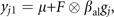 where μ is the grand mean, F is a full matrix v by 1 containing the estimated factor loadings, βal is a 1 by 1 matrix containing the estimated allelic effect and gj represents the genotype of individual j, coded as the number of reference alleles at the locus minus 1.
 -
The second, alternate, model of the mean effects allows for variable-specific association at the level of the individual trait:
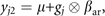 where βar is a v by 1 matrix containing the estimated allelic effects for each of the k phenotypes.
 -
The null model yj0=μ, in which no association effects are estimated.
 where μ is the grand mean, F is a full matrix v by 1 containing the estimated factor loadings, βal is a 1 by 1 matrix containing the estimated allelic effect and gj represents the genotype of individual j, coded as the number of reference alleles at the locus minus 1.
 where βar is a v by 1 matrix containing the estimated allelic effects for each of the k phenotypes.
The minus twice log-likelihoods of the two alternate models are compared with the null model using likelihood ratio χ2-test with degrees of freedom equal to the number of parameters being tested; one in the case of the factor-level test (χ21) and v for the variable-specific test (χν2). As the two tests provide complementary information, it is suggested that the results of both tests should be reported. As discussed below, conducting both factor-level and variable-specific tests results in an inflated type I error rate, which may be corrected by applying a Bonferroni correction to the factor-level and variable-specific tests. Adjusted P-values may be obtained by multiplying the observed P-values, by the Bonferroni correction factor.
In the case of family data, allelic effects may be partitioned into between (βb) and within (βw) family effects at either the latent or variable-specific level (eg βbal and βbar).3 For a test of association robust to population stratification, the within-family test may be used, in which case these three models may be parameterized as follows, for the jth sib from the ith family:

where Abi is the derived coefficient for the between-families additive genetic effect for the ith family, and Awij is the coefficient for the within-families additive genetic effect for the jth sib from the ith family, as summarized in Table 1. Alternatively, in the absence of population stratification, a between-families test in which the βw parameters are constrained to equal the βb parameters may be used, in which case:

Simulations studies
To examine the type I error and power of the combined multivariate (CMV) approach, data were simulated in R under nine scenarios. In each scenario, covariation between variables was due to a single factor, which loaded on all variables. Algebraically, this covariation may be written as F*F′, where F is a full matrix v by 1, where v is the number of variables. Uncorrelated residuals were added as D*D′, where D is a v by v diagonal matrix. The factor loadings and residuals for each scenario are summarized in Table 2. Data from unrelated individuals (N=1000) were simulated for six (a–f) scenarios; in the remaining three (g–i), data for full sib-pairs (Npairs=1000) were simulated.
Data for each of the nine scenarios were simulated under six association models: (1) Null effect (to assess type I error); (2) single-variable association; (3) factor-level association; (4) residual-level association in which all variables are equally associated; (5) a mixed effects model and (6) a contrasting effects model. A total of 5000 replicates were simulated for each association model using a single SNP (single nucleotide polymorphism) with a 0.2 minor allele frequency throughout.
To compare the power of the CMV approach to univariate analyses of factor scores or sum scores (SSs), we computed the following: a SS; a ‘regression’ (aka Thompson) factor score,4 in which the sum of squared discrepancies between true and estimated factors over individuals is minimized and a ‘Bartlett’ factor score (BFS),5, 6 in which the sum of squares of the unique factors over the range of items is minimized. Using the raw multivariate data for each replicate, we ran the CMV association test and univariate association tests of (i) the SS, (ii) the Bartlett and (iii) the regression factor scores (RFS). For the sibling data from scenarios g–i, a between-families test of association was used.
To examine the effect of missing phenotypic data on the power of the CMV approach, two additional conditions were investigated using data simulated under the parameters from scenario i. In the first simulation, 10% of the data for each variable were set to missing. Missing status was randomly assigned across individuals and variables. In the second simulation, the third variable was randomly set to missing for half of the participants to mimic a situation in which not all participants were assessed on all variables. Each of these missing data scenarios was simulated for unrelated individuals under the single-variable and factor-level association models (described in association models 2 and 3 in Table 2). A total of 5000 replicates were simulated for each case using a single SNP with a 0.2 minor allele frequency. Although the effects of missingness are not exhaustively explored, it is expected that the results of these simulations will generalize to other situations in which data is missing at random (and missing completely at random), including the case of sib-pairs in which missingness may be correlated.
All analyses were conducted using Mx,7 a freeware structural equation modeling program. The scripts used in these analyses are available from (www.vipbg.vcu.edu/~sarahme/WriteMx) and may be modified to explore other conditions.
Applied example
To illustrate the explanatory strengths of the CMV approach, we applied it to data from the National Longitudinal Study of Adolescent Health (Add Health; http://www.cpc.unc.edu/AddHealth). This nationally representative longitudinal study is designed to assess the causes and consequences of health-related behaviors of adolescents initially recruited in grades 7 through 12 as they transition into adulthood.
During the third wave of data collection (2001–2002), saliva samples were collected, which were used to genotype polymorphisms in the dopamine receptor D2 (DRD2) TaqIA snp (dbSNP rs1800497; g.32806C>T; 11q23; OMIM *126450; for details of the sample processing and genotyping see Haberstick and Smolen8). The DRD2 Taq1A1 (T) allele has been associated with a range of substance use phenotypes including alcoholism,9, 10 nicotine use and cessation.11, 12, 13 In addition, the degree of pleasure gained from the effects of psychostimulants has been found to correlate with the density of dopamine D2 receptors in the striatum,14 which is in turn associated with DRD2 Taq1A1.15 In this study, we consider association between the DRD2 TaqIA polymorphism and initiation (ever-use) of three substances: marijuana, tranquilizers and stimulants, using data from 864 Caucasian males.
The characteristics of the sample are summarized in Table 3. The phenotypic data were analyzed employing a multifactorial threshold model, which specifies that ordinal data represent subdivisions on an underlying normal distribution of liability.16
Results
Type I error
As shown in Table 4, across scenarios the factor-level and variable-specific tests showed the expected type I error rates for when considered individually. The distributions of the P-values for the factor-level and variable-specific tests were uniform (see Supplementary Figures 1–4). The CMV approach resulted in an inflated type I error, mean α=0.084. To control for this inflation in type I error rates, we adopted an α level of 0.025 for each of the factor-level and variable-specific tests, which resulted in a slightly conservative test, mean α=0.043. This reduced α level was used in all further analyses. The conservative nature of the CMV approach is due to the covariation between the factor-level and variable-specific tests. However, as the magnitude of this covariation is dependent on the factor structure of the observed data, researchers may either estimate an exact Bonferroni correction for their data through permutation or simulation, or adopt the slightly conservative α level of 0.025.
Power
Figures 1a–c summarize the results of the power analyses for the five association models under the nine multivariate scenarios. In each case, power is shown for the CMV approach and for univariate analyses of the SS (SS), RFS and BFS.


(a) Power to detect association (defined as the proportion of tests significant at an α of 0.05) under multivariate backgrounds a, b and c, for association models 2–6 (described in Table 2). In each case power is shown for the Combined multivariate approach (CMV) and for univariate analyses of the sum score (SS), Regression factor score (RFS) and Bartlett factor score (BFS). (b) Power to detect association under multivariate backgrounds d, e and f, for association models 2–6. (c) Power to detect association under multivariate backgrounds g, h and i, for association models 2–6.
The situations in which the association affected all variables, either at the factor level (association model 3) or to an equal extent across all variables (association model 4), all the four association tests performed well. In these scenarios, the slightly conservative nature of the α correction for the combined tests is evident as a slight loss of power, which is most obvious when the factor loadings are high. However, the power of the sum and factor score analyses decreases sharply as the pattern of association effects diverges from that of the factor loadings (association model 2, 5 and 6). This effect is seen most clearly in contrasting effects simulations (association model 6), in which the direction of association differs between variables. For the univariate analyses of the sum and factor scores, the power to detect this type of allelic effect is very low and often does not differ from chance. This is consistent with previous work that has shown that multivariate linkage analyses are most powerful when the covariation induced by a QTL differs in direction from the background correlation.17
As might be expected, of the three univariate analyses, the SS was the least powerful across situations, whereas the BFS outperformed the RFS. Conversely, across the range of situations considered here, the CMV approach is robust and generally has equal or greater statistical power than the univariate analyses of summary measures. As shown in Table 5, an overall missingness rate of 30% resulted in an approximate 4.5% reduction in power (from 0.922 to 0.879 for the single variable association and 0.775 to 0.740 for the factor-level association). However, when the ‘true’ association effect was at the level of the factor, a substantial missingness (50% of variable 3) had only a minor impact on the power to detect association, resulting in a reduction in power of ∼1% (0.775 vs 0.769).
Applied example
To show the CMV approach, we analyzed association between the DRD2 TaqIA polymorphism and initiation (ever-use) of three substances – marijuana, tranquilizers and stimulants – using data from 864 Caucasian males. Marijuana, tranquilizer and stimulant initiation were moderately correlated and all three loaded strongly on a common factor (Table 3). There was no evidence of factor-level association (χ12=0.65, βFactor=0.06). However, a significant association was observed at the variable-specific level (χ32=13.91; α=0.025; Pcorrected=0.006; βStimulants=−0.19, βTranquilizers=0.14, βMarijuana=0.11). These results suggest that the T-allele increases the risk of stimulant use, but decreases the risk of tranquilizer and marijuana use, which is consistent with the patterns of prevalence by genotype shown in Table 3. Interestingly, in these data the differences in the direction of the allelic effects at the variable-specific level cancel each other out at the factor level. To determine whether these results would have been evident from univariate analyses, we conducted post-hoc analyses of each variable. The association between stimulant use and DRD2 was nominally significant (at the 0.05 level) before correcting for multiple testing (χ12=3.88, P=0.049, β=−0.18). However, there was no evidence for association with either tranquilizer (χ12=1.65, β=0.13) or marijuana use (χ12=2.60, β=0.11), and none of the univariate tests of association for the different drugs would remain significant following Bonferroni correction. The increase in power associated with the multivariate analysis within an association framework is analogous to that observed in linkage.17, 18
These results may seem counterintuitive given the published reports9, 12, 19 that the DRD2 A1 (T) allele is a risk allele for a range of different substance use phenotypes and that the majority of covariation in substance use phenotypes can be explained by common etiological factors. However, the effects of stimulants (including elevated activity, mood and euphoria) are markedly different from those of tranquilizer and marijuana use (which typically include relaxation, lethargy, mild euphoria and anxiety-reduction). To the extent that individuals with higher D2 receptor density, which is associated with DRD2 Taq1A1 (T-allele),15 are more likely to report the effects of a psychostimulant drug (methylphenidate which, like cocaine, blocks the dopamine transporters) as unpleasant,14 it is possible that individuals with T-alleles may be more likely to try drugs that are perceived to increase exhilaration and animation than those that are thought to have the opposite effect. Although this association has yet to be replicated, the finding illustrates the increased explanatory power of the CMV approach.
Discussion
Although univariate analysis of a factor score can detect an association at the factor level and univariate analyses of each phenotype in turn may detect allelic effects, the need to correct for multiple testing is disadvantageous. Furthermore, such a procedure does not exploit the gain in power derived from multivariate analysis. The suitability of the current approach to some extent depends on the phenotypes under analysis. The performance exceeds that of alternatives when the phenotypic covariance arising from other genetic and environmental influences differs from that generated by the QTL.17 We expect that the multivariate approach will prove useful in the analysis of complex traits that involve behavioral, psychological or other factors that are inherently difficult to measure. It should be especially valuable when analyzing data that contain missing values, perhaps due to a structured data collection format, or when a subsample has been chosen for more detailed or expensive assessments. Extension of the method to factor mixture models would provide a natural framework for the analysis of traits such as migraine and ADHD, in which symptom patterns suggest the presence of subtypes. The framework is directly suitable for repeated measures of either one trait or many, and can be used in situations in which there is measurement non-invariance.20, 21
To facilitate application of the CMV approach, we have developed a perl script, which can be downloaded from (www.vipbg.vcu.edu/~sarahme/WriteMx). This script can be used with either family or individual data. It reads standard Merlin .ped and .dat files, and writes a data file and customized scripts for running the analysis in Mx (which can be freely downloaded for a range of operating systems http://www.vcu.edu/mx/). Mx allows full user specification; as such the approach described here can easily be extended to allow for analysis of multiple factors, and scripts showing this extension can be downloaded from (www.vipbg.vcu.edu/~sarahme/WriteMx). In addition, the method can be extended to accommodate data from different types of relatives (parents, grandparents etc).
The current implementation within Mx has some limitations. It is not presently possible to impute missing genotypes within the CMV approach, and at present individuals with missing genotypes will be excluded from the analysis. However, pre-imputed genotypes can easily be analyzed within Mx, and information regarding the precision of imputation can be incorporated through the use of mixture modeling. In addition, Mx can analyze either continuous or ordinal (binary and/or polychotomous) data. However, there is no straightforward general approach to the joint analysis of binary and continuous variables in the current version of Mx, although it is practical to do this when the number of patterns of missing continuous variables is small. An R-language Open Source version of the software, currently under development, will implement this functionality directly. In the meantime, one solution to this problem is to transform continuous variables to ordinal, using deciles and conduct a multivariate ordinal analysis.
To summarize, this article has three main contributions. First, it introduces an integrated model for allelic association, which permits testing for association to either a common factor or to a set of variable-specific components. The approach improves the explanatory power of analysis, analogous to that derived from using pathway-based association approaches to complement traditional single SNP analysis.22 Second, it presents freely available software that facilitates the use of the combined association approach by producing scripts and data for Mx analysis from Merlin format ped and dat files. Third, it illustrates the approach using substance use data from the Add Health study. We encourage researchers to look beyond diagnosis or SS analyses when working with complex traits in the hope that doing so will lead to the identification of novel susceptibility genes and a deeper understanding of the ways in which identified variants influence behavior and complex traits.
References
Lange C, van Steen K, Andrew T et al: A family-based association test for repeatedly measured quantitative traits adjusting for unknown environmental and/or polygenic effects. Stat Appl Genet Mol Biol 2004; 3: Article 17. http://www.ncbi.nlm.nih.gov/pubmed/16646795?ordinalpos=1&itool=EntrezSystem2.PEntrez.Pubmed.Pubmed_Results Panel.Pubmed_DefaultReportPanel.Pubmed_RVDocSum.
Lange C, Silverman EK, Xu X, Weiss ST, Laird NM : A multivariate family-based association test using generalized estimating equations: FBAT-GEE. Biostatistics 2003; 4: 195–206.
Fulker DW, Cherny SS, Sham PC, Hewitt JK : Combined linkage and association sib-pair analysis for quantitative traits. Am J Hum Genet 1999; 64: 259–267.
Thomson GH : The Factorial Analysis of Human Ability. London: London University Press, 1951.
Bartlett MS : The statistical conception of mental factors. Br J Psychol 1937; 141: 97–104.
Bartlett MS : Methods of estimating mental factors. Nature 1938; 28: 609–610.
Neale MC, Boker SM, Xie G, Maes HH : Mx: Statistical Modeling; VCU Box 900126, Richmond, VA 23298 http://www.vcu.edu/mx/ Department of Psychiatry, 2006.
Haberstick BC, Smolen A : Genotyping of three single nucleotide polymorphisms following whole genome preamplification of DNA collected from buccal cells. Behav Genet 2004; 34: 541–547.
Dick DM, Wang JC, Plunkett J et al: Family-based association analyses of alcohol dependence phenotypes across DRD2 and neighboring gene ANKK1. Alcohol Clin Exp Res 2007; 31: 1645–1653.
Smith L, Watson M, Gates S, Ball D, Foxcroft D : Meta-analysis of the association of the Taq1A polymorphism with the risk of alcohol dependency: a HuGE gene-disease association review. Am J Epidemiol 2008; 167: 125–138.
David SP, Strong DR, Munafo MR et al: Bupropion efficacy for smoking cessation is influenced by the DRD2 Taq1A polymorphism: analysis of pooled data from two clinical trials. Nicotine Tob Res 2007; 9: 1251–1257.
Munafo M, Clark T, Johnstone E, Murphy M, Walton R : The genetic basis for smoking behavior: a systematic review and meta-analysis. Nicotine Tob Res 2004; 6: 583–597.
Ton TG, Rossing MA, Bowen DJ, Srinouanprachan S, Wicklund K, Farin FM : Genetic polymorphisms in dopamine-related genes and smoking cessation in women: a prospective cohort study. Behav Brain Funct 2007; 3: 22.
Volkow ND, Wang GJ, Fowler JS et al: Prediction of reinforcing responses to psychostimulants in humans by brain dopamine D2 receptor levels. Am J Psychiatry 1999; 156: 1440–1443.
Jonsson EG, Nothen MM, Grunhage F et al: Polymorphisms in the dopamine D2 receptor gene and their relationships to striatal dopamine receptor density of healthy volunteers. Mol Psychiatry 1999; 4: 290–296.
Neale MC, Cardon LR : Methodology for genetic studies of twins and families. Dordrecht, The Netherlands: Kluwer Academic Publishers, 1992.
Evans DM : The power of multivariate quantitative-trait loci linkage analysis is influenced by the correlation between variables. Am J Hum Genet 2002; 70: 1599–1602.
Boomsma DI, Dolan CV : A comparison of power to detect a QTL in sib-pair data using multivariate phenotypes, mean phenotypes, and factor scores. Behav Genet 1998; 28: 329–340.
Noble EP, Blum K, Khalsa ME et al: Allelic association of the D2 dopamine receptor gene with cocaine dependence. Drug Alcohol Depend 1993; 33: 271–285.
Lubke GH, Dolan CV, Neale MC : Implications of absence of measurement invariance for detecting sex limitation and genotype by environment interaction. Twin Res 2004; 7: 292–298.
Meredith W : Measurement invariance, factor analysis, and factorial invariance. Psychometrika 1993; 58: 525–543.
Wang K, Li M, Bucan M : Pathway-based approaches for analysis of genomewide association studies. Am J Hum Genet 2007; 81: 1278–1283.
Acknowledgements
This research uses data from Add Health, a program project designed by J Richard Udry, Peter S Bearman and Kathleen Mullan Harris, and funded by a grant P01-HD31921 from the Eunice Kennedy Shriver National Institute of Child Health and Human Development, with cooperative funding from 17 other agencies. Special thanks is due to Ronald R Rindfuss and Barbara Entwisle for assistance in the original design. Persons interested in obtaining data files from Add Health should contact Add Health, Carolina Population Center, 123 W. Franklin Street, Chapel Hill, NC 27516-2524 (Add Health@unc.edu). No direct support was received from grant P01-HD31921 for this analysis. SEM is supported by an Australian NHMRC Sidney Sax fellowship (443036). This work was supported by a NIDA MERIT Award (DA-018673) to MCN. Statistical analyses were carried out on the Genetic Cluster Computer (http://www.geneticcluster.org) which is financially supported by the Netherlands Scientific Organization (NWO 480-05-003).
Author information
Authors and Affiliations
Corresponding author
Additional information
Supplementary Information accompanies the paper on European Journal of Human Genetics website (http://www.nature.com/ejhg)
Supplementary information
Rights and permissions
About this article
Cite this article
Medland, S., Neale, M. An integrated phenomic approach to multivariate allelic association. Eur J Hum Genet 18, 233–239 (2010). https://doi.org/10.1038/ejhg.2009.133
Received:
Revised:
Accepted:
Published:
Issue Date:
DOI: https://doi.org/10.1038/ejhg.2009.133
Keywords
This article is cited by
-
Powerful and Efficient Strategies for Genetic Association Testing of Symptom and Questionnaire Data in Psychiatric Genetic Studies
Scientific Reports (2019)
-
A Fast Method for Estimating Statistical Power of Multivariate GWAS in Real Case Scenarios: Examples from the Field of Imaging Genetics
Behavior Genetics (2019)
-
Heritability of Behavioral Problems in 7-Year Olds Based on Shared and Unique Aspects of Parental Views
Behavior Genetics (2017)
-
GW-SEM: A Statistical Package to Conduct Genome-Wide Structural Equation Modeling
Behavior Genetics (2017)
-
Multivariate Gene-Based Association Test on Family Data in MGAS
Behavior Genetics (2016)
