
Abstract
In this feasibility study we propose a method based on sodium magnetic resonance imaging (MRI) for estimating simultaneously the intracellular sodium concentration (C1, in mM) and the extracellular volume fraction (α) in grey and white matters (GM, WM) in brain in vivo. Mean C1 over five healthy volunteers was measured ~11 mM in both GM and WM, mean α was measured ~0.22 in GM and ~0.18 in WM, which are in close agreement with standard values for healthy brain tissue (C1 ~ 10–15 mM, α ~ 0.2). Simulation of ‘fluid’ and ‘solid’ inclusions were accurately detected on both the C1 and α 3D maps and in the C1 and α distributions over whole GM and WM. This non-invasive and quantitative method could provide new biochemical information for assessing ion homeostasis and cell integrity in brain and help the diagnosis of early signs of neuropathologies such as multiple sclerosis, Alzheimer's disease, brain tumors or stroke.
Introduction
Magnetic resonance imaging (MRI) is a powerful tool for imaging the body in vivo and diagnosing a large range of diseases in practically all parts of the human body. Standard MRI is based on the detection of protons (1H) present in water, lipids and macromolecules in the body. It can generate a wide range of different contrasts (such as proton density, T1-weighted, T2-weighted, diffusion, perfusion, blood-oxygen level dependent, etc.) giving different anatomical, structural, or sometimes functional, information on the tissues under investigation1. However, standard MRI is generally not quantitative and cannot provide direct biochemical information on tissue viability (such as homeostasis or cell membrane integrity). This kind of information could be of upmost importance for diagnosing and prognosing diseases, or for assessing the effect of treatments and new drug tests. In the present feasibility/proof of concept study, we propose using a simple method based on sodium MRI2 for measuring simultaneously two tissue parameters, intracellular sodium concentration (called C1 in this study) and extracellular volume fraction (α), in brain in vivo in a quantitative and non-invasive manner on a clinical 3 T scanner. These two parameters are very sensitive to cell viability and ion homeostasis2,3,4 and could therefore be used as biomarkers of neurodegenerative diseases for measuring early impairment in energy production or membrane integrity before any sign can be detected with standard imaging techniques. Measuring changes in extracellular volume fraction would give information on effusion or disruption of cell packing5, dehydration6, changes in vascularization or tumor edema angiogenesis7,8 or even metabolite clearance in the brain9. Measuring changes in intracellular sodium concentration would help assess the degree of cell hypometabolism or injury3, tumor malignancy10,11 or resistance to therapy12.
Sodium is a vital component of the human brain and sodium ion (23Na+) homeostasis is a major process in cells through coupled exchange with potassium ions (K+) between intra- and extracellular spaces using the Na+/K+-ATPase (sodium-potassium pump)13. This pumping process maintains a constant gradient of concentrations across the membrane (10–15 mM intracellular versus 140 mM extracellular) which is used to control cell volume, pH balance, glucose and neurotransmitter transport, calcium regulation, membrane electrical potential (and therefore nerve pulse transmission) and protect the cell from bursting as a result of osmotic swelling. This process is very energy-consuming and is therefore very dependent on adenosine triphosphate (ATP) production and hydrolysis in cells. Regulation of Na+/K+-ATPase therefore plays an essential role in the etiology of brain pathologies. Dysregulation of the Na+/K+-ATPase or impairment of ATP-dependent processes will provoke a loss of Na+ homeostasis and therefore increase of intracellular sodium concentration (as the gradient cannot be maintained anymore) leading ultimately to cell death (and concomitant increase of extracellular volume fraction). Being able to estimate quantitatively both C1 and α in brain in vivo could therefore provide fundamental new metabolic information for detecting early processes of loss of cell integrity in both acute diseases such as stroke14 and chronic diseases such as brain tumors15,16, multiple sclerosis17 or Alzheimer's disease18. This biochemical information could be combined with anatomical proton MRI (for measuring structural changes in brain) or positron emission tomography (PET, for measuring glucose consumption for example), in order to assess the prognosis of pathologies and their response to new treatments.
Sodium MRI is based on the detection of Na+ ions present in different concentrations in tissues2,19,20. Sodium ion has a quadrupolar nucleus of spin 3/2 that yields the second strongest nuclear magnetic resonance (NMR) signal among all nuclei present in biological tissues, after proton 1H. The average sodium concentration in brain is around 40 mM if we take into account the average extra- and intracellular volume fractions (about 0.2 and 0.6 respectively, with solid volume fraction ~0.2) in brain. The NMR sensitivity of sodium is 9.27% of the proton sensitivity, which combined with low concentrations compared to water protons (110 M, for 2 protons/water molecule), leads to an average sodium NMR signal about 30,000 times lower than proton signal in brain. Moreover, due to their quadrupolar moment, sodium spins interact very strongly with the electric field gradients of their surroundings, leading to very short relaxation times in tissues (with monoexponential T1 ~ 30–40 ms and biexponential T2short ~ 1–5 ms and T2long ~ 15–30 ms in brain) compared to protons. Because of all these parameters, sodium MRI can be accomplished using high magnetic fields (≥3 T), ultrashort echo time (UTE) acquisition sequences and with low resolution (≥4 mm). Many averages are also necessary for increasing the signal-to-noise ratio (SNR) of the images, but this leads to long acquisition times (10–20 min). Thanks to recent advances in hardware capabilities such as high fields and strong stable magnetic gradients, sodium MRI is can now be implemented on many clinical scanners provided some specific hardware and software is installed (amplifiers, dual-tuned 1H/23Na radiofrequency coils, non-Cartesian UTE sequences and reconstruction algorithms). Previous studies have suggested the use of sodium MRI for assessing intracellular sodium and extracellular or intracellular volume but did not implemented it completely19, or used the more complicated triple quantum filters (TQF)21. TQF acquisitions necessitate higher magnetic fields (7 T), are more sensitive to radiofrequency (RF) and static magnetic field inhomogeneities22,23 and previous studies did not separate grey and white matters (GM, WM) in brain.
We propose here a simple sodium MRI method that can be applicable on a clinical 3 T scanner, which can generate simultaneously C1 and α 3D maps and their respective distributions in GM and WM separately. Data quantification can be performed by using a combination of five calibration phantoms with known sodium concentrations and relaxation times placed within the field-of-view (FOV) of the images and two major steps. The first step consists of calculating the apparent total sodium concentration (aTSC) and apparent intracellular sodium concentrations (aISC) maps from two sodium MRI acquisitions: one simple full sodium acquisition and one with fluid suppression by inversion recovery (IR)16,24,25, respectively. Using masks of grey matter and white matter from double inversion recovery (DIR) proton MRI with turbo spin echo acquisition26,27,28, we can obtain aTSC and aISC maps of GM and WM separately. See Figure 1 for a description of this process. The second step consist of calculating the C1 and α maps in GM and WM from aTSC and aISC in combination with a simple three-compartment model (intracellular, extracellular and solid compartments) as shown in Figure 2. The full data processing is described in more details in the Methods section.

Diagram of the brain MRI data processing.
The process is divided in five steps: (1) 23Na data acquisition with and without fluid suppression by IR and 1H data DIR acquisition; (2) Linear regression from the 23Na signal of the five calibration phantoms; (3) Calculation of the apparent total and intracellular sodium concentration maps (aTSC and aISC) from the linear regression; (4) Calculation of the GM, WM and full brain (GM + WM) masks from the DIR data using SPM8; (5) Multiplication of the sodium maps by the masks.

Three-compartment model.
In this simple model, we assume that each voxel can be separated in three compartments. Compartment 1 corresponds to the intracellular volume V1 (in L) of sodium concentration C1 (in mmol/L, or mM). Compartment 2 corresponds to the extracellular volume V2 of sodium concentration C2. These two compartments correspond to the total fluid space of the model. Compartment 3 of volume Vs corresponds to all the ‘solid’ components within the voxel (cell membranes and nuclei, proteins and other metabolites), where sodium content is negligible. The total volume is Vt = V1 + V2 + Vs. Unknown values of interest are the intracellular sodium concentration C1 and the extracellular volume fraction α. In this model, we consider that the extracellular sodium concentration is constant and known C2 ~ 140 mM and that the fluid (or water) volume fraction w is also known (w ~ 0.7 in WM, w ~ 0.85 in GM).
Results
Extracellular volume fraction and intracellular sodium concentration quantification in vivo
Examples of extracellular volume fraction (α) maps and intracellular sodium concentration (C1) maps from one volunteer are shown in Figure 3. Examples of the distributions of C1 and α values from the same volunteer, over the whole 3D data for WM, GM and full brain (GM + WM) are shown in Figure 4. Table 1 summarizes the mean and standard deviation of different statistical parameters of the C1 and α distributions over all volunteers (n = 5). The mean value of the mean, median and mode of C1 measured with this method is around 11 ± 2 mM in both GM and WM, with mean standard deviation about 6 ± 0.2 mM. These values match closely the usual values in healthy brain found in the literature, which are generally in the range 10–15 mM20,29. The mean value of mean α was measured around 0.22 ± 0.04 in GM and 0.18 ± 0.05 in WM, which is also in close agreement with its standard average value in brain (α ~ 0.2) measured in different mammal brains with diffusion techniques8. Moreover, standard error (or uncertainty) propagation30 was calculated for typical and extreme variations of the parameters (aTSC, aISC, water fraction w and extracellular/CSF sodium concentration C2) used to calculate C1 and α. See Methods and Supplementary Information, for details. Main results are shown in Table 2. In summary, an uncertainty of around 5 mM (36%) and 0.06 (32%) can be expected when measuring C1 and α, for typical variations in water content, extracellular (or CSF) sodium concentration and errors in data processing of aTSC and aISC due to noise or incomplete fluid suppression by inversion recovery.

Intracellular sodium concentration (C1) and extracellular volume fraction (α) maps of the brain of a healthy volunteer (1 axial slice).
(a) C1 of full brain (GM + WM), (b) C1 of GM, (c) C1 of WM, (d) α of full brain (GM + WM), (e) α of GM, (f) α of WM.

Distribution of all intracellular sodium concentration (C1) values and all extracellular volume fraction (α) values in full brain (GM + WM, black), GM (blue), WM (red) from a volunteer.
(a) C1 in full brain, (b) C1 in GM, (c) C1 in WM, (d) α in full brain, (e) α in GM, (f) α in WM. Statistical parameters of the distributions are included in the top right corner of each histogram. Pixel number is given in % of the total number of pixels in full brain, in GM and in WM, respectively. Abbreviations: Std = standard deviation, Min = minimum, Max = maximum, Skew = skewness, Kurt = kurtosis.
Interestingly, both C1 and α distributions exhibit non-zero skewness (which quantifies how asymmetrical the distribution is) and kurtosis (which quantifies how the shape of a distribution matches the Gaussian distribution)31. All volunteers exhibit similar skewness and kurtosis. An average skewness of ~0.4 was measured for C1 in WM and GM, ~0.9 for α in WM and ~1.4 for α in GM: both distributions from normal brains are skewed towards higher values (right side). An average kurtosis of ~4 for C1 in WM and GM and ~4.5 for α in GM and ~8 in WM, can be interpreted as a more ‘peaked’ distribution compared to a Gaussian.
Simulations
Simulation of artificial ‘fluid’ or ‘solid’ inclusions in the brain were investigated for testing the effectiveness of the method for detecting abnormalities in the brain. The ‘fluid’ inclusion (cystic fluid-type) was simulated by adding a 10 × 10 × 10 voxels inclusion in the brain region (mostly GM) of the aTSC and aISC maps, with aTSC = 120 mM (very high total sodium content compared to normal 30–40 mM) and aISC = 5 mM (low apparent intracellular sodium compared to normal 10–15 mM), prior to C1 and α quantification. For the ‘solid’ inclusion (tumor-type), aTSC = 55 mM (high total sodium content) and aISC = 25 mM (high intracellular sodium content). Noise in the range [−2,2] mM was also added to the aISC and aTSC values of the inclusion for a more realistic simulation of noisy sodium data. These inclusions represent about 1.15% of the total brain volume (1000 voxels over 86571 voxels in whole GM + WM). The corresponding C1 and α maps and distributions are shown in the supplementary figures S1–S2 (‘fluid’) and S3–S4 (‘solid’). The ‘fluid’ inclusion is very distinct on the α map with a mean value ~0.8 compared to normal brain with α ~ 0.2 and appears dark on the C1 map with a mean value = 0. This ‘fluid’ inclusion can also be easily detected on the α distributions in full brain, WM and GM as an additive peak around 0.8. Note that the mean, median and mode of α remain practically unchanged compared to average values from normal brain, but that the skewness and kurtosis are greatly increased by factors ~3 and ~4 respectively. The ‘solid’ inclusion appears very distinctively on the C1 map with a mean value ~45 mM compared to normal brain with C1 ~ 10–15 mM and is undetectable on the α map with a mean value = 0.2. This ‘solid’ inclusion can also be easily detected on the C1 distributions in full brain, WM and GM as an additive peak around 40–50 mM. Note that the mean, median and mode of C1 remain practically unchanged compared to average values from normal brain, but that the skewness and kurtosis are increased by factors ~2–4 and ~2–3 respectively.
Discussion
Mean values for both C1 and α estimated with this simple sodium MRI method (2 acquisitions) and simple model (three-compartment) are in close agreement with standard values measured in healthy brain tissue. In all five volunteers, we found that the mean α in WM (~0.18) was lower than in GM (~0.22), but no conclusion can be drawn for the moment as our sample size is too small. Most of literature gives an average α ~ 0.2 in brain, without distinction between GM and WM5,8. More healthy subjects will be scanned for assessing the repeatability, reproducibility and robustness in estimating C1 and α of the method prior to application to patients with neuropathologies. The robustness of the method is closely dependent on the sodium quantification using calibration phantoms, as a slight change in the slope of the linear regression function can induce large variations in the aISC and aTSC maps. In our model, we therefore calculated the aISC and aTSC maps only when the signal from the calibration phantoms was fitted by linear regression with the condition that both coefficients of determination R2 > 0.99 and adjusted R2adj > 0.98 (which takes into account the number of variables and sample size). This condition held every time and is the norm. Only on one subject the values of R2 and R2adj were slightly below the thresholds (0.98 and 0.97 respectively), due to malposition of the gels next to the head.
From the uncertainties calculation (error propagation), variations of C1 and α due to uncertainties in aTSC and aISC calculation (due to noise or imperfect inversion) and in estimation of w and C2, are within the range of the mean standard deviations (about 6 mM and 0.08, respectively) that we measured on the volunteers (see Table 1). This indicates that this method would be able to detect changes in C1 and α of above 40% (C1 > 20 mM and α > 0.28) in pathologies, which are of the order of changes expected from the literature5,6,7,8,9,10,11,12.
Both C1 and α distributions had positive skewness and kurtosis in WM and GM, which can be interpreted from both (1) a methodological and (2) a biophysical a point-of-view. (1) The sodium images were acquired with low resolution (5 and 6.7 mm isotropic), which generates large partial volume effect, mainly in the regions close to the ventricles and subarachnoid space (filled with cerebrospinal fluid - CSF). Sodium images were then reconstructed with a nominal resolution of 2.5 mm matching DIR MRI and then multiplied by the GM and WM masks. The masked sodium data contained therefore remnant partial volume effect from the presence of CSF in some voxels with high extracellular volume fraction. This leads to an increase in the number of voxels with high values in the α map and low intracellular sodium concentration and therefore to an increase of the number of C1 values close to zero, affecting both skewness and kurtosis. Moreover, as sodium images have low signal-to-noise ratio (SNR ~ 25–30 and ~10–15 for acquisitions without and with IR, respectively), noise can also be an important factor in the skewness and kurtosis of the distributions. (2) From a biophysical point-of-view, WM and GM have different structures and cell packing characteristics32 that can greatly influence the distributions of C1 and α. It is generally admitted that WM, which consists mainly of axons and glial cells, has a more anisotropic structure than GM32,33, associated with a wider (with thicker tails) distribution of extracellular volume fractions (higher kurtosis) while keeping the similar intracellular sodium concentration distributions (C1 skewness and kurtosis are very similar in GM and WM).
For testing the effectiveness of the proposed method for detecting pathologies in brain, two artificial ‘fluid’ (cyst-type) and ‘solid’ (tumor-type) inclusions were added to the aTSC and aISC maps with values representing the potential increase of sodium content in these regions. Both inclusions, representing around 1% of change in total brain volume, were well defined and differentiated in both the C1 and α maps and distributions. Moreover, we could see on the C1 and α distributions that the mean values were not changed by the inclusions, but that the skewness and kurtosis were significantly different. This artificial model is of course too simple to model real pathologies, which are much more complex than simply ‘fluid’ or ‘solid’. We nevertheless think that, as a first approximation for this exploratory study, it is reasonable to expect that cystic-type pathologies will have C1 and α leaning towards fluid-type values, while tumor-like pathologies (such as neoplasms) will have C1 and α leaning towards solid-type values. Testing the proposed method on patients with different pathologies is under planning and will help assess the accuracy and potential applicability of this method and help refine the model as necessary.
In conclusion, we have developed a non-invasive and quantitative technique based on a simple model, two sodium and two proton MRI acquisitions for estimating the intracellular sodium concentration and extracellular volume fraction in cerebral WM and GM in vivo, on a clinical 3 T scanner. Future work will include a more complete model (multi-compartment model including also interstitial space, vascular space, CSF), new RF dual-tuned multichannel RF coil, optimized acquisition sequence and reconstruction. This latter part will include compressed sensing (CS)34 or denoising techniques35, for improving SNR of the sodium images, reduce the acquisition time and/or increase the resolution. This would allow to acquire more sodium images with different inversion recovery times for improving the accuracy and robustness of the technique. In the case of compressed sensing, there is no need of using a random distribution of interleaves as FLORET already has low coherence (and therefore undersampling artifacts add incoherently to the sparse signal coefficients). Undersampling the outer part of the FLORET k-space leads to a reduction of interleaves needed to fill the k-space but at a loss of resolution and induced blurring. Applying CS reconstruction might help for increasing the resolution and denoising the data. In the end, applying CS would allow (if successful) to: (1) increase the SNR while keeping the same acquisition time and same resolution, or (2) reduce the acquisition time while keeping the same SNR and same resolution, or (3) help increase the resolution of the images while compensating for the loss of SNR.
Moreover, as the fluid fraction (w) in brain also changes with pathologies, future work will also include techniques for estimating the local water content36 which will be included in the new model (and not considered constant anymore).
Methods
MRI human subjects
The brains of five healthy subjects (3 males, 2 females, mean age = 33 ± 7 years) were scanned after approval from the Institutional Review Board of the New York University Langone Medical Center and signed inform consent. The methods were carried out in accordance with Food and Drugs Administration (FDA) guidelines.
MRI hardware
The MRI experiments were performed on a 3T Tim trio system (Siemens, Erlangen, Germany) using a dual-tuned 1H/23Na birdcage radiofrequency coil tuned at 128/33 MHz (Stark Contrast, Erlangen, Germany).
Proton MRI acquisitions
Two double inversion recovery (DIR) 1H MRI acquisitions were performed. The first DIR image was acquired in order to suppress both CSF and WM using the DIR Turbo Spin Echo SPACE sequence28,37 with the following parameters: TR = 7500 ms, TE = 300 ms, field-of-view (FOV) = 220 × 320 × 320 mm3, resolution = 2.5 mm isotropic, inversion times TI1 = 2650 ms and TI2 = 550 ms, time of acquisition (TA) = 4:00 min. The second DIR image was acquired in order to suppress both CSF and GM with the same parameters as the first DIR except TI1 = 2800 ms and TI2 = 800 ms.
Sodium MRI acquisitions
Sodium acquisitions were performed using the 3D UTE non-Cartesian FLORET sequence38 with the following parameters:
-
1
Sequence 1 - without fluid suppression: TR = 80 ms, TE = 0.2 ms, flip angle (FA) = 80°/0.5 ms, 3 hubs at 45°, 200 interleaves/hub, 14 averages, FOV = 320 mm isotropic, acquisition resolution = 5 mm isotropic, TA = 11:00 min.
-
2
Sequence 2 - with fluid suppression by inversion recovery (IR): a ‘soft’ rectangular inversion pulse25 of 180°/6 ms was added to the FLORET sequence with an inversion time TI = 24 ms (calculated from the centers of the pulses), TR = 100 ms, TE = 0.2 ms, FA = 90°/0.5 ms, 3 hubs at 45°, 85 interleaves/hub, 40 averages, FOV = 320 mm isotropic, acquisition resolution = 6.7 mm isotropic, TA = 17:00 min. A spoiler gradient of 4 ms was also included during TI for removing any transverse magnetization generated by imperfections of the inversion pulse.
A chronogram and k-space trajectory of the FLORET acquisition is shown in Supplementary Figure S5. Two fast complementary sodium acquisitions were performed for calculating the transmit B1+ map of the coil, which will be used in the data processing for RF inhomogeneities correction using the double angle method39: TR = 220 ms, TE = 0.2 ms, 3 hubs at 45°, 30 interleaves/hub, 6 averages, FOV = 320 mm isotropic, acquisition resolution = 10 mm isotropic, with FA = 60°/0.5 ms (1st acquisition) and FA = 120°/0.5 ms (2nd acquisition), TA = 2:00 min each. All sodium images were reconstructed offline in Matlab (MathWorks, Natick, MA, USA) with standard 3D regridding40,41 and density compensation42 with a nominal resolution of 2.5 mm isotropic (128 × 128 × 128 voxels).
Data processing
The 1H/23Na data processing is described in Figure 1:
-
1
All 1H and 23Na 3D data were acquired with the same axial FOV (320 mm) and all isocenter. All images were reconstructed with 2.5 mm isotropic nominal resolution (1H data sets were completed with zero filling on both sides of the sagittal plane for matching the size of the 3D sodium data, which is 128 × 128 × 128 voxels) and were therefore already co-registered. Sodium images were corrected for B1+ inhomogeneities using the double angle method39.
-
2
The signal from five calibration phantoms placed within the FOV on the right side of the brain was measured and averaged over 4 consecutive slices (10 voxels/phantom/slice). These phantoms are made of 3% Agar gel with known sodium concentration: 10, 30, 50, 70 and 100 mM (from NaCl dilution). Their relaxation times were also measured as T1 = 38 ms and T2* = 7 ms at 3 T. A full density operator simulation for spin 3/2 dynamics43,44 during the RF pulse sequence was implemented in Matlab in order to estimate the loss of signal of the sodium phantoms due to relaxation during RF pulses and delays. From this simulation, phantom signals were therefore corrected by a factor λ1ph = 1.10 and λ2ph = 1.60 for sequences 1 and 2 respectively, prior to linear regression. Moreover, the linear regression was considered as valid only when the coefficients of determination R2 > 0.99 and adjusted R2adj > 0.98, in order to improve the robustness of the method against noise and signal variations in the phantoms. The parameters ai and bi corresponding to sequence i (i = 1,2) in the following equation (1) were calculating from simple linear regression in Matlab, with Cph the vector of phantom sodium concentrations and Siph the vectors of corresponding sodium signals:

-
3
The apparent total sodium concentration (aTSC) and apparent intracellular sodium concentration (aISC) maps are calculated from sequences 1 and 2 respectively from the coefficients ai and bi (i = 1,2) obtained from the linear regression using equations (2) and (3), for each voxel:
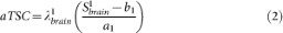
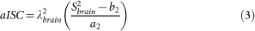
with Sibrain the signal in the brain from sequence i, λ1brain = 0.85 and λ2brain = 0.50 the correction factors for aTSC and aISC. These two factors were calculated from full density operator simulation of the sodium spin dynamics during the RF pulse sequences, with relaxation times T1 = 35 ms and T2short = 5 ms, T2long = 25 ms, based on average values in parenchyma from the literature2,20,25,45,46.
-
4
3D GM and WM and full brain (WM + GM) masks were calculated from the 1H DIR acquisitions using SPM847 in Matlab.
-
5
The aTSC and aISC maps were multiplied by the GM, WM and GM + WM masks. These masked aTSC and aISC maps can therefore be used in the following quantification section for measuring the distributions of intracellular sodium concentrations and extracellular volume fractions separately in WM and GM.


Intracellular sodium concentration (C1) and extracellular volume fraction (α) quantification
C1 and α quantification was based on a simple three-compartment model shown in Figure 2. In this model, the extracellular compartment (including interstitial volume, CSF, plasma and blood) has a constant average sodium concentration C2 = 140 mM2,20. We also considered in this study that the water (fluid) volume fraction is constant and take averages values wWM = 0.7, wGM = 0.85 and wbrain = 0.775 (mean value from WM and GM)48. We also assumed that fluid sodium signals are completely suppressed by inversion recovery in sequence 2. We will use the notation S1 = aTSC and S2 = aISC in the following equations. The value of each voxel of the map S1 is by definition equal to the total sodium concentration within each voxel, that is S1 = (C1V1 + C2V2)/Vt (Vt = total volume of the voxel). The value of each voxel of the map S2 is by definition equal to the intracellular sodium concentration only within each voxel, that is S2 = (C1V1)/Vt. From these assumptions and equations, we can calculate the unknown parameters C1 and α of interest, using the relationships given in Figure 2:


with w taking the values wWM, wGM and wbrain depending on the masked aTSC and aISC maps used. This calculation is performed for each voxel. All voxels are then recombined in 3D maps of C1 and α in WM, GM and full brain, as shown in Figure 3.
Error Propagation
Uncertainties on C1 and α for typical and extreme variations (measured as standard deviations) of S1 (aTSC), S2 (aISC), C2 (extracellular/CSF sodium concentration) and w (water fraction) can be calculated using the standard variance (or error) propagation method30. See the “Error propagation” section in Supplementary Information for more details. Typical mean values of C2, the extracellular sodium concentration (and CSF), are generally taken around 140 mM (range 135–150 mM)2,20,45,49,50, variations (std) were therefore estimated at 5 mM (typical) and 10 mM (extreme case). Typical values of water fraction w in the brain are 0.7 in white matter (WM) and 0.8–0.85 in grey matter (GM)36,48,51, with variations of the order of 0.05 (typical) and 0.10 (extreme case). The effect of these variations/uncertainties on C1 and α are shown in Table 2, for mean and std of S1 and S2 measured over full brain over 5 volunteers. In the two first std columns, all standard deviations of S1, S2, C2 and w (typical values in column 2 and extreme values in column 3) are taken into account. The last 6 std columns (columns 4–9 of the table) show the effect of individual (typical and extreme) variations from S1, S2, C2 and w. See the caption of Table 2 for more details.
Simulations
Two artificial inclusions were also added to the aTSC and aISC maps of one volunteer prior to C1 and α quantification processing, for assessing the efficiency of the method in detecting fluid-type (such as fluid cysts or other effusions, with sodium concentrations around 100–140 mM) and solid-type (such as tumors or dying cells) inclusions in the brain. The ‘fluid’ inclusion is expected to be characteristic of increase of extracellular volume fraction and probably loss of cells (and therefore loss of intracellular sodium). The ‘solid’ inclusion should be linked to increase of intracellular sodium concentration with constant extracellular volume fraction. Both inclusions were added in the brain as 10 × 10 × 10 voxels inclusions (see Supplementary Figures S1 and S3). These inclusions represent about 1.15% of the total brain volume (1000 voxels over 86571 voxels in whole GM + WM). For ‘fluid’ inclusion, aTSC = 120 mM and aISC = 5 mM (due to potential residual presence of cells, noise in data and/or imperfect fluid suppression). For ‘solid’ inclusion, aTSC = 55 mM and aISC = 25 mM. Uniform noise in the range [−2,2] (in mM) was also added to the aISC and aTSC values of the inclusion for a more realistic simulation.
References
Haacke, E. M., Brown, R. W., Thompson, M. R. & Venkatesan, R. Magnetic Resonance Imaging: Physical Principles and Sequence Design. (Wiley-Liss, New York, 1999).
Madelin, G. & Regatte, R. R. Biomedical applications of sodium MRI in vivo. J Magn Reson Imaging 38, 511–529 (2013).
Boada, F. E. et al. Loss of cell ion homeostasis and cell viability in the brain: what sodium MRI can tell us. Curr Topics Dev Biol 70, 77–101 (2005).
Sykova, E. The extracellular space in the CNS: Its regulation, volume and geometry in normal and pathological neuronal function. Neuroscientist 3, 28–41 (1997).
Nicholson, C., Kamali-Zare, P. & Tao, L. Brain Extracellular Space as a Diffusion Barrier. Comp Visual Sci 14, 309–325 (2011).
Cheek, D. B. Extracellular volume: its structure and measurement and the influence of age and disease. J Pediat 58, 103–125 (1961).
Bakay, L. The extracellular space in brain tumours. I. Morphological considerations. Brain 93, 693–698 (1970).
Sykova, E. & Nicholson, C. Diffusion in brain extracellular space. Physiol Rev 88, 1277–1340 (2008).
Xie, L. et al. Sleep drives metabolite clearance from the adult brain. Science 342, 373–377 (2013).
Cameron, I. L., Smith, N. K., Pool, T. B. & Sparks, R. L. Intracellular concentration of sodium and other elements as related to mitogenesis and oncogenesis in vivo. Cancer Res 40, 1493–1500 (1980).
Nagy, I., Lustyik, G., Lukacs, G., Nagy, V. & Balazs, G. Correlation of malignancy with the intracellular Na+:K+ ratio in human thyroid tumors. Cancer Res 43, 5395–5402 (1983).
Schepkin, V. D. et al. In vivo magnetic resonance imaging of sodium and diffusion in rat glioma at 21.1 T. Magn Reson Med 67, 1159–1166 (2012).
Rose, A. M. & Valdes, R., Jr Understanding the sodium pump and its relevance to disease. Clinic Chem 40, 1674–1685 (1994).
Thulborn, K. R., Davis, D., Snyder, J., Yonas, H. & Kassam, A. Sodium MR imaging of acute and subacute stroke for assessment of tissue viability. Neuroimag Clin N Am 15, 639–653, xi–xii, (2005).
Ouwerkerk, R., Bleich, K. B., Gillen, J. S., Pomper, M. G. & Bottomley, P. A. Tissue sodium concentration in human brain tumors as measured with 23Na MR imaging. Radiology 227, 529–537 (2003).
Kline, R. P. et al. Rapid in vivo monitoring of chemotherapeutic response using weighted sodium magnetic resonance imaging. Clin Cancer Res 6, 2146–2156 (2000).
Inglese, M. et al. Brain tissue sodium concentration in multiple sclerosis: a sodium imaging study at 3 tesla. Brain 133, 847–857 (2010).
Mellon, E. A. et al. Sodium MR imaging detection of mild Alzheimer disease: preliminary study. Am J Neuroradiol 30, 978–984 (2009).
Lu, A., Atkinson, I. & Thulborn, K. Sodium magnetic resonance imaging and its bioscale of tissue sodium concentration. Encyclopedia of Magnetic Resonance. [Harris, R. K. & Wasylishen, R. E. (ed)]. (Wiley, Chichester, 2010).
Ouwerkerk, R. Sodium MRI. Methods Mol Biol 711, 175–201 (2011).
Fleysher, L. et al. Noninvasive quantification of intracellular sodium in human brain using ultrahigh-field MRI. NMR Biomed 26, 9–19 (2013).
Reddy, R., Shinnar, M., Wang, Z. & Leigh, J. S. Multiple-quantum filters of spin-3/2 with pulses of arbitrary flip angle. J Magn Reson B 104, 148–152 (1994).
Fleysher, L., Oesingmann, N. & Inglese, M. B(0) inhomogeneity-insensitive triple-quantum-filtered sodium imaging using a 12-step phase-cycling scheme. NMR Biomed 23, 1191–1198 (2010).
Madelin, G., Lee, J. S., Inati, S., Jerschow, A. & Regatte, R. R. Sodium inversion recovery MRI of the knee joint in vivo at 7T. J Magn Reson 207, 42–52 (2010).
Stobbe, R. & Beaulieu, C. In vivo sodium magnetic resonance imaging of the human brain using soft inversion recovery fluid attenuation. Magn Reson Med 54, 1305–1310 (2005).
Madelin, G., Oesingmann, N. & Inglese, M. Double Inversion Recovery MRI with fat suppression at 7 tesla: initial experience. J Neuroimag 20, 87–92 (2010).
Redpath, T. W. & Smith, F. W. Technical note: use of a double inversion recovery pulse sequence to image selectively grey or white brain matter. Brit J Radiol 67, 1258–1263 (1994).
Meara, S. J. & Barker, G. J. Evolution of the longitudinal magnetization for pulse sequences using a fast spin-echo readout: application to fluid-attenuated inversion-recovery and double inversion-recovery sequences. Magn Reson Med 54, 241–245 (2005).
Lodish, H., Berk, A., Kaiser, C. A., Kriger, M., Scott, M. P., Bretsher, A., Ploegh, H. & Matsudaira, P. Molecular Cell Biology. [Ahr, K. (ed)] (Freeman, New York, 2007).
Ku, H. Notes on the use of propagation of error formulas. J Res Nat Bur Stand 70, 263–273 (1966).
Croarkin, C. & Tobias, P. NIST/Sematech e-handbook of statistical methods. NIST/SEMATECH, July. Available online: http://www.itl.nist.gov/div898/handbook (2006). (Date of access: 02/24/2014).
Le Bihan, D. Looking into the functional architecture of the brain with diffusion MRI. Nat Rev Neurosci 4, 469–480 (2003).
Assaf, Y. & Pasternak, O. Diffusion tensor imaging (DTI)-based white matter mapping in brain research: a review. J Mol Neurosci 34, 51–61 (2008).
Lustig, M., Donoho, D. L., Santos, J. M. & Pauly, J. M. Compressed sensing MRI. Sign Process Mag, IEEE 25, 72–82 (2008).
Aminghafari, M., Cheze, N. & Poggi, J. M. Multivariate denoising using wavelets and principal component analysis. Comput Stat Data An 50, 2381–2398 (2006).
Neeb, H., Ermer, V., Stocker, T. & Shah, N. J. Fast quantitative mapping of absolute water content with full brain coverage. NeuroImage 42, 1094–1109 (2008).
Busse, R. F., Hariharan, H., Vu, A. & Brittain, J. H. Fast spin echo sequences with very long echo trains: design of variable refocusing flip angle schedules and generation of clinical T2 contrast. Magn Reson Med 55, 1030–1037 (2006).
Pipe, J. G. et al. A new design and rationale for 3D orthogonally oversampled k-space trajectories. Magn Reson Med 66, 1303–1311 (2011).
Cunningham, C. H., Pauly, J. M. & Nayak, K. S. Saturated double-angle method for rapid B1+ mapping. Magn Reson Med 55, 1326–1333 (2006).
Schomberg, H. & Timmer, J. The gridding method for image reconstruction by Fourier transformation. IEEE Trans Med Imag 14, 596–607 (1995).
O'sullivan, J. A fast sinc function gridding algorithm for Fourier inversion in computer tomography. IEEE Trans Med Imag 4, 200–207 (1985).
Pipe, J. G. & Menon, P. Sampling density compensation in MRI: rationale and an iterative numerical solution. Magn Reson Med 41, 179–186 (1999).
Jerschow, A. From nuclear structure to the quadrupolar NMR interaction and high-resolution spectroscopy. Prog NMR Spectr 46, 63–78 (2005).
Lee, J. S., Regatte, R. R. & Jerschow, A. Optimal excitation of (23)Na nuclear spins in the presence of residual quadrupolar coupling and quadrupolar relaxation. J Chem Phys 131, 174501 (2009).
Bottomley, P. A. Sodium MRI in Man: Technique and Findings. Encyclop Magn Reson (2012).
Nagel, A. M. et al. The potential of relaxation-weighted sodium magnetic resonance imaging as demonstrated on brain tumors. Invest Radiol 46, 539–547 (2011).
Ashburner, J. et al. SPM8 Manual The FIL Methods Group (and honorary members). (2012). http://www.fil.ion.ucl.ac.uk/spm/doc/ (Date of access: 03/13/2014)
Go, K. G. The normal and pathological physiology of brain water. Adv Technical Stand Neurosurg 23, 47–142 (1997).
Boada, F. E. et al. Sodium MRI and the assessment of irreversible tissue damage during hyper-acute stroke. Transl Stroke Res 3, 236–245 (2012).
Yu, S. P. & Choi, D. W. Ions, cell volume and apoptosis. Proc Nat Acad Sci 97, 9360–9362 (2000).
Sabati, M. & Maudsley, A. A. Fast and high-resolution quantitative mapping of tissue water content with full brain coverage for clinically-driven studies. Magn Reson Imag 31, 1752–1759 (2013).
Acknowledgements
This work was supported by a CTSI Pilot Project Award at NYU Langone Medical Center, from the grant UL1 TR000038 from the National Center for Advancing Translational Sciences, National Institutes of Health. We also acknowledge financial support from the NIH grant #R01AR060238. The authors would like to thank Christopher Glielmi, Dominik Paul and Keiko Meyer of Siemens AG (Erlangen, Germany) for developing the DIR SPACE sequence for the 3 T scanner.
Author information
Authors and Affiliations
Contributions
G.M. and R.K. designed the experiments. G.M. performed the experiments, reconstructed and processed the data and performed the simulations. R.W and G.M. wrote and implemented the FLORET sequence in the Siemens scanner. G.M., R.K., R.W. and R.R.R interpreted the results and contributed to the final manuscript.
Ethics declarations
Competing interests
The authors declare no competing financial interests.
Electronic supplementary material
Supplementary Information
Supplementary Information
Rights and permissions
This work is licensed under a Creative Commons Attribution-NonCommercial-NoDerivs 3.0 Unported License. The images in this article are included in the article's Creative Commons license, unless indicated otherwise in the image credit; if the image is not included under the Creative Commons license, users will need to obtain permission from the license holder in order to reproduce the image. To view a copy of this license, visit http://creativecommons.org/licenses/by-nc-nd/3.0/
About this article

Cite this article
Madelin, G., Kline, R., Walvick, R. et al. A method for estimating intracellular sodium concentration and extracellular volume fraction in brain in vivo using sodium magnetic resonance imaging. Sci Rep 4, 4763 (2014). https://doi.org/10.1038/srep04763
Received:
Accepted:
Published:
DOI: https://doi.org/10.1038/srep04763
This article is cited by
-
A new approach to characterize cardiac sodium storage by combining fluorescence photometry and magnetic resonance imaging in small animal research
Scientific Reports (2024)
-
Imaging the transmembrane and transendothelial sodium gradients in gliomas
Scientific Reports (2021)
-
Multinuclear MRI to disentangle intracellular sodium concentration and extracellular volume fraction in breast cancer
Scientific Reports (2021)
-
THz Detection of Biomolecules in Aqueous Environments—Status and Perspectives for Analysis Under Physiological Conditions and Clinical use
Journal of Infrared, Millimeter, and Terahertz Waves (2021)
-
Validation of conductivity tensor imaging using giant vesicle suspensions with different ion mobilities
BioMedical Engineering OnLine (2020)
Comments
By submitting a comment you agree to abide by our Terms and Community Guidelines. If you find something abusive or that does not comply with our terms or guidelines please flag it as inappropriate.
