
Abstract
A simple yet efficient state reconstruction algorithm of linear regression estimation (LRE) is presented for quantum state tomography. In this method, quantum state reconstruction is converted into a parameter estimation problem of a linear regression model and the least-squares method is employed to estimate the unknown parameters. An asymptotic mean squared error (MSE) upper bound for all possible states to be estimated is given analytically, which depends explicitly upon the involved measurement bases. This analytical MSE upper bound can guide one to choose optimal measurement sets. The computational complexity of LRE is O(d4) where d is the dimension of the quantum state. Numerical examples show that LRE is much faster than maximum-likelihood estimation for quantum state tomography.
Introduction
One of the essential tasks in quantum technology is to verify the integrity of a quantum state1. Quantum state tomography has become a standard technology for inferring the state of a quantum system through appropriate measurements and estimation2,3,4,5,6,7,8. To reconstruct a quantum state, one may first perform measurements on a collection of identically prepared copies of a quantum system (data collection) and then infer the quantum state from these measurement outcomes using appropriate estimation algorithms (data analysis). Measurement on a quantum system generally gives a probabilistic result and an individual measurement outcome only provides limited information on the state of the system, even when an ideal measurement device is used. In principle, an infinite number of measurements are required to determine a quantum state precisely. However, practical quantum state tomography consists of only finite measurements and appropriate estimation algorithms. Hence, the choice of optimal measurement sets and the design of efficient state reconstruction algorithms are two critical issues in quantum state tomography.
Many results have been presented for choosing optimal measurement sets to increase the estimation accuracy and efficiency in quantum state tomography9,10,11. Several sound choices that can provide excellent performance for tomography are, for instance, tetrahedron measurement bases, cube measurement sets and mutually unbiased bases11. However, for most existing results, the optimality of a given measurement set is only verified through numerical results11. There are few methods that can analytically give an estimation error bound12,13,14, which is essential to evaluate the optimality of a measurement set15,16,17 and the appropriateness of an estimation method.
For estimation algorithms, several useful methods including maximum-likelihood estimation (MLE)2,18,19,20,21, Bayesian mean estimation (BME)2,22,23 and least-squares (LS) inversion24 have been proposed for quantum state reconstruction. The MLE method simply chooses the state estimate that gives the observed results with the highest probability. This method is asymptotically optimal in the sense that the estimation error can asymptotically achieve the Cramér-Rao bound. However, MLE usually involves solving a large number of nonlinear equations where their solutions are notoriously difficult to obtain and often not unique. Recently, an efficient method has been proposed for computing the maximum-likelihood quantum state from measurements with additive Gaussian noise, but this method is not general21. Compared to MLE, BME can always give a unique state estimate, since it constructs a state from an integral averaging over all possible quantum states with proper weights. The high computational complexity of this method significantly limits its application. The LS inversion method can be applied when measurable quantities exist that are linearly related to all density matrix elements of the quantum state being reconstructed24. However, the estimation result may be a nonphysical state and the mean squared error (MSE) bound of the estimate cannot be determined analytically.
Here, we present a new linear regression estimation (LRE) method for quantum state tomography that can identify optimal measurement sets and reconstruct a quantum state efficiently. We first convert the quantum state reconstruction into a parameter estimation problem of a linear regression model25. Next, we employ an LS algorithm to estimate the unknown parameters. The positivity of the reconstructed state can be guaranteed by an additional least-squares minimization problem. The total computational complexity is O(d4) where d is the dimension of the quantum state. In order to evaluate the performance of a chosen measurement set, an MSE upper bound for all possible states to be estimated is given analytically. This MSE upper bound depends explicitly upon the involved measurement bases and can guide us to choose the optimal measurement set. The efficiency of the method is demonstrated by examples on qubit systems.
Results
Linear regression model
We first convert the quantum state tomography problem into a parameter estimation problem of a linear regression model. Suppose the dimension of the Hilbert space  of the system of interest is d and
  is a complete basis set of orthonormal operators on the corresponding Liouville space, namely,
  , where † denotes the Hermitian adjoint and δij is the Kronecker function. Without loss of generality, let
  and
and  , such that the other bases are traceless. That is Tr(Ωi) = 0, for
  . The quantum state ρ to be reconstructed may be parameterized as

where Θi = Tr(ρΩi). Given a set of measurement bases  , each |Ψ〉〈Ψ|(n) can be parameterized under the bases
  as
as

where  .
.
When one performs measurements with measurement set  on a collection of identically prepared copies of a quantum system (with state ρ), the probability to obtain the result of |Ψ〉〈Ψ|(n) is

Assume that the total number of experiments is N and N/M experiments are performed on N/M identically prepared copies of a quantum system for each measurement basis |Ψ〉〈Ψ|(n). Denote the corresponding outcomes as  , which are independent and identically distributed. Let
  and
and  . According to the central limit theorem26, en converges in distribution to a normal distribution with mean 0 and variance
  . Using (3), we have the linear regression equations for
  ,
,

where ⊤ denotes the matrix transpose.
Note that  , d and Ψ(n) are all available, while en may be considered as the observation noise whose variance is asymptotically
  . Hence, the problem of quantum state tomography is converted into the estimation of the unknown vector Θ. Denote
  ,
,  ,
,  . We can transform the linear regression equations (4) into a compact form

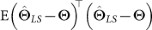
We define the MSE as  , where
  is an estimate of the quantum state ρ based on the measurement outcomes and E(·) denotes the expectation on all possible measurement outcomes. For a fixed tomography method,
  depends on the state ρ to be reconstructed and the chosen measurement bases. From a practical viewpoint, the optimality of a chosen set of measurement bases may rely upon prior information but should not depend on any specific unknown quantum state to be reconstructed. In this paper, no prior assumption is made on the state ρ to be reconstructed. Given a fixed tomography method, we use the maximum MSE for all possible states (i.e.,
  ) as the index to evaluate the performance of a chosen set of measurement bases.
Linear regression estimation
To give an estimate with high level of accuracy and low computational complexity, we employ the LS method, where the basic idea is to find an estimate  such that

where  is an estimate of Θ and W is a diagonal weighting matrix. Since the objective function is quadratic, one has the LS solution as follows:

The LS solution (7) can be calculated in a recursive way (see the Methods section). In practical experiments, the cost of time can be greatly reduced by employing a recursive reconstruction protocol since the estimate can be calculated recursively based on available data at the same time of performing measurements to acquire data.
Note that if pn = 1, we have already reconstructed the state as |Ψ〉〈Ψ|(n); if pn = 0, we should choose the following measurement basis from the orthogonal complementary space of |Ψ〉〈Ψ|(n). Hence, in general the smaller the variance of en is, the more the information can be extracted by |Ψ〉〈Ψ|(n). Therefore, the corresponding weight of the n-th regression equation should be bigger. It can be verified that if all pn are known, the LS soution  satisfying
  is asymptotically the minimum variance unbiased estimator of Θ, where V is the inverse of
  . Hence, an appropriate choice of W is the inverse of
  .
.
However, for simplicity we consider the case where W = I and the corresponding LS solution is

where  .
.
If the measurement bases  are informationally complete or overcomplete, XTX is invertible. Using (5), (8) and the statistical property of the observation noise
  (independent and asymptotically Gaussian), the estimate
  has the following properties for a fixed set of chosen measurement bases:
-
1
 is asymptotically unbiased;
 -
2
The MSE
 of
of  is asymptotically
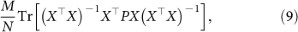
where
 .
.
 is asymptotically unbiased;
 of
of  is asymptotically
 .
.Note that pn depends upon the state to be reconstructed and the measurement basis |Ψ〉〈Ψ|(n) for  . Recall that the optimality of a chosen set of measurement bases should not depend upon any specific unknown quantum state to be reconstructed. We can take the supremum of equation (9) under all possible states to get the performance index for any given set of measurement bases
  as
as  .
.
Positivity and computational complexity
Based on the solution  obtained from (8), we can obtain a Hermitian matrix
  with
with  using (1). However,
  may have negative eigenvalues and be nonphysical due to the randomness of measurement results. In this sense,
  is called pseudo linear regression estimation (PLRE) of state ρ. A good method of pulling
  back to a physical state can reduce the MSE. In this paper, the physical estimate
  is chosen to be the closest density matrix to
  under the matrix 2-norm. In standard state reconstruction algorithms, this task is computationally intensive21. However, we can employ the fast algorithm in21 with computational complexity O(d3) to solve this problem since we have obtained a Hermitian estimate
  with
with  .
.
Since an informationally complete measurement set  requires M being O(d2), the computational complexity of (1) and XTY in (8) is O(d4). Although the computational complexity of calculating (XTX)−1 is generally O(d6), (XTX)−1 can be computed off-line before the experiment once the measurement set is determined. Hence, the total computational complexity of LRE after the data have been collected is O(d4). It is worth pointing out that for n-qubit systems,
  is diagonal for many preferred measurement sets such as tetrahedron and cube measurement sets. Fig. 1 compares the run time of our algorithm with that of a traditional MLE algorithm. Since the maximum MSE could reach 2 for the worst estimate, it is clear that our state reconstruction algorithm LRE is much more efficient than MLE with a small amount of accuracy sacrificed.

The run time and MSE of LRE and MLE for random n-qubit pure states mixed with the identity21.
The realization of MLE used the iterative method in2. The measurement bases are from the n-qubit cube measurement set and the resource is N = 39 × 4n. The simulated measurement results for every basis |Ψ〉〈Ψ|(i) are generated from a binomial distribution with probability pi = Tr(|Ψ〉〈Ψ|(i)ρ) and trials N/M. LRE is much more efficient than MLE with a small amount of accuracy sacrificed since the maximum MSE could reach 2 for the worst estimate. All timings were performed in MATLAB on the computer with 4 cores of 3 GHz Intel i5-2320 CPUs.
Optimality of measurement bases
One of the advantages of LRE is that the MSE upper bound can be given analytically as  , which is dependant explicitly upon the measurement bases. Note that if the PLRE
  is a physical state, then the MSE upper bound is asymptotically tight for the evaluation of the performance of a fixed set of measurement bases. Hence, to choose an optimal set
  , one can solve the following optimization problem:

The optimization problem can be solved in an off-line way by employing appropriate algorithms though it may be computationally intensive. We will discuss this problem in other work.
With the help of the analytical MSE upper bound, we can ascertain which one is optimal among the available measurement sets. This is demonstrated when we prove the optimality of several typical sets of measurement bases for 2-qubit systems.
For 2-qubit systems, it is convenient to chose  , where i = 4l + m; l, m = 0, 1, 2, 3; σ0 = I2×2,
  ,
,  ,
,  .
.
If the form of the measurement bases is not restricted, the minimum of the MSE upper bound  for all possible measurement bases is
  . This minimum can be reached by using the mutually unbiased measurement bases. While as in many practical experiments, if only local measurements can be performed, the minimum of the MSE upper bound
  is
is  . This minimum can be reached by using the 2-qubit cube or tetrahedron measurement set.
Fig. 2 shows the dependant relationships of the MSEs for Werner states on q (varying from 0 to 1) and different number of copies N using the cube measurement bases9. The fact that the MSE of PLRE is larger than that of LRE demonstrates that the process of pulling  back to a physical state further reduces the estimation error.

Mean squared error (MSE) for Werner states ( with
with  ) with q (varying from 0 to 1) and different numbers of copies N.
The cube measurement set is used, where the MSE upper bound is  . It can be seen that the MSE of PLRE is almost unchanged for q ∈ [0, 1] and is larger than the MSE of LRE.
Discussion
In the LRE method, data collection is achieved by performing measurements on quantum systems with given measurement bases. This process can also be accomplished by considering the evolution of quantum systems with fewer measurement bases. For example, suppose only one observable σ is given and the system evolves according to a unitary group {Ut}. At a given time t,

Suppose one measures the observable σ at time  on m identically prepared copies of a quantum system. Denote the obtained outcomes as
  and their algebraic average as
  . Note that
  are independent and identically distributed. According to the central limit theorem26,
  converges in distribution to a normal distribution with mean 0 and variance
  . We have the following linear regression equations

which are similar to (4). Hence, we can use the proposed LRE method to accomplish quantum state tomography.
The LRE method can also be extended to reconstruct quantum states with a prior information12,27,28,29 or states of open quantum systems. Actually, LRE can be applied whenever there are measurable quantities that are linearly related to all density matrix elements of the quantum system under consideration.
In conclusion, an efficient state reconstruction algorithm of linear regression estimation has been presented for quantum state tomography. The computational complexity of LRE is O(d4), which is much lower than that of MLE and BME. We have analytically provided an MSE upper bound for all possible states to be estimated, which explicitly depends upon the used measurement bases. This analytical upper bound can assist to identify optimal measurement sets. The LRE method has potential for wide applications in real experiments.
Methods
The recursive LS algorithm
For  , define
  as
as

where Wii is the i-th element of the diagonal of W and  is an estimate of Θ. Hence, the LS solution
  is equal to
  . From (7), we have

Define

Using the matrix inversion formula (see, e.g., page 19 of30)

we have

From (14), (15) and (16), the recursive form of  can be obtained as

Note that Qn is not always invertible, especially when n is small. In order to apply the recursive algorithm in this case, one may choose the initial value in (16) Q0 being a given positive matrix, while  being a given vector. From (16) and the matrix inverse formula, one has

Hence, the recursive LS algorithm can still be applied. Although the solution obtained from (17) may be slightly different from the solution obtained using (14), this does not affect the asymptotic properties of the LS solution.
The minimum of the MSE upper bound
The MSE upper bound of 2-qubit states is

Minimizing this MSE upper bound is equivalent to minimizing Tr(XTX)−1.
Denote the eigenvalues of XTX as  . Since for all possible measurement bases, we have
  ,
,  for
for  , the problem is converted into the following conditional extremum problem:

It can be proven that  reaches its minimum
  when
when  . Hence, the minimum of the MSE upper bound
  for all possible measurement bases is
  It can be verified that this minimum MSE upper bound can be reached by using the mutually unbiased measurement bases.
If only local measurements can be performed, i.e.,  ,
,  , where |Ψ〉〈Ψ|(n,1) and |Ψ〉〈Ψ|(n,2) can be parameterized as
  , k = 1, 2. And we have
  , where i = 4l + m.
Due to additional constraints  ,
,  , for k = 1, 2 and
  , the problem of minimizing the MSE upper bound can be converted into the following problem:

It can be proven that  reaches its minimum
  when
when  ,
,  . Hence, the minimum of the MSE upper bound
  is
is  . This minimum MSE upper bound can be reached by using the 2-qubit cube or tetrahedron measurement set.
References
Nielsen, M. A. & Chuang, I. L. Quantum Computation and Quantum Information (Cambridge University Press, Cambridge, England, 2001).
Paris, M. & Řeháček, J. Quantum State Estimation. Lecture Notes in Physics., Vol. 649 (Springer, Berlin, 2004).
James, D. F. V., Kwiat, P. G., Munro, W. J. & White, A. G. Measurement of qubits. Phys. Rev. A 64, 052312 (2001).
Řeháček, J., Mogilevtsev, D. & Hradil, Z. Operational tomography: fitting of data patterns. Phys. Rev. Lett. 105, 010402 (2010).
Liu, W. T., Zhang, T., Liu, J. Y., Chen, P. X. & Yuan, J. M. Experimental quantum state tomography via compressed sampling. Phys. Rev. Lett. 108, 170403 (2012).
Lundeen, J. S. & Bamber, C. Procedure for direct measurement of general quantum states using weak measurement. Phys. Rev. Lett. 108, 070402 (2012).
Salvail, J. Z. et al. characterization of polarization states of light via direct measurement. Nat. Photonics 7, 316–321 (2013).
Nunn, J., Smith, B. J., Puentes, G., Walmsley, I. A. & Lundeen, J. S. Optimal experiment design for quantum state tomography: fair, precise and minimal tomography. Phys. Rev. A 81, 042109 (2010).
Adamson, R. B. A. & Steinberg, A. M. Improving quantum state estimation with mutually unbiased bases. Phys. Rev. Lett. 105, 030406 (2010).
Wootters, W. K. & Fields, B. D. Optimal state-determination by mutually unbiased measurements. Ann. Phys. 191, 363–381 (1989).
de Burgh, M. D., Langford, N. K., Doherty, A. C. & Gilchrist, A. Choice of measurement sets in qubit tomography. Phys. Rev. A 78, 052122 (2008).
Cramer, M. et al. Efficient quantum state tomography. Nat. Commun. 1, 149 (2010).
Christandl, M. & Renner, R. Reliable quantum state tomography. Phys. Rev. Lett. 109, 120403 (2012).
Zhu, H. Quantum State Estimation and Symmetric Informationally Complete POMs (PhD thesis, National University of Singapore, Singapore, 2012).
D'Ariano, G. M. & Perinotti, P. Optimal data processing for quantum measurements. Phys. Rev. Lett. 98, 020403 (2007).
Bisio, A., Chiribella, G., D'Ariano, G. M., Facchini, S. & Perinotti, P. Optimal quantum tomography of states, measurements and transformations. Phys. Rev. Lett. 102, 010404 (2009).
Roy, A. & Scott, A. J. Weighted complex projective 2-designs from bases: optimal state determination by orthogonal measurements. J. Math. Phys. 48, 072110 (2007).
Teo, Y. S., Zhu, H., Englert, B. G., Řeháček, J. & Hradil, Z. Quantum-state reconstruction by maximizing likelihood and entropy. Phys. Rev. Lett. 107, 020404 (2011).
Teo, Y. S., Stoklasa, B., Englert, B. G., Řeháček, J. & Hradil, Z. Incomplete quantum state estimation: a comprehensive study. Phys. Rev. A 85, 042317 (2012).
Blume-Kohout, R. Hedged maximum likelihood quantum state estimation. Phys. Rev. Lett. 105, 200504 (2010).
Smolin, J. A., Gambetta, J. M. & Smith, G. Efficient method for computing the maximum-likelihood quantum state from measurements with additive Gaussian noise. Phys. Rev. Lett. 108, 070502 (2012).
Blume-Kohout, R. Optimal reliable estimation of quantum states. New J. Phys. 12, 043034 (2010).
Huszár, F. & Houlsby, N. M. T. Adaptive Bayesian quantum tomograpy. Phys. Rev. A 85, 052120 (2012).
Opatrný, T., Welsch, D.-G. & Vogel, W. Least-squares inversion for density-matrix reconstruction. Phys. Rev. A 56, 1788–1799 (1997).
Rao, C. R. & Toutenburg, H. Linear Models: Least Squares and Alternatives [2nd edn] (New York, Springer, 1999).
Chow, Y. S. & Teicher, H. Probability Theory: Independence, Interchangeability, Martingales [3rd edn] (Springer, New York, 1997).
Klimov, A. B., Björk, G. & Sánchez-Soto, L. L. Optimal quantum tomography of permutationally invariant qubits. Phys. Rev. A 87, 012109 (2013).
Gross, D., Liu, Y. K., Flammia, S. T., Becker, S. & Eisert, J. Quantum state tomography via compressed sensing. Phys. Rev. Lett. 105, 150401 (2010).
Tóth, G. et al. Permutationally invariant quantum tomography. Phys. Rev. Lett. 105, 250403 (2010).
Horn, R. A. & Johnson, C. R. Matrix Analysis (Cambridge University Press, Cambridge, 1985).
Acknowledgements
The authors would like to thank Lei Guo, Huangjun Zhu and Chuanfeng Li for helpful discussion. The work in USTC is supported by National Fundamental Research Program (Grants No. 2011CBA00200 and No. 2011CB9211200), National Natural Science Foundation of China (Grants No. 61108009 and No. 61222504), Anhui Provincial Natural Science Foundation(No. 1208085QA08). B.Q. acknowledges the support of National Natural Science Foundation of China (Grants No. 61004049, No. 61227902, No. 61374092 and No. 61134008). D.D. is supported by the Australian Research Council (DP130101658).
Author information
Authors and Affiliations
Contributions
B.Q., L.L. and D.D. developed the scheme based on linear regression model, Z.-B.H., G.-Y.X. and G.-C.G. performed the numerical simulations. All authors discussed the results and contributed to the writing of the paper. G.-Y.X. supervise the project.
Ethics declarations
Competing interests
The authors declare no competing financial interests.
Rights and permissions
This work is licensed under a Creative Commons Attribution 3.0 Unported License. To view a copy of this license, visit http://creativecommons.org/licenses/by/3.0/
About this article
Cite this article
Qi, B., Hou, Z., Li, L. et al. Quantum State Tomography via Linear Regression Estimation. Sci Rep 3, 3496 (2013). https://doi.org/10.1038/srep03496
Received:
Accepted:
Published:
DOI: https://doi.org/10.1038/srep03496
This article is cited by
-
Inapproximability of Positive Semidefinite Permanents and Quantum State Tomography
Algorithmica (2023)
-
Dimension-adaptive machine learning-based quantum state reconstruction
Quantum Machine Intelligence (2023)
-
Multi-channel quantum parameter estimation
Science China Information Sciences (2022)
-
Self-guided quantum state learning for mixed states
Quantum Information Processing (2022)
-
Local-measurement-based quantum state tomography via neural networks
npj Quantum Information (2019)
Comments
By submitting a comment you agree to abide by our Terms and Community Guidelines. If you find something abusive or that does not comply with our terms or guidelines please flag it as inappropriate.
