
Abstract
Ocean turbulent mixing is a key process in the global climate system, regulating ocean circulation and the uptake and redistribution of heat, carbon, nutrients, oxygen and other tracers. In polar oceans, turbulent heat transport additionally affects the sea ice mass balance. Due to the inaccessibility of polar regions, direct observations of turbulent mixing are sparse in the Arctic Ocean. During the year-long drift expedition “Multidisciplinary drifting Observatory for the Study of Arctic Climate” (MOSAiC) from September 2019 to September 2020, we obtained an unprecedented data set of vertical profiles of turbulent dissipation rate and water column properties, including oxygen concentration and fluorescence. Nearly 1,700 profiles, covering the upper ocean down to approximately 400 m, were collected in sets of 3 or more consecutive profiles every day, and complemented with several intensive sampling periods. This data set allows for the systematic assessment of upper ocean mixing in the Arctic, and the quantification of turbulent heat and nutrient fluxes, and can help to better constrain turbulence parameterizations in ocean circulation models.
Measurement(s) | temperature of water • conductivity of water • vertical shear • fluorescence of water • oxygen |
Technology Type(s) | temperature sensor • conductivity sensor • shear probes • flurometer • oxygen sensor |
Factor Type(s) | location and time |
Sample Characteristic - Environment | ocean |
Sample Characteristic - Location | Arctic Ocean |
Background & Summary
Sea ice cover and strong upper ocean stratification suppress vertical mixing in the Arctic Ocean, especially in the deep basins1,2. As the ice cover diminishes, momentum transfer from the atmosphere to the ocean, and the resulting turbulent mixing are expected to increase2,3,4,5. A large reservoir of heat and nutrients, originating from the Atlantic, resides at intermediate water depths. Primary production, and consequently food availability in the Arctic Ocean, is limited by nutrient supply, governed by physical transport processes6,7. Vertical mixing is hence a key process that will determine the fate of Arctic marine ecosystems8,9. In turn, increased primary production will amplify carbon dioxide fixation and drawdown. Moreover, increased heat fluxes in the ocean are an additional driver for sea ice loss, especially in winter and in regions where warm waters are located close to the surface10. Oceanic heat plays a leading role in the reduction of winter sea ice e.g. in the Barents Sea11,12 and increasingly further into the Arctic Ocean13. With longer ice-free seasons, more frequent turbulent mixing events above the continental shelf break regions might also change particle transport pathways and enhance vertical nutrient and heat transport in the Arctic14. A thorough knowledge and quantification of the Arctic Ocean mixing regime is hence crucial to understand the Arctic as a coupled system.
Direct observations of turbulent mixing in the central Arctic Ocean are still scarce, especially in the winter season. The first basin-scale survey of direct turbulence observations was conducted during the Beringia expedition in summer 2005, spanning the region from the Alaska continental shelf, crossing the North Pole to the Amundsen Basin15. Microstructure profiles were also obtained in the central Amundsen Basin e.g. in April 20071,16, and April and August 200817. Relatively more observations are available above the continental slopes north of Spitsbergen and above the Yermak Plateau (e.g. from summer 200718, during the extensive N-ICE campaign from January to June 201510, and from summer 201819), as well as from the Laptev and East Siberian Sea (e.g. in summer 200720, summer 200821, and summer 20184). In the Canada Basin, microstructure profiles have been obtained e.g. above the Chukchi slope in September 201522, and in the central basin in August 201223. Previous findings indicate that the Arctic Ocean is characterized by low levels of turbulence, compared to the other world’s oceans. Strong turbulent mixing is generally confined to the more energetic continental slope regions, either driven by tidal forces2,19 or episodic current surges14. However, previous measurements are strongly biased towards the summer season, and up to now, no data set covering a whole annual cycle of upper ocean turbulence exists.
Here, we present a comprehensive data set of vertical profiles of turbulent dissipation rates and vertically high-resolved profiles of temperature, salinity, oxygen, fluorescence and turbidity, measured with a tethered microstructure profiler in the upper ~350 m below the sea ice. Data were collected during the “Multidisciplinary drifting Observatory for the Study of Arctic Climate” (MOSAiC) drift campaign in the Arctic Ocean. The aim of this international expedition was to sample a whole annual cycle of the coupled Arctic system, using the icebreaker RV Polarstern as a drifting platform frozen into the sea ice. The experiment started in September 2019 in the Amundsen Basin, drifting northwards with the first ice floe24 parallel to the Lomonosov Ridge (legs 1 and 2, see Fig. 2a). In spring 2020, the drift speed accelerated and the floe passed the Gakkel Ridge into the Nansen Basin (leg 3). The expedition was interrupted in May/June 2020 due to the Covid-19 pandemic, when Polarstern had to leave the sampling floe to exchange personal near Svalbard. Upon return, measurements were resumed on the same floe at the northeastern flank of the Yermak Plateau (leg 4). After crossing the plateau, this first floe broke apart in Fram Strait at the end of July. Sampling continued on a second floe close to the North Pole after a short transit period back into the ice (leg 5, see Fig. 2). Except for the two sampling gaps between legs 3/4, and 4/5, profiles were obtained on a near-daily basis. Details on the course of the expedition can be found in overview publications25,26,27.
Methods
Sampling
Data acquisition
Vertical profiles were collected using tethered, free-falling microstructure probes (MSS90L, Sea & Sun Technology, Germany), through a hole drilled in the sea ice, at a minimum distance of 250 m from RV Polarstern, to avoid disturbances generated by the ship’s keel (Fig. 1). Maps of the relative position of sampling sites on the floe, with “Ocean City” being the microstructure sampling site, can be found in the overview publications25,26,27. The probe was operated with an electrical winch installed at the edge of the ice hole. Power was provided via power lines from RV Polarstern, and from generators during times when the power lines had to be disconnected to prevent damage during dynamic ice conditions. Real-time data was received and stored on an acquisition laptop connected to the winch. During legs 1 to 3 (September 2019 to May 2020), sampling was performed within a heated tent to avoid sensor damage by freezing sea water (Fig. 1b,c). After the camp was re-established on legs 4 and 5, milder temperatures allowed for sampling from an unheated pop-up tent to protect the surface electronics from precipitation (Fig. 1e). Three different probes were used throughout the drift, equipped with different auxiliary sensors to sample biogeochemical parameters (see Table 1). The probes were free-falling with an approximate sinking velocity of 0.6 m s−1. Disturbances caused by cable tension (vibrations) and ice drift were minimized by feeding sufficient slack cable.

(a) MSS winch and profiler with sensors and protection cage (ⒸLisa Grosfeld), MSS setup during (b), (c) legs 1–3 within heated tent, (d) leg 4 (prior to installation of tent, with adjacent meltpond draining into hydrohole, ⒸMorven Muilwijk) and (e) leg 5.
Microstructure measurements were complemented with time and georeference data channels using a USB 2.0 u-blox 8 Multi GNSS receiver (NAVILOCK NL-8022MU) connected to the control computer. In 59 out of 1684 profiles, GPS data were missing for various reasons (broken connection, unavailable receiver). For these profiles, starting positions were taken from the GPS receiver of the 75 kHz ADCP installed in less than 300 m distance, which sampled position data at a temporal resolution of 1 minute. For the last station, which was performed after the ADCP was recovered, ship GPS data was used.
Sampling was carried out typically every day, comprising at least 3 and often more subsequent vertical profiles to obtain reliable daily averages. The regular schedule was complemented by 7 intensive sampling periods, with repeated profiling for more than 12 hours (see Table 3). Profiles usually covered the upper ocean between 2 m below the surface to depths between 300 to 450 m, depending on drift speed and cable length. Gaps in the time series were caused by a long interruption of the drift during the exchange between legs 3 and 4 (May 17 to June 19, 2020), and during the transit north after the floe broke up in Fram Strait (July 30 to August 22, 2020).
The sampling strategy summarized above had to be adapted to logistical and environmental conditions and cross-disciplinary coordinated efforts throughout the year. Some of the key events that directly influenced our measurements are outlined below, providing additional information that helps to interpret the data set. Interruptions of a few days due to ice movement or power loss are not included here. Further information can be found in the overview publication25 and the cruise reports.
-
On November 16, 2019, high wind speeds around ~20 m s−1, resulting from a low-pressure system passing the region on November 16, caused the opening of an approximately 20 m-wide lead close to Ocean City the day after. Microstructure sampling operations were continued during the course of the wind event, providing first-hand observations of the ice-covered upper ocean under the influence of strong winds and in the proximity of a newly forming lead, e.g. a deepening of the surface mixed layer. The lead remained open for approximately one day. Throughout the course of the next days, the ice conditions changed and the previously separated parts of the floe started to converge. A massive pressure ridge started to form close by, constantly growing and moving towards Ocean City.
-
On November 24, Ocean City had to be relocated to a safer site approximately 50 m away from the initial location.
-
When regular sampling started after the drift interruption on June 27, the adjacent melt ponds had started to drain into the hydrohole used for microstructure operations. Draining had started sometime between June 22 and 25. As a consequence, the first 3–4 m of the water column consisted of a freshwater lens near freezing point (visible in Fig. 4b). The presence of this layer lead to false bottom formation at the base of the hydrohole. In the following weeks, the freshwater layer at the sampling location became successively shallower, until it could not be detected anymore in the microstructure profiles.
-
After the floe breakup and relocation northward in August, the new hydrohole was located about 300 m away from the ship in an area of 1.3 m-thick level ice. The first location chosen was about 350 m away from the ship, but due to a crack in the logistic area, Polarstern had to relocate closer to the microstructure sampling spot.
-
On August 22, 2020, the first sampling day on the second floe back north in the central Arctic Ocean, the camp had not been set up yet and profiles were performed in a pond that had melted through.
-
During the first two out of three ice stations performed during the homebound transit at the end of leg 5, microstructure measurements were performed in leads about 400 m away from the ship.
In addition to the environmental factors summarized above, the sampling was subject to several technical issues. A major problem was a low frequency (0.5 Hz) signal superimposed on most of the data channels of the profiler we initially planned to deploy (MSS075). This delayed the start of a regular sampling routine at the beginning of the expedition, and all attempts to fix this issue, including the replacement of an electronic board, were not successful. The profiler was not used, except for 15 test profiles in legs 1 and 2, which are not included in the published data set due to their questionable data quality. In addition, we encountered the following technical issues:
-
The NTC temperature sensor of the MSS046 produced a cut-off for temperatures below −0.285 °C, probably caused by a sensor output that exceeded the range of the A/D converter of the probe. On December 17, 2019, this issue was fixed by replacing the NTC sensor. However, all temperature measurements taken with the probe before that day are affected. For these first profiles (1–167) the pre-cruise manufacturer calibration was applied.
-
On January 1, 2020, the connector of the data cable of the MSS winch was repaired and fixed, after same data transmission errors during the measurements.
-
On February 5, 2020, the cable termination of the MSS winch was repaired after occasionally failures of the SDA data aquisition software.
-
On March 2, 2020, MSS046 was replaced by MSS055, to also measure biogeochemical parameters (oxygen, turbidity) before the beginning of the spring bloom (Fig. 2b).
Fig. 2 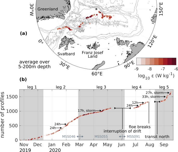
(a) Map of the Arctic Ocean, with gray lines denoting isobars with a spacing of 1000 m, and daily averaged sampling positions. Colors refer to the depth-averaged (5–200 m) dissipation rates. Bathymetric data was taken from the IBCAO data set44. (b) Time series of the cumulative number of individual profiles, with intensive sampling periods (see Table 3) and interruptions indicated. Colors refer again to the depth-averaged dissipation rates. Figure 2a was produced using the m_map matlab toolbox45.
-
On May 7, 2020, data transmission failed after 3 profiles. The issue was caused by damage of the cable connecting the winch and the deck unit, and could only fixed in the beginning of leg 4 in June. Hence, no measurements were carried out in between.
-
After the interruption of the drift, MSS055 was replaced by the new MSS091, to also measure chlorophyll fluorescence for bloom dynamics investigations.
-
On July 23, 2020, the pressure sensor of MSS091 failed. It was replaced with the pressure sensor of the malfunctioning MSS075, but another test on July 25 showed that the temperature sensor was also not working properly. The temperature sensor was replaced with the one from MSS075, and a second test profile on July 25 was performed, showing reasonable data in most data channels, except for issues with the tilt and oxygen sensors, which delivered only constant voltage output after the sensor change.
-
On August 29, 2020, the communication with the probe was interrupted and the deck unit lost power while the profiler was pulled up. Internal damage of the cable at about 100 m cable length from the termination was fixed by cutting and re-terminating the cable. The shorter cable restricted the depth range of the subsequent profiles to 250 m until the end of the expedition.
-
On September 9, 2020, the instrument was opened and cable connections were cleaned, which resolved the issue of constant voltage output for the oxygen sensor. However, this sensor gave constant readings again in later profiles, probably due to corrosion or lose electrical connections. Hence, no oxygen data is available for profiles 8202–9232, 9341, and 9346–9358, and no tilt in x-direction for profiles 8202–9358.
-
From 15 September, the communication between probe and data acquisition exhibited intermittent failures, likely due to a problem within the winch itself. Consequently, the cable was lowered manually, which was sometimes preventing the probe from free falling.

Data processing
Microstructure data are processed using a Matlab toolbox developed at the Institute for Baltic Sea Research, in collaboration with the instrument manufacturer (see section “Code Availability”). Processing routines use the Matlab Signal Processing Toolbox and the GSW Oceanographic Toolbox of TEOS-1028.
Data conversion and initial quality control
Binary raw data files are read in and converted to physical units, using the latest available manufacturer calibration (see Table 1). Data transmission errors are identified as gaps in the count sensor. The missing data lines are added and filled with NaN values. To account for the different relative position of the individual sensors on the profiler head with respect to the vertical sinking direction, the time series of all sensors are aligned with the level of the shear sensors, assuming a constant sinking velocity of 0.6 m s−1. To reduce salinity spikes, an e-folding filter is applied to the conductivity data record that adjusts the time constant of the sensor to that of the PT100 temperature sensor. In addition, visually identified sections with bad data quality in individual sensors are either linearly interpolated (e.g. spikes in conductivity) or set to NaN values (e.g. longer periods of sensor malfunction). The probes hardware includes a 1 Hz electronic high pass filter, applied directly before the sensor signal is preamplified in the sensor shaft electronics. Hence, no further high-pass or anti-aliasing filter is applied in the data processing.
The upper bound of the vertical profile is set to 2.1 m, since the low vertical velocity at the beginning of the profiles often caused a mismatch in the sensor alignment or disturbed measurements above this depth. To identify the lower bound of the profile, the maximum pressure, the vertical velocity of the probe, and the signal of acceleration sensor are used. The pressure profile is smoothed by applying a running mean (1 m vertical distance window size) and a low-pass filter (fourth order Butterworth) with a cut-off period of 1 second. The vertical sinking velocity is calculated as the time derivative (using the constant sampling frequency) of the smoothed and filtered pressure record. The lower bound of each profile is then identified as the shallowest depth within the lowermost 10% of the profile where the probe’s sinking velocity falls below 0.3 m s−1. The vertical velocity is then re-calculated by smoothing the original, cut-off record with two running means (2.3 seconds and 1 second window), and calculating the time derivative (using the constant sampling frequency).
For each shear sensor, the raw data (shraw) is converted to a voltage (V) according to
Data points in the shear records above 3 m depth (where the probe is typically not perfectly free-falling) and at low (<0.3 m s−1) sinking speeds, which indicate tension on the cable, are discarded. Vertical shear (sh) is calculated from the time derivative ∂tV as
where \({c}_{0}={\left(2\sqrt{2}\Omega {\rho }_{0}\right)}^{-1}\) is a constant including the probe-specific electronic gain of the shear sensor, Ω = 11, and the mean sea water density ρ0 = 1024 kg m−3. The derivative ∂tV is obtained using a one (left) sided gradient, calculated from two subsequent data points. This shifts the gradient profile by 0.5 ms (or 0.25 mm) relative to the other data channels. Since the higher noise of this approach is in the high frequency range of the spectrum that is not used for estimating dissipation rates (see section below), the impact on the results is small. The respective sensitivity of the individual shear sensors st is calculated dependent on the in-situ temperature T as \({s}_{t}={s}_{t}^{* }\left({c}_{0}+{c}_{1}T+{c}_{2}{T}^{2}+{c}_{3}{T}^{3}\right)\), using temperature-dependant post-cruise calibrations (see Table 2). All meta data and raw data channels are summarized in Tables 4, 5, respectively.
Dissipation rate estimates
Under the assumption of isotropic turbulence, i.e. that statistical turbulence properties are independent of direction, the rate of turbulent kinetic energy dissipation by viscous forces ε is related to the shear variance
where ν is the kinematic molecular viscosity, \(\frac{\partial u}{\partial z}\) is the vertical shear, and the overbar denotes a spatial average29. For seawater, the viscosity is temperature dependent and is approximated as \(\nu =(1.792747-0.05126103T+\)\(0.0005918645{T}^{2})\times 1{0}^{-6}\;{{\rm{m}}}^{2}\;{{\rm{s}}}^{-1}\) 30.
The shear variance is often estimated by integrating the shear spectrum over a finite wave number space. Here, we use the empirical Nasmyth spectrum31, an accepted reference shear spectrum that can be approximated in non-dimensional form32 as
where x = kLk is the (cyclic) wavenumber k, normalized by the Kolmogorov length scale \({L}_{k}={\left(\frac{{\nu }^{3}}{\varepsilon }\right)}^{0.25}\).
To calculate dissipation rates from the shear spectrum, each shear time series is subdivided into segments of 1 second, with an overlap of 0.5 seconds, and the linear trend per section is removed. A Bartlett window and a fast Fourier transformation are applied, and the one-sided power spectrum is calculated. Treating both shear sensors independently, all observed spectra within one vertical bin (here: 1 m) are averaged into a mean spectrum, that is iteratively fitted to the Nasmyth spectrum. Starting with a theoretical spectrum corresponding to a dissipation rate of ε = 10−7 W kg−1, at each iterative step the dissipation rate estimate is corrected according to the cumulative error of the fit, until this error is smaller than 0.01 or a maximum number of 50 iterative steps is reached. Working in cyclic units, the wavenumber range used for the fit is 2 cpm to the minimum of 30 cpm or 0.4 Lk. The reduction factor of 0.4 for the upper limit when using the Kolmogorov length scale is applied as the measured spectra do not follow the theoretical shape close to the edge of the inertial subrange for low turbulent dissipation rates. The final dissipation rate ε is then calculated as the mean of the two estimates from the two shear probes.
The deviation of the spectral fit, i.e. the root mean square of the deviation from the measured spectrum and the Nasmyth spectrum in the used wavenumber range, is saved as quality control parameter (see Table 6). This deviation is generally smaller (<0.1) at high dissipation rates (>10−8.5 W kg−1), and up to 0.3–0.4 at low dissipation rates.
Dissipation rate values are set to NaN if one of the following conditions is met: 1. Dissipation rate estimates for individual sensors are unrealistically low (ε < 10−13 W kg−1); 2. The covariance between shear from the individual sensors and the probe acceleration (calculated in the time domain) exceeds the threshold of 0.2; or 3. Dissipation rate estimates from the individual sensor deviate by more than a factor of 5.
Another quality control parameter included in the data set is the pseudo dissipation rate, calculated from the pseudo shear, i.e. the ratio between probe acceleration and sinking velocity, with the acceleration measured by a shear probe installed inside the pressure case of the profiler. The pseudo shear is treated identical to the physical shear, giving an estimate of pseudo dissipation rate, which is a proxy for the noise caused by the vibrations of the probe itself, and should be much smaller than the dissipation rate estimates.
Derived quantities
Based on measured in-situ temperature and conductivity, practical salinity, absolute salinity, potential and conservative Temperature, in-situ density, potential density anomaly (with sea surface as reference), the Brunt-Väisälä frequency, and the Turner angle and stability ratio were calculated using the TEOS-1028 set of equations (see Table 6). Thorpe length scales and displacements33 were calculated using the potential density profiles. Thorpe displacements are obtained relative to the statically stable, sorted density profile, using a noise level of 0.01 kg m−3.
Additional parameters included in the data set are the diffusion coefficient \({K}_{\rho }=\Gamma \frac{\varepsilon }{{N}^{2}}\), using Γ = 0.234, the buoyancy Reynolds number \(R{e}_{b}=\frac{\varepsilon }{\nu {N}^{2}}\), the Ozmidov length scale \({L}_{oz}=\sqrt{\frac{\varepsilon }{{N}^{3}}}\), and an alternative estimate of the diffusion coefficient calculated as \({K}_{\rho }=2\nu \sqrt{R{e}_{b}}\)35.
Turbidity, fluorescence and oxygen data are only processed using the manufacturer calibration and were not compared against in-situ measurements. Oxygen saturation is calculated as the ratio between the manufacturer-calibrated raw oxygen data and the partial oxygen pressure at 100% saturation \(p10{0}_{{O}_{2}}\), where \(p10{0}_{{O}_{2}}=0.2095({p}_{atm}-{p}_{{H}_{2}O})\), with patm = 1013.25 mbar being the standard air pressure at sea level and \({p}_{{H}_{2}O}=6.112{\rm{\exp }}(\frac{17.62}{(243.12+T)})\) being the saturated water vapor pressure at in-situ temperature T36. To calculate the oxygen concentration (in μmol kg−1), the oxygen saturation is multiplied with the theoretical oxygen concentration at 100% saturation derived from the in-situ temperature and density and the practical salinity37. A complete list of all derived parameters is given in Table 6.
Data Records
Data and meta data of all microstructure profiles are provided in a single netCDF file, with a vertical resolution of 1 m38. In addition, the corresponding raw data files are provided in three data sets, sorted by the individual probe used39,40,41. All data sets are published on PANGAEA (https://www.pangaea.de). The data is under a moratorium and will be publicly available as of January 1, 2023 in accordance with the MOSAiC data policy.
Technical Validation
The relative distribution of measured dissipation rates within different depth intervals is displayed in Fig. 3a. In the energetic surface layer, above 20 m depth, dissipation rates highly depend on the surface forcing, e.g. the ice drift speed, and range from 10−9 to 10−6 W kg−1. In the intermediate layer at 20–50 m depth, turbulence appears to follow the classic log-normal distribution. In deeper quiescent layers, distribution of dissipation rates accumulate near a peak at 8 × 10⁻¹⁰ (vertical dotted line in Fig. 3a), suggesting a lower detection level, i.e. noise level, for dissipation estimates of about 10−9 W kg−1.

(a) Distribution of dissipation rate in the upper 20 m (red), 20–50 m (blue) and lower than 50 m (yellow). The vertical dashed line indicates 8 × 10⁻¹⁰ W kg−1 (b) Scatter plot of the dissipation rate estimates from both shear sensors. Dashed lines indicate a deviation of ± 2.
A comparison between dissipation rate estimates from the two independent shear sensors show a generally good agreement within a factor of 2 (dashed lines in Fig. 3b), especially at dissipation rates greater than 10−8 W kg−1. At lower dissipation rates, the agreement between both sensors decreases. Overall, our quality control indicates that the presented dissipation rate estimates are robust in the presence of elevated turbulence at values greater than 10−8 W kg−1. Dissipation rate estimates at lower turbulence levels are more uncertain.
The accuracy of the auxiliary sensors given by the manufacturer are ±0.01 °C (NTC FP07); ±0.002 °C (PT100); ±0.002 mS cm−1 (conductivity). The microstructure data has not been compared with measurements from any other CTD (conductivity, temperature, depth) system that was deployed during the MOSAiC drift yet. MSS046 and MSS055 were mounted on the CTD frame and lowered together with the CTD in Ocean City (full sensor package) down to 200 m depth on January 30 (MSS046) and February 7 (MSS055). A calibration cast with a stand-alone SST 48 M CTD (serial no. 1459; Sea & Sun Technology, Germany, only pressure, temperature and salinity) attached to the MSS091 was carried out on July 29, 2020. Especially when using the auxiliary data, i.e. fluorescence, turbidity, and oxygen, we recommend to perform a cross-calibration, either using the calibration casts or several casts closest in time, to obtain quantitatively reliable data.
Usage Notes
From the presented dissipation rate measurements and vertical diffusion coefficients, turbulent fluxes of e.g. heat can be calculated. In combination with additional data sets obtained during the MOSAiC campaign, e.g. vertical profiles of nutrient concentration or the sea ice mass balance, the effect of turbulent mixing on nutrient supply and the energy balance can be assessed, providing insights into the Arctic system beyond the field of physical oceanography.
To illustrate the possibilities for scientific research this data set provides, two key quantities, the turbulent dissipation rate ε and the water column stratification N2, are displayed in Fig. 4. From September to February 2019, strong turbulent dissipation rates are confined to the near surface layer. During the course of the drift, we observed a successive deepening of the mixed layer from November to March, along with a reduction of upper ocean stratification arising from a successive increase in near surface salinity. This evolution is probably attributed to ongoing ice growth and associated brine rejection, but might partly reflect spatial gradients along the drift pathway away from the large Siberian freshwater sources. The erosion of the upper ocean stratification allowed for a deeper penetration of the surface enhanced turbulence, starting in March (Fig. 4a). In June, the presence of a fresh melt water layer appears as a strong stratification in the upper meters of the water column, and we observed an increase in upper (<75 m) ocean stratification starting mid-July. During this part of the drift, enhanced turbulent dissipation rates at greater depth are probably related to the complex topography at Yermak Plateau. After the relocation north, enhanced turbulence is again mostly confined to the upper 30 m of the water column, the surface mixed layer is considerably shallower and the upper ocean stratification is stronger compared to the first half of the drift.

Daily averaged (a) turbulent dissipation rate (W kg−1), and (b) Brunt-Väisälä frequency (s−2) in the upper 140 m. Gray isolines indicate potential density anomaly of σθ = 26, 27, 29, 30, 31 kg m−3, gray patches indicate the two major interruptions of the drift.
Code availability
The code used for data processing is available with the data set at the data repository. A publication of the processing routines on a maintained public repository is in preparation.
References
Fer, I. Weak vertical diffusion allows maintenance of cold halocline in the central Arctic. Atmospheric and Oceanic Science Letters 2, 148–152, https://doi.org/10.1080/16742834.2009.11446789 (2009).
Rippeth, T. P. et al. Tide-mediated warming of Arctic halocline by Atlantic heat fluxes over rough topography. Nature Geoscience 8, 191, https://doi.org/10.1038/ngeo2350 (2015).
Polyakov, I. V. et al. Weakening of cold halocline layer exposes sea ice to oceanic heat in the eastern Arctic Ocean. Journal of Climate 33, 8107–8123, https://doi.org/10.1175/JCLI-D-19-0976.1 (2020).
Schulz, K. et al. On the along-slope heat loss of the Boundary Current in the Eastern Arctic Ocean. Journal of Geophysical Research: Oceans 126, e2020JC016375, https://doi.org/10.1029/2020JC016375 (2021).
Rippeth, T. P. & Fine, E. C. Turbulent Mixing in a Changing Arctic Ocean. Oceanography https://doi.org/10.5670/oceanog.2022.103 (2022).
Tremblay, J.-É. et al. Global and regional drivers of nutrient supply, primary production and CO2 drawdown in the changing Arctic Ocean. Progress in Oceanography 139, 171–196, https://doi.org/10.1016/j.pocean.2015.08.009 (2015).
Schulz, K. et al. Increasing nutrient fluxes and mixing regime changes in the eastern Arctic Ocean. Geophysical Research Letters e2021GL096152, https://doi.org/10.1029/2021GL096152 (2022).
Ardyna, M. et al. Recent Arctic Ocean sea ice loss triggers novel fall phytoplankton blooms. Geophysical Research Letters 41, 6207–6212, https://doi.org/10.1002/2014GL061047 (2014).
Babin, M. Climate change tweaks Arctic marine ecosystems. Science 369, 137–138, https://doi.org/10.1126/science.abd1231 (2020).
Meyer, A., Fer, I., Sundfjord, A. & Peterson, A. K. Mixing rates and vertical heat fluxes north of Svalbard from Arctic winter to spring. Journal of Geophysical Research: Oceans 122, 4569–4586, https://doi.org/10.1002/2016JC012441 (2017).
Li, D., Zhang, R. & Knutson, T. R. On the discrepancy between observed and CMIP5 multi-model simulated Barents Sea winter sea ice decline. Nature Communications 8, 1–7, https://doi.org/10.1038/ncomms14991 (2017).
Arthun, M., Eldevik, T. & Smedsrud, L. H. The role of Atlantic heat transport in future Arctic winter sea ice loss. Journal of Climate 32, 3327–3341, https://doi.org/10.1175/JCLI-D-18-0750.1 (2019).
Polyakov, I. V. et al. Greater role for Atlantic inflows on sea-ice loss in the Eurasian Basin of the Arctic Ocean. Science 356, 285–291, https://doi.org/10.1126/science.aai8204 (2017).
Schulz, K. et al. Turbulent mixing and the formation of an intermediate nepheloid layer above the Siberian continental shelf break. Geophysical Research Letters e2021GL092988, https://doi.org/10.1029/2021GL092988 (2021).
Rainville, L. & Winsor, P. Mixing across the Arctic Ocean: Microstructure observations during the Beringia 2005 expedition. Geophysical Research Letters 35, https://doi.org/10.1029/2008GL033532 (2008).
Fer, I. Near-inertial mixing in the central Arctic Ocean. J. Phys. Oceanogr. 44, 2031–2049, https://doi.org/10.1175/JPO-D-13-0133.1 (2014).
Sirevaag, A. & Fer, I. Vertical heat transfer in the Arctic Ocean: The role of double-diffusive mixing. Journal of Geophysical Research: Oceans 117, https://doi.org/10.1029/2012JC007910 (2012).
Fer, I., Skogseth, R. & Geyer, F. Internal waves and mixing in the marginal ice zone near the Yermak Plateau. Journal of Physical Oceanography 40, 1613–1630, https://doi.org/10.1175/2010JPO4371.1 (2010).
Fer, I. et al. Tidally Forced Lee Waves Drive Turbulent Mixing Along the Arctic Ocean Margins. Geophysical Research Letters 47, e2020GL088083, https://doi.org/10.1029/2020GL088083 (2020).
Lenn, Y.-D. et al. Vertical mixing at intermediate depths in the Arctic boundary current. Geophysical Research Letters 36, https://doi.org/10.1029/2008GL036792 (2009).
Lenn, Y.-D. et al. Intermittent intense turbulent mixing under ice in the Laptev Sea continental shelf. Journal of Physical Oceanography 41, 531–547, https://doi.org/10.1175/2010JPO4425.1 (2011).
Fine, E. C., MacKinnon, J. A., Alford, M. H. & Mickett, J. B. Microstructure observations of turbulent heat fluxes in a warm-core Canada Basin eddy. Journal of Physical Oceanography 48, 2397–2418, https://doi.org/10.1175/JPO-D-18-0028.1 (2018).
Lincoln, B. J. et al. Wind-driven mixing at intermediate depths in an ice-free Arctic Ocean. Geophysical Research Letters 43, 9749–9756, https://doi.org/10.1002/2016GL070454 (2016).
Krumpen, T. et al. The MOSAiC ice floe: sediment-laden survivor from the Siberian shelf. The Cryosphere 14, 2173–2187, https://doi.org/10.5194/tc-14-2173-2020 (2020).
Rabe, B. et al. Overview of the MOSAiC expedition: Physical oceanography. Elementa: Science of the Anthropocene 10, https://doi.org/10.1525/elementa.2021.00062 (2022).
Shupe, M. D. et al. Overview of the MOSAiC expedition — Atmosphere, https://doi.org/10.1525/elementa.2021.00060 (2022).
Nicolaus, M. et al. Overview of the MOSAiC expedition: Snow and sea ice. Elem Sci Anth 10, 000046, https://doi.org/10.1525/elementa.2021.000046 (2022).
McDougall, T. J. & Barker, P. M. Getting started with TEOS-10 and the Gibbs Seawater (GSW) oceanographic toolbox. SCOR/IAPSO WG 127, 1–28 (2011).
Taylor, G. I. Statistical theory of turbulence. Proceedings of the Royal Society of London. Series A-Mathematical and Physical Sciences 151, 421–444, https://doi.org/10.1098/rspa.1935.0158 (1935).
Cisewski, B., Strass, V. H., Losch, M. & Prandke, H. Mixed layer analysis of a mesoscale eddy in the Antarctic Polar Front Zone. Journal of Geophysical Research: Oceans 113, https://doi.org/10.1029/2007JC004372 (2008).
Nasmyth, P. W. Oceanic turbulence. Ph.D. thesis, University of British Columbia. https://doi.org/10.14288/1.0302459 (1970).
Wolk, F., Yamazaki, H., Seuront, L. & Lueck, R. G. A new free-fall profiler for measuring biophysical microstructure. Journal of Atmospheric and Oceanic Technology 19, 780–793, 10.1175/1520-0426(2002)019<0780:ANFFPF>2.0.CO;2 (2002).
Thorpe, S. A. Turbulence and mixing in a Scottish Loch. Philosophical Transactions of the Royal Society of London. Series A, Mathematical and Physical Sciences 286, 125–181, https://doi.org/10.1098/rsta.1977.0112 (1977).
Osborn, T. Estimates of the local rate of vertical diffusion from dissipation measurements. Journal of Physical Oceanography 10, 83–89, 10.1175/1520-0485(1980)010<0083:EOTLRO>2.0.CO;2 (1980).
Shih, L. H., Koseff, J. R., Ivey, G. N. & Ferziger, J. H. Parameterization of turbulent fluxes and scales using homogeneous sheared stably stratified turbulence simulations. Journal of Fluid Mechanics 525, 193–214, https://doi.org/10.1017/S0022112004002587 (2005).
Garcia, H. E. & Gordon, L. I. Oxygen solubility in seawater: Better fitting equations. Limnology and oceanography 37, 1307–1312, https://doi.org/10.4319/lo.1992.37.6.1307 (1992).
Weiss, R. F. The solubility of nitrogen, oxygen and argon in water and seawater. In Deep Sea Research and Oceanographic Abstracts, vol. 17, 721–735, https://doi.org/10.1016/0011-7471(70)90037-9 (Elsevier, 1970).
Schulz, K. Turbulent microstructure profile (MSS) measurements from the MOSAiC drift, Arctic Ocean., PANGAEA, https://doi.org/10.1594/PANGAEA.939816 (2022).
Schulz, K. et al. Microstructure profiler raw data (MSS 90 L sno 046) during legs 1-3 of the MOSAiC expedition in 2019/2020., PANGAEA, https://doi.org/10.1594/PANGAEA.939820 (2022).
Schulz, K. et al. Microstructure profiler raw data (MSS55 IOW) during leg 3 of the MOSAiC expedition in 2020., PANGAEA, https://doi.org/10.1594/PANGAEA.939819 (2022).
Schulz, K. et al. Microstructure profiler raw data (MSS091) during legs 4 and 5 of the MOSAiC expedition in 2020., PANGAEA, https://doi.org/10.1594/PANGAEA.939795 (2022).
Knust, R. Polar research and supply vessel POLARSTERN operated by the Alfred-Wegener-Institute. Journal of large-scale research facilities JLSRF 3, A119–A119, https://doi.org/10.17815/jlsrf-3-163 (2017).
Nixdorf, U. et al. Mosaic extended acknowledgement. Zenodo https://doi.org/10.5281/zenodo.5541624 (2021).
Jakobsson, M. et al. The international bathymetric chart of the Arctic Ocean (IBCAO) version 3.0. Geophysical Research Letters 39, https://doi.org/10.1029/2012GL052219 (2012).
Pawlowicz, R. M_Map: A mapping package for Matlab. University of British Columbia Earth and Ocean Sciences.[Online]. Available: http://www.eos.ubc.ca/rich/map.html (2000).
Acknowledgements
Data used in this manuscript was produced as part of the international Multidisciplinary drifting Observatory for the Study of the Arctic Climate (MOSAiC) with the tag MOSAiC20192020 and the Project_ID: AWI_PS122_00. We thank all persons involved in the expedition of the Research Vessel Polarstern42 during MOSAiC in 2019–2020 as listed in the MOSAiC extended acknowledgement43, and in particular Team OCEAN and all Team Ocean friends that helped with the microstructure measurements. Financial support for the data processing was received from the German Federal Ministry for Science and Education (BMBF) and UK Natural Environment Research Council (NERC) funded PEANUTS-project (grant number 03F0804A). IF and ZK received support from the Research Council of Norway, AROMA project (294396). VM was supported by institutional funds of the Leibniz-Institut for Baltic Sea Research Warnemünde.
Funding
Open Access funding enabled and organized by Projekt DEAL.
Author information
Authors and Affiliations
Contributions
K.S. coordinated the sampling with the MSS probes during MOSAiC, processed and published the data set, wrote the initial draft, and was responsible for MSS measurements on leg 4. V.M. implemented the processing routines, coordinated the shear sensor calibration, lead on the technical trouble shooting during the expedition, and was responsible for MSS measurements during leg 2. I.F. advised on data processing and testing of the processing steps using an independent method, contributed to writing and interpretation of results. M.J. coordinates the microstructure observations at the Alfred-Wegener-Institute. M.H., J.S. and Z.K. were responsible for MSS measurements during leg 1, leg 3, and leg 5, respectively. All authors reviewed the manuscript.
Corresponding author
Ethics declarations
Competing interests
The authors declare no competing interests.
Additional information
Publisher’s note Springer Nature remains neutral with regard to jurisdictional claims in published maps and institutional affiliations.
Rights and permissions
Open Access This article is licensed under a Creative Commons Attribution 4.0 International License, which permits use, sharing, adaptation, distribution and reproduction in any medium or format, as long as you give appropriate credit to the original author(s) and the source, provide a link to the Creative Commons license, and indicate if changes were made. The images or other third party material in this article are included in the article’s Creative Commons license, unless indicated otherwise in a credit line to the material. If material is not included in the article’s Creative Commons license and your intended use is not permitted by statutory regulation or exceeds the permitted use, you will need to obtain permission directly from the copyright holder. To view a copy of this license, visit http://creativecommons.org/licenses/by/4.0/.
About this article

Cite this article
Schulz, K., Mohrholz, V., Fer, I. et al. A full year of turbulence measurements from a drift campaign in the Arctic Ocean 2019–2020. Sci Data 9, 472 (2022). https://doi.org/10.1038/s41597-022-01574-1
Received:
Accepted:
Published:
DOI: https://doi.org/10.1038/s41597-022-01574-1
This article is cited by
-
Dependency of the drag coefficient on boundary layer stability beneath drifting sea ice in the central Arctic Ocean
Scientific Reports (2024)
-
Continuous observations of the surface energy budget and meteorology over the Arctic sea ice during MOSAiC
Scientific Data (2023)
-
A dataset of direct observations of sea ice drift and waves in ice
Scientific Data (2023)
