
Abstract
Spatially explicit information on forest management at a global scale is critical for understanding the status of forests, for planning sustainable forest management and restoration, and conservation activities. Here, we produce the first reference data set and a prototype of a globally consistent forest management map with high spatial detail on the most prevalent forest management classes such as intact forests, managed forests with natural regeneration, planted forests, plantation forest (rotation up to 15 years), oil palm plantations, and agroforestry. We developed the reference dataset of 226 K unique locations through a series of expert and crowdsourcing campaigns using Geo-Wiki (https://www.geo-wiki.org/). We then combined the reference samples with time series from PROBA-V satellite imagery to create a global wall-to-wall map of forest management at a 100 m resolution for the year 2015, with forest management class accuracies ranging from 58% to 80%. The reference data set and the map present the status of forest ecosystems and can be used for investigating the value of forests for species, ecosystems and their services.
Measurement(s) | forest management type |
Technology Type(s) | Geo-Wiki toolbox |
Background & Summary
Global knowledge of forest management is critical for informing policies and decision-making on issues such as forest conservation, sustainable forest management, renewable energy, potential supply assessment of forest biomass1,2, carbon accounting3, and forest restoration practices4,5. Having a globally consistent map that characterizes the full range of forest management, from intact forests to plantations and agroforestry, could significantly facilitate these decision-making processes.
Previous work has identified some aspects of forest management in global maps, but this is usually limited to a small number of very broad classes. For example, the intact forest landscapes initiative6 provides global maps of intact forests with no signs of human activity and a minimum area of 500 km². This product, however, neglects smaller intact forests that might need attention and protection; it includes sites directly adjacent to clearcuts, which would not be considered intact by our definition; and it omits open forests in the north of Siberia and Canada. The United Nations Environment Programme World Conservation Monitoring Centre provides a natural and modified habitat layer7, which has a 1 km resolution and contains four very broad classes: likely modified (14% global forest area), potential modified (11%), potential natural (40%), and likely natural (35%). This data set, however, results from spatial overlay of anthropogenic pressure maps, each with their own uncertainty and definitions. Another quasi-global initiative is the Spatial Database of Planted Trees (SDPT V1.0)8. This is a collection of national and local scale maps from various sources, which are not always consistent in their definitions. SDPT V.1.0 recognizes 173 × 109 ha of planted forest (59% of what the Food and Agriculture Organization’s Global Forest Resources Assessment (FAO FRA) reported) and 50 × 109 ha of tree crops. Schulze et al.9 have downscaled the FAO FRA country statistics to create a global map at a 1 km resolution. The authors used 21 socio-economic and bio-physical predictor variables, but only 789 training points, collected from the literature without stratification or randomization, which limits the ability to capture spatial variability accurately.
Hence, to date, a global map of forest management covering the full range of classes has not yet been produced. Remote sensing (RS) and RS-based products have been widely used in the aforementioned studies, but, in terms of forest management, most of them identify only areas with intensive tree management (e.g., short rotation plantations, oil palm plantations10). This can be partly explained by the fact that there are insufficient reference data available, and the time series from RS are too short to cover typical forest management rotation cycles.
Here, we present the first global reference data set of forest management and a first prototype of a global forest management map derived from RS. Forests and forestry are very diverse globally, so we generalized the forest management practices that occur across countries into a set of consistent definitions, including (i) intact forests; (ii) forests with signs of human impact, including logging; (iii) planted forests; (iv) plantation forests with a rotation period of up to 15 years; (v) oil palm plantations; and (vi) agroforestry. We use the term “forest management” throughout the paper but note that our classification also contains other land-use classes with trees, such as agroforestry and oil palm plantations.
To build the reference data set, we invited experts from different parts of the world. Together, we designed and implemented a platform with an appropriate interface (see https://www.geo-wiki.org/) for crowdsourcing campaigns in which the forest experts and Geo-Wiki participants labelled time series of very high-resolution imagery to collect reference data at 226,322 locations globally. Using these data, we developed a wall-to-wall global forest management map at a 100 m resolution (PROBA-V geometry) for the year 2015. To minimize the amount of resources needed for mapping, we used the already existing classification workflow that produced the Copernicus Land Cover product for 201511. Figure 1 presents the study design.

Study design.
The reference data set is of sufficient quantity and quality to be used at regional and local scales for carrying out various forest related research. The forest management map is a prototype of generalised forest management classes and could be used in various applications, either at global, continental, or large regional scales.
Methods
Reference data collection
In February 2019, we involved forest experts from different regions around the world and organized a workshop to (1) discuss the variety of forest management practices that take place in various parts of the world; (2) explore what types of forest management information could be collected by visual interpretation of very high-resolution images from Google Maps and Microsoft Bing Maps, in combination with Sentinel time series and Normalized Difference Vegetation Index (NDVI) profiles derived from Google Earth Engine (GEE); (3) generalize and harmonize the definitions at global scale; (4) finalize the Geo-Wiki interface for the crowdsourcing campaigns; and (5) build a data set of control points (or the expert data set), which we used later to monitor the quality of the crowdsourced contributions by the participants. Based on the results of this analysis, we launched the crowdsourcing campaigns by involving a broader group of participants, which included people recruited from remote sensing, geography and forest research institutes and universities. After the crowdsourcing campaigns, we collected additional data with the help of experts. Hence, the final reference data consists of two parts: (1) a randomly stratified sample collected by crowdsourcing (49,982 locations); (2) a targeted sample collected by experts (176,340 locations, at those locations where the information collected from the crowdsourcing campaign was not large enough to ensure a robust classification).
Definitions
Table 1 contains the initial classification used for visual interpretation of the reference samples and the aggregated classes presented in the final reference data set. For the Geo-Wiki campaigns, we attempted to collect information (1) related to forest management practices and (2) recognizable from very high-resolution satellite imagery or time series of vegetation indices. The final reference data set and the final map contain an aggregation of classes, i.e., only those that were reliably distinguishable from visual interpretation of satellite imagery.
Sampling design for the crowdsourcing campaigns
Initially, we generated a random stratified sample of 110,000 sites globally. The total number of sample sites was chosen based on experiences from past Geo-Wiki campaigns12, a practical estimation of the potential number of volunteer participants that we could engage in the campaign, and the expected spatial variation in forest management. We used two spatial data sets for the stratification of the sample: World Wildlife Fund (WWF) Terrestrial Ecoregions13 and Global Forest Change14. The samples were stratified into three biomes, based on WWF Terrestrial Ecoregions (Fig. 2): boreal (25 000 sample sites), temperate (35,000 sample sites) and tropical (50,000 sample sites). Within each biome, we used Hansen’s14 Global Forest Change maps to derive areas with “forest remaining forest” 2000–2015, “forest loss or gain”, and “permanent non-forest” areas.

Biomes for sampling stratification (1 – boreal, 2 – temperate, 3 – sub-tropical and tropical).
The sample size was determined from previous experiences, taking into account the expected spatial variation in forest management within each biome. Tropical forests had the largest sample size because of increasing commodity-driven deforestation15, the wide spatial extent of plantations, and slash and burn agriculture. Temperate forests had a larger sample compared to boreal forests due to their higher fragmentation. Each sample site was classified by at least three different participants, thus accounting for human error and varying expertise16,17,18. At a later stage, following a preliminary analysis of the data collected, we increased the number of sample sites to meet certain accuracy thresholds for every mapped class (aiming to exceed 75% accuracy).
The Geo‐Wiki application
Geo‐Wiki.org is an online application for crowdsourcing and expert visual interpretation of satellite imagery, e.g., to classify land cover and land use. This application has been used in several data collection campaigns over the last decade16,19,20,21,22,23. Here, we implemented a new custom branch of Geo‐Wiki (‘Human impact on Forest’), which is devoted to the collection of forest management data (Fig. 3). Various map overlays (including satellite images from Google Maps, Microsoft Bing Maps and Sentinel 2), campaign statistics and tools to aid interpretation, such as time series profiles of NDVI, were provided as part of this Geo‐Wiki branch, giving users a range of options and choices to facilitate image classification and general data collection. Google Maps and Microsoft Bing Maps include mosaics of very high-resolution satellite and aerial imagery from different time periods and multiple image providers, including the Landsat satellites operated by NASA and USGS as base imagery to commercial image providers such as Digital Globe. More information on the spatial and temporal distribution of very high-resolution satellite imagery can be found in Lesiv et al.24. This collection of images was supplied as guidance for visual interpretation16,20. Participants could analyze time series profiles of NDVI from Landsat, Sentinel 2 and MODIS images, which were derived from Google Earth Engine (GEE). More information on tools can be found in Supplementary file 1.

Screenshot of the Geo‐Wiki interface showing a very high-resolution image from Google Maps and a sample site as a 100 mx100 m blue square, which the participants classified based on the forest management classes on the right.
The blue box in Fig. 3 corresponds to 100 m × 100 m pixels aligned with the Sentinel grid in UTM projection. It is the same geometry required for the classification workflow that is used to produce the Copernicus Land Cover product for 201511.
Before starting the campaign, the participants were shown a series of slides designed to help them gain familiarity with the interface and to train them in how to visually determine and select the most appropriate type of land use and forest management classes at each given location, thereby increasing both consistency and accuracy of the labelling tasks among experts. Once completed, the participants were shown random locations (from the random stratified sample) on the Geo‐Wiki interface and were then asked to select one of the forest management classes outlined in the Definition section (see Table 1 above).
Alternatively, if there was either insufficient quality in the available imagery, or if a participant was unable to determine the forest management type, they could skip such a site (Fig. 3). If a participant skipped a sample site because it was too difficult, other participants would then receive this sample site for classification, whereas in the case of the absence of high-resolution satellite imagery, i.e., Google Maps and Microsoft Bing Maps, this sample site was then removed from the pool of available sample sites. The skipped locations were less than 1% of the total amount of locations assigned for labeling. Table 2 shows the distribution of the skipped locations by countries, based on the subset of the crowdsourced data where all the participants agreed.
Quality assurance and data aggregation of the crowdsourced data
Based on the experience gained from previous crowdsourcing campaigns12,19, we invested in the training of the participants (130 persons in total) and overall quality assurance. Specifically, we provided initial guidelines for the participants in the form of a video and a presentation that were shown before the participants could start classifying in the forest management branch (Supplementary file 1). Additionally, the participants were asked to classify 20 training samples before contributing to the campaign. For each of these training samples, they received text‐based feedback regarding how each location should be classified. Summary information about the participants who filled in the survey at the end of the campaign (i.e., gender, age, level of education, and their country of residence) is provided in the Supplementary file 2. We would like to note that 130 participants is a high number, especially taking the complexity of the task into consideration.
Furthermore, during the campaign, sample sites that were part of the “control” data set were randomly shown to the participants. The participants received text-based feedback regarding whether the classification had been made correctly or not, with additional information and guidance. By providing immediate feedback, our intention was that participants would learn from their mistakes, increasing the quality and classification accuracy over time. If the text‐based feedback was not sufficient to provide an understanding of the correct classification, the participants were able to submit a request (“Ask the expert”) for a more detailed explanation by email.
The control set was independent of the main sample, and it was created using the same random stratified sampling procedure within each biome and the stratification by Global Forest Change maps14 (see “Sample design” section). To determine the size of the control sample, we considered two aspects: (a) the maximum number of sample sites that one person could classify during the entire campaign; (b) the frequency at which control sites would appear among the task sites (defined at 15%, which is a compromise between the classification of as many unknown locations as possible and a sufficient level of quality control, based on previous experience). Our control sample consisted of 5,000 sites. Each control sample site was classified twice by two different experts. When the two experts agreed, these sample sites were added to the final control sample. Where disagreement occurred (in 25% of cases), these sample sites were checked again by the experts and revised accordingly. During the campaign, participants had the option to disagree with the classification of the control site and submit a request with their opinion and arguments. They received an additional quality score in the situation when they were correct, but the experts were not. This procedure also ensured an increase in the quality of the control data set.
To incentivize participation and high-quality classifications, we offered prizes as part of the campaign design. The ranking system for the prize competition considered both the quality of the classifications and the number of classifications provided by a participant. The quality measure was based on the control sample discussed above. The participants randomly received a control point, which was classified in advance by the experts. For every control point, a participant could receive a maximum of +30 points (fully correct classification) to a minimum of −30 points (incorrect classification). In the case where the answer was partly correct (e.g., the participant correctly classified that the forest is managed, but misclassified the regeneration type), they received points ranging from 5 to 25.
The relative quality score for each participant was then calculated as the total sum of gained points divided by the maximum sum of points that this participant could have earned. For any subsequent data analysis, we excluded classifications from those participants whose relative quality score was less than 70%. This threshold corresponds to an average score of 10 points at each location (out of a maximum of 30 points), i.e., where participants were good at defining the aggregated forest management type but may have been less good at providing the more detailed classification.
Unfortunately, we observed some imbalance in the proportion of participants coming from different countries, e.g. there were not so many participants from the tropics. This could have resulted in interpretation errors, even when all the participants agreed on a classification. To address this, we did an additional quality check. We selected only those sample sites where all the participants agreed and then randomly checked 100 sample sites from each class. Table 3 summarizes the results of this check and explains the selection of the final classes presented in Table 1.
As a result of the actions outlined in Table 3, we compiled the final reference data set, which consisted of 49,982 consistent sample sites.
Additional expert data collection
We used the reference data set to produce a test map of forest management (the classification algorithm used is described in the next section). By checking visually and comparing against the control data set, we found that the map was of insufficient quality for many locations, especially in the case of heterogeneous landscapes. While several reasons for such an unsatisfactory result are possible, the experts agreed that a larger sample size would likely increase the accuracy of the final map, especially in areas of high heterogeneity and for forest management classes that only cover a small spatial extent. To increase the amount of high-quality training data and hence to improve the map, we collected additional data using a targeted approach. In practice, the map was uploaded to Geo-Wiki, and using the embedded drawing tools, the experts randomly checked locations on the map, focusing on their region of expertise and added classified polygons in locations where the forest management was misclassified. To limit model overfitting and oversampling of certain classes, the experts also added points for correctly mapped classes to keep the density of the points the same. This process involved a few iterations of collecting additional points and training the classification algorithm until the map accuracy reached 75%. In total, we collected an additional 176,340 training points. With the 49,982 consistent training points from the Geo-Wiki campaigns, this resulted in 226,322 (Fig. 4). This two-pronged approach would not have been possible without the exhaustive knowledge obtained from running the initial Geo-Wiki campaigns, including numerous questions raised by the campaign participants. Figure 4 also highlights in yellow the areas of very high sampling density, I.e., those collected by the experts. The sampling intensity of these areas is much higher in comparison with the randomly distributed crowdsourced locations, and these are mainly areas with very mixed forest classes or small patches, in most cases, including plantations.

Distribution of reference locations.
Classification algorithm
To produce the forest management map for the year 2015, we applied a workflow that was developed as part of the production of the Copernicus Global Land Services land cover at 100 m resolution (CGLS-LC100) collection 2 product11. A brief description of the workflow (Fig. 5), focusing on the implemented changes, is given below. A more thorough explanation, including detailed technical descriptions of the algorithms, the ancillary data used, and the intermediate products generated, can be found in the Algorithm Theoretical Basis Document (ATBD) of the CGLS-LC100 collection 2 product25.

Workflow overview for the generation of the Copernicus Global Land Cover Layers. Adapted from the Algorithm Theoretical Basis Document25.
The CGLS-LC100 collection 2 processing workflow can be applied to any satellite data, as it is unspecific to different sensors or resolutions. While the CGLS-LC100 Collection 2 product is based on PROBA-V sensor data, the workflow has already been tested with Sentinel 2 and Landsat data, thereby using it for regional/continental land cover (LC) mapping applications11,26. For generating the forest management layer, the main Earth Observation (EO) input was the PROBA-V UTM Analysis Ready Data (ARD) archive based on the complete PROBA-V L1C archive from 2014 to 2016. The ARD pre-processing included geometric transformation into a UTM coordinate system, which reduced distortions in high northern latitudes, as well as improved atmospheric correction, which converted the Top-of-Atmosphere reflectance to surface reflectance (Top-of-Canopy). In a further processing step, gaps in the 5-daily PROBA-V UTM multi-spectral image data with a Ground Sampling Distance (GSD) of ~0.001 degrees (~100 m) were filled using the PROBA-V UTM daily multi-spectral image data with a GSD of ~0.003 degrees (~300 m). This data fusion is based on a Kalman filtering approach, as in Sedano et al.27, but was further adapted to heterogonous surfaces25. Outputs from the EO pre-processing were temporally cleaned by using the internal quality flags of the PROBA-V UTM L3 data, a temporal cloud and outlier filter built on a Fourier transformation. This was done to produce consistent and dense 5-daily image stacks for all global land masses at 100 m resolution and a quality indicator, called the Data Density Indicator (DDI), used in the supervised learning process of the algorithm.
Since the total time series stack for the epoch 2015 (a three-year period including the reference year 2015 +/− 1 year) would be composed of too many proxies for supervised learning, the time and spectral dimension of the data stack had to be condensed. The spectral domain was condensed by using Vegetation Indices (VIs) instead of the original reflectance values. Overall, ten VIs based on the four PROBA-V reflectance bands were generated, which included: Normalized Difference Vegetation Index (NDVI); Enhanced Vegetation Index (EVI); Structure Intensive Pigment Index (SIPI); Normalized Difference Moisture Index (NDMI); Near-Infrared reflectance of vegetation (NIRv); Angle at NIR; HUE and VALUE of the Hue Saturation Value (HSV) color system transformation. The temporal domain of the time series VI stacks was then condensed by extracting metrics, which are used as general descriptors to enable distinguishing between the different LC classes. Overall, we extracted 266 temporal, descriptive, and textual metrics from the VI times series stacks. The temporal descriptors were derived through a harmonic model, fitted through the time series of each of the VIs based on a Fourier transformation28,29. In addition to the seven parameters of the harmonic model that describe the overall level and seasonality of the VI time series, 11 descriptive statistics (mean, standard deviation, minimum, maximum, sum, median, 10th percentile, 90th percentile, 10th – 90th percentile range, time step of the first minimum appearance, and time step of the first maximum appearance) and one textural metric (median variation of the center pixel to median of the neighbours) were generated for each VI. Additionally, the elevation, slope, aspect, and purity derived at 100 m from a Digital Elevation Model (DEM) were added. Overall, 270 metrics were extracted from the PROBA-V UTM 2015 epoch.
The main difference to the original CGLS-LC100 collection 2 algorithms is the use of forest management training data instead of the global LC reference data set, as well as only using the discrete classification branch of the algorithm. The dedicated regressor branch of the CGLS-LC100 collection 2 algorithm, i.e., outputting cover fraction maps for all LC classes, was not needed for generating the forest management layer.
In order to adapt the classification algorithm to sub-continental and continental patterns, the classification of the data was carried out per biome cluster, with the 73 biome clusters defined by the combination of several global ecological layers, which include the ecoregions 2017 dataset30, the Geiger-Koeppen dataset31, the global FAO eco-regions dataset32, a global tree-line layer33, the Sentinel-2 tiling grid and the PROBA-V imaging extent;30,31 this, effectively, resulted in the creation of 73 classification models, each with its non-overlapping geographic extent and its own training dataset. Next, in preparation for the classification procedure, the metrics of all training points were analyzed for outliers, as well as screened via an all-relevant feature selection approach for the best metric combinations (i.e., best band selection) for each biome cluster in order to reduce redundancy between parameters used in the classification. The best metrics are defined as those that have the highest separability compared to other metrics. For each metric, the separability is calculated by comparing the metric values of one class to the metric values of another class; more details can be found in the ATBD25. The optimized training data set, together with the quality indicator of the input data (DDI data set) as a weight factor, were used in the training of the Random Forest classifier. Moreover, a 5-fold cross-validation was used to optimize the classifier parameters for each generated model (one per biome).
Finally, the Random Forest classification was used to produce a hard classification, showing the discrete class for each pixel, as well as the predicted class probability. In the last step, the discrete classification results (now called the forest management map) are modified by the CGLS-LC100 collection 2 tree cover fraction layer29. Therefore, the tree cover fraction layer, showing the relative distribution of trees within one pixel, was used to remove areas with less than 10% tree cover fraction in the forest management layer, following the FAO definition of forest. Figure 6 shows the class probability layer that illustrates the model behavior, highlighting the areas of class confusion. This layer shows that there is high confusion between forest management classes in heterogeneous landscapes, e.g., in Europe and the Tropics while homogenous landscapes, such as Boreal forests, are mapped with high confidence. It is important to note that a low probability does not mean that the classification is wrong.

The predicted class probability by the Random Forest classification.
Data Records
We provide six data records34:
-
1)
The reference data set as a comma-separated file (.csv) with the following attributes:
-
“ID” is a unique location identifier.
-
“Latitude, Longitude” are centroid coordinates of a 100 m × 100 m pixel.
-
“Land_use_ID “is a land use (forest management) class:
-
0 – not forest;
-
11 – Naturally regenerating forest without any signs of management, including primary forests;
-
20 – Naturally regenerating forest with signs of management, e.g., logging, clear cuts etc;
-
31 – Planted forests;
-
32 –Plantation forests (rotation time up to 15 years);
-
40 – Oil palm plantations;
-
53 – Agroforestry;
-
−1 – samples marked as unsure in the control data set;
-
1 – samples with very high resolution imagery unavailable in the control data set.
-
-
“Flag” identifies a data origin: 1 – the crowdsourced locations (random stratified sample), 2 – the control data set (random stratified), 0 – the additional experts’ classifications following the opportunistic approach (non-random).
-
-
2)
The 100 m forest management map in a geoTiff format (see Fig. 7) with the classes presented (1).
Fig. 7 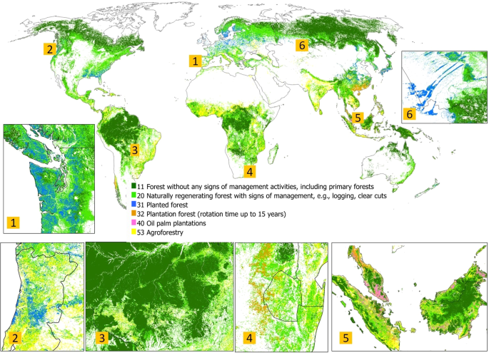
Forest management map with the following classes: 11 – Naturally regenerating forest without any signs of management, including primary forests, 20 – Naturally regenerating forest with signs of management, e.g., logging, clear cuts, 31– Planted forest; 32 – Plantation forests (rotation time up to 15 years), 40 – Oil palm plantations, 53 – Agroforestry. Six areas distributed across different continents are provided with more detailed insets: (1) planted forests in Portugal; (2) planted forests in Washington state, the USA and Vancouver Island; (3) Brazil; (4) Plantation forests in Eswatini, South Africa; (5) Peninsular Malaysia, Borneo and Sumatra; (6) planted forest in Russia and Kazakhstan.
-
3)
The predicted class probability from the Random Forest classification in a geoTiff format (see Fig. 6).
-
4)
Validation data set as a comma-separated file (.csv) with the following attributes:
-
“ID” is a unique location identifier;
-
“pixel_center_x”, “pixel_center_y” are centroid coordinates of a 100 m × 100 m pixel in lat/lon projection;
-
“first_landuse_class” is a land use class, as in (1);
-
“second_landuse_class” is a second possible land use class, as in (1), identified in case it was difficult to assign one class with high confidence.
-
-
5)
Original crowdsourced data set as a.csv table.
-
6)
Compiled FAO FRA forest statistics and mapped classes by countries into one table (.csv format).

Technical Validation
Reference data set
We have explained the quality assurance measures in detail in the section “Quality assurance and data aggregation”. In short, the data set provided is based on forest expert knowledge. We excluded all locations with high uncertainty based on expert feedback; therefore, we consider the reference data set to be of the highest quality for validation purposes.
Forest management map
We were unable to use the control data set for map validation because it does not follow a suitable sample design for rigorous statistical validation35. Therefore, we carried out an independent validation of the map by following the procedure set out in Olofsson et al.36, which allows the confidence intervals to be estimated and the area estimates to be adjusted based on the confusion matrix. We applied a random stratified sampling design to validate the map at the global level using the mapped classes as strata. We estimated that to calculate the overall accuracy of the map with a targeted accuracy of 75%, we would need approximately 2100 locations. Once we generated the sample, it was interpreted by the same set of forest experts who classified the control sample and harmonized the definitions, using Geo-Wiki. The experts were asked to identify one of the classes from Table 1. According to the guidelines35, the uncertain classifications should not be deleted. Hence, if it was difficult to determine a unique class, the experts were asked to suggest the second most likely classification at each location with uncertainty. These second classifications were used in the accuracy assessment. For example, if a validation site was classified as “planted forest” as the first classification and “naturally regenerating” as the second classification, and the mapped class was “planted forest”, then a value of 0.5 was added to the cell of the confusion matrix in the row and column “planted forest” while the other 0.5 was added to the cell in the row and column “naturally regenerating forest”.
We found the overall accuracy of the map to be 82 ± 0.01%. Table 4 provides the confusion matrix with per class accuracies. Out of 2100 locations, we had images for 2072. Hence, we consider the remaining 28 locations (~2%) as a bias of our estimates.
From the confusion matrix, it follows that planted forests (class 31) are, unsurprisingly, underestimated. This class is confused with naturally regenerated managed forests (20). The confusion matrix also indicates that there should be double the amount of planted forests than is currently shown on the map. Classes such as agroforestry, plantation forests and oil palm plantations are also underestimated due to confusion with class 20. This confusion is observed in tropical countries and could be explained by using only optical RS data, which has limited number of valid observations due to cloud coverage. Naturally regenerated forests without any signs of management (class 11) are mapped with a rather high user accuracy of 80%. This may be explained by the fact that these are quite remote homogenous areas that are easy to map from a RS point of view.
We also calculated the mapped areas of each class and the adjusted areas considering commission and omission errors as presented in Table 5. Please note that the calculations below may include biases related to the interpretation errors, which we assume are rather small.
We have calculated and compared the areas of mapped forest management classes with official FAO FRA statistics for the year 201537. Our definitions, provided in Table 1, are in line with the FAO FRA forest definitions. Specifically, naturally regenerating forests (as referred to the FAO FRA), correspond to our classes 11 and 20, planted forests (as called in the FAO FRA) correspond to the mapped classes 31 and 32. The only exception is semi-natural forests, which belong to planted forests in the FAO FRA. Moreover, we used the forest mask with a 10 percent threshold to align our map with the FRA forest definition. However, from the confusion matrix it follows that the mapped forests are overestimated. Therefore, we have also clipped the forest classes by applying 15% and 25% thresholds and then calculated areas, respectively. Table 6 provides forest areas by the FAO FRA and forest areas calculated using 3 thresholds (10%, 15% and 25%). Table 6 includes data at global level and for the 8 countries with the highest forest coverage. Statistics for all other countries could be found in the Data record38. Note that one should interpret all the areas with caution since there are discrepancies in the FAO FRA reporting by countries39.
Overall, at global scale, our estimates of forest areas are much higher than those reported in the FAO FRA. This is in line with the study by Bastin et al.40, who has demonstrated previously that there are 467 million hectares of forest in drylands that were not reported previously (e.g., see Australia in Table 6). We assume that there are also open forests (tree canopy >10% and less than 25%) in Northern latitudes that were not counted previously. For example, other RS-based research41 also recognises more forest in Russia (compared to FAO FRA national reporting) due to afforestation of abandoned arable land, expansion of forest to high latitudes and altitudes, accounting for trees in urban and cropland areas. Hence, an additional study should be undertaken to explore this finding further, especially for Russia and Canada. We show much less of the planted forests in Canada, which could be explained by the short time series used in the classification. For the Democratic Republic of the Congo and Indonesia, we show more forested areas due to the confusion between our class 20 and agroforestry. For Brazil, the mapped areas and the FAO FRA reported areas are in line.
Usage Notes
The reference data set is a unique global data set with forest management information, based on collective expert knowledge. It could be used in various biodiversity and forest related research applications, including mapping forest management at regional and local scale or the analysis of forest drivers and land use assessments.
The global forest management map is provided in spatial geoTiff format (see Data Records section) at ~100 m resolution globally. The map is spatially consistent with tree cover estimates of the Copernicus tree cover product25 with 10% threshold applied, thus facilitating comparison and overlays. Users could apply more strict thresholding if needed for their applications. We expect the global forest management map to be especially useful for broad-scale assessments of forest ecosystems, global land use modelling, biodiversity impact assessments, managed forest delineation for carbon accounting and intact forest observation.
Data from the forest management layer have already been used for the mapping of plantations in global terrestrial habitat maps42 and in the identification of global areas of biodiversity and climate mitigation importance43. However, in general, we recommend using the map for global and supra-regional applications only, rather than at the local scale, owing to the uncertainty in mapped forest management classes when examined locally, similar as to other global earth observation products44. For local usage, we would strongly recommend checking the map visually over the area of interest, or to run additional validation. Users may also consider aggregating the map to a coarser resolution.
Limitations
We would like to remind users about the non-random distribution of the targeted sample, which could be a constraint for some applications. The reference data were collated with the aim of maximizing quality and inter-user agreement rather than an equal spatial distribution.
As a result of independent validation and expert feedback, users should be aware of the following known caveats in relation to the forest management map:
-
Planted forests are underestimated, especially, in Canada and Europe.
-
Small holder oil palm plantations are mapped as agroforestry.
-
Woody and oil palm plantations are underestimated in regions with high cloud coverage and are often confused with naturally regenerated forests (class 20).
-
The map extent contains pixels with tree cover fraction of 10%, in line with the CGLS-LC100 collection 2 tree cover fraction layer but not restricted to only forest as land use. Therefore, we would recommend also applying some additional masking if possible.
It should be reiterated that this is a prototype forest management map which can be improved in the future by: (i) using longer time series of RS data and other sources of satellite data, such as Landsat and Sentinel; (ii) improving distribution and increasing in size training data set; (iii) testing other AI methodologies; and (iv) adding more thematic details. Lastly, we stress that is a global product for global applications and should not be used at sub-national level for decision making, at which scale regional maps can provide higher detail and context.
Code availability
To create the reference data set, including the control and validation data sets, we employed the Geo-Wiki application, which can be used to visually check available land cover and land use maps against very high-resolution imagery. Alternatively, users can employ the LACO-Wiki tool, which has similar functionalities and is openly available, but it requires users to upload the land cover and land use maps.
All the geographical operations were done in QGIS 3.8.0, and the accuracy matrixes were calculated in R 3.6.1., using the raster45 and dtwSat libraries46.
The forest management layer was generated using the CGLS-LC100 collection 2 processing line developed by VITO NV on behalf of the European Commission Joint Research Centre (JRC). All code was written in Python 2.7. The regional models are available as Zenodo record47, and the related biome cluster are also stored as a separate Zenodo record48.
References
Lauri, P. et al. Woody biomass energy potential in 2050. Energy Policy 66, 19–31 (2014).
Verkerk, P. J. et al. Spatial distribution of the potential forest biomass availability in Europe. Forest Ecosystems 6, 5 (2019).
Spawn, S. A., Sullivan, C. C., Lark, T. J. & Gibbs, H. K. Harmonized global maps of above and belowground biomass carbon density in the year 2010. Scientific Data 7, 112 (2020).
Löf, M., Madsen, P., Metslaid, M., Witzell, J. & Jacobs, D. F. Restoring forests: regeneration and ecosystem function for the future. New Forests 50, 139–151 (2019).
Goldstein, A. et al. Protecting irrecoverable carbon in Earth’s ecosystems. Nature Climate Change 10, 287–295 (2020).
Potapov, P. et al. The last frontiers of wilderness: Tracking loss of intact forest landscapes from 2000 to 2013. Science Advances 3, e1600821 (2017).
Gosling, J. et al. Natural and Modified Habitat Screening Layer. UN Environment Programme World Conservation Monitoring Centre (UNEP-WCMC) https://doi.org/10.34892/4q5v-gf37 (2020).
Harris, N. L., Goldman, E. D. & Gibbes, S. Spatial Database of Planted Trees Version 1.0. Technical Note. https://files.wri.org/s3fs-public/spatial-database-planted-trees.pdf (2019).
Schulze, K., Malek, Ž. & Verburg, P. H. Towards better mapping of forest management patterns: A global allocation approach. Forest Ecology and Management 432, 776–785 (2019).
Descals, A. et al. High-resolution global map of smallholder and industrial closed-canopy oil palm plantations. Earth System Science Data 13, 1211–1231 (2020).
Buchhorn, M. et al. Copernicus Global Land Cover Layers—Collection 2. Remote Sensing 12, 1044 (2020).
Lesiv, M. et al. Estimating the global distribution of field size using crowdsourcing. Global Change Biology 25, 174–186 (2019).
Olson, D. M. et al. Terrestrial Ecoregions of the World: A New Map of Life on EarthA new global map of terrestrial ecoregions provides an innovative tool for conserving biodiversity. BioScience 51, 933–938 (2001).
Hansen, M. C. et al. High-Resolution Global Maps of 21st-Century Forest Cover Change. Science 342, 850–853 (2013).
Curtis, P. G., Slay, C. M., Harris, N. L., Tyukavina, A. & Hansen, M. C. Classifying drivers of global forest loss. Science 361, 1108–1111 (2018).
See, L. et al. Harnessing the power of volunteers, the internet and Google Earth to collect and validate global spatial information using Geo-Wiki. Technological Forecasting and Social Change 98, 324–335 (2015).
Waldner, F. et al. Conflation of expert and crowd reference data to validate global binary thematic maps. Remote Sensing of Environment 221, 235–246 (2019).
Laso Bayas, J. C. et al. Validation of Automatically Generated Global and Regional Cropland Data Sets: The Case of Tanzania. Remote Sensing 9, 815 (2017).
Fritz, S. et al. Geo-Wiki: An online platform for improving global land cover. Environmental Modelling & Software 31, 110–123 (2012).
Fritz, S. et al. A global dataset of crowdsourced land cover and land use reference data. Scientific Data 4, 170075 (2017).
Schepaschenko, D. et al. Development of a global hybrid forest mask through the synergy of remote sensing, crowdsourcing and FAO statistics. Remote Sensing of Environment 162, 208–220 (2015).
Kraxner, F. et al. Mapping certified forests for sustainable management - A global tool for information improvement through participatory and collaborative mapping. Forest Policy and Economics 83, 10–18 (2017).
Schepaschenko, D. et al. Recent advances in forest observation with visual interpretation of very high-resolution imagery. Surveys in Geophysics 40, 839–862 (2019).
Lesiv, M. et al. Characterizing the Spatial and Temporal Availability of Very High Resolution Satellite Imagery in Google Earth and Microsoft Bing Maps as a Source of Reference Data. Land 7, 118 (2018).
Buchhorn, M., Bertels, L., Smets, B., Lesiv, M. & Tsendbazar, N.-E. Copernicus Global Land Service: Land Cover 100m: version 2 Globe 2015: Algorithm Theoretical Basis Document. Zenodo https://doi.org/10.5281/zenodo.3606446 (2019).
FAO. WaPOR, FAO’s Portal to Monitor Water Productivity through Open access of Remotely Sensed Derived Data. FAO https://wapor.apps.fao.org/home/WAPOR_2/1 (2019).
Sedano, F., Kempeneers, P. & Hurtt, G. A Kalman filter-based method to generate continuous time series of medium-resolution NDVI images. Remote Sensing 6, 12381–12408 (2014).
Pekel, J.-F., Cottam, A., Gorelick, N. & Belward, A. S. High-resolution mapping of global surface water and its long-term changes. Nature 540, 418–422 (2016).
Buchhorn, M. et al. Copernicus Global Land Service: Land Cover 100m: collection 2: epoch 2015: Globe. Zenodo https://doi.org/10.5281/zenodo.3243509 (2019).
Dinerstein, E. et al. An ecoregion-based approach to protecting half the terrestrial realm. BioScience 67, 534–545 (2017).
Olofsson, P. et al. A global land-cover validation data set, part I: fundamental design principles. International Journal of Remote Sensing 33, 5768–5788 (2012).
FAO. Global ecological zones for FAO forest reporting: 2010 Update. 52 http://www.fao.org/3/a-ap861e.pdf (2012).
Alaska Geobotany Center. Circumpolar Arctic Coastline and Treeline Map, http://arcticatlas.geobotany.org/catalog/entries/5421-circumpolar-arctic-coastline-and-treeline-map. (2003).
Lesiv, M. et al. Global forest management data at a 100m resolution for the year 2015. Zenodo https://doi.org/10.5281/zenodo.5879022 (2021).
Stehman, S. V. & Foody, G. M. Key issues in rigorous accuracy assessment of land cover products. Remote Sensing of Environment 231, 111199 (2019).
Olofsson, P. et al. Good practices for estimating area and assessing accuracy of land change. Remote Sensing of Environment 148, 42–57 (2014).
FAO. Global Forest Resources Assessment 2020: Main Report. FAO https://doi.org/10.4060/ca9825en (2020).
Lesiv, M. et al. Global forest management data at a 100m resolution for the year 2015 (Version 1). Zenodo https://doi.org/10.5281/zenodo.4541513 (2021).
Grainger, A. Difficulties in tracking the long-term global trend in tropical forest area. Proceedings of the National Academy of Sciences 105, 818–823 (2008).
Bastin, J.-F. et al. The extent of forest in dryland biomes. Science 356, 635–638 (2017).
Schepaschenko, D. et al. Russian forest sequesters substantially more carbon than previously reported. Sci Rep 11, 12825 (2021).
Jung, M. et al. A global map of terrestrial habitat types. Scientific Data 7, 256 (2020).
Jung, M. et al. Areas of global importance for terrestrial biodiversity, carbon, and water. bioRxiv https://doi.org/10.1101/2020.04.16.021444 (2020).
Tulbure, M. G., Hostert, P., Kuemmerle, T. & Broich, M. Regional matters: On the usefulness of regional land-cover datasets in times of global change. Remote Sensing in Ecology and Conservation. https://doi.org/10.1002/rse2.248 (2021).
Hijmans, R. J. et al. raster: Geographic Data Analysis and Modeling. https://cran.r-project.org/web/packages/raster/raster.pdf (2020).
Maus, V., Appel, M. & Giorgino, T. Time-Weighted Dynamic Time Warping for satellite image time series analysis (Software). https://cran.r-project.org/web/packages/dtwSat/index.html (2017).
Buchhorn, M. & Lesiv, M. Global forest management data at a 100m resolution for the year 2015: region-specific models. Zenodo https://doi.org/10.5281/zenodo.5849150 (2022).
Buchhorn, M. Copernicus Global Land Service: Global biome cluster layer for the 100m global land cover processing line. Zenodo https://doi.org/10.5281/zenodo.5848610 (2022).
Acknowledgements
The work was conducted by the NatureMap consortium, funded by Norway’s International Climate and Forest Initiative (NICFI). Reference data collection for the Russian Federation was supported by the Russian Science Foundation through projects No 19-77-30015 (European part of the country) and RSF-MAFF/AFFRCS No 21-46-07002 (Siberia).
Author information
Authors and Affiliations
Contributions
Myroslava Lesiv and Dmitry Schepaschenko designed the reference data collection campaigns, analysed the results and drafted the manuscript. Marcel Buchhorn ran the machine learning algorithm and produced the wall-to-wall map. Martina Dürauer designed the Geo-Wiki back- and frontend application. Linda See and Martin Jung contributed to writing and discussing the results. Ivelina Georgieva provided user support during the Geo-Wiki campaign, prepared training material. All other co-authors provided expert classifications of the reference data set and commented on the manuscript. We would like to highlight the group of experts including Dmitry Schepaschenko, Liudmila Mukhortova, Leonid Krivobokov, Elena Tikhonova, Ian Mccallum, Katharina Schulze, Andrii Bilous, Volodymyr Blyshchyk, Khongor Tsogt, Roman Vasylyshyn, Moonil Kim, Fulvio Di Fulvio, Florian Kraxner, Mikhail Yatskov, Florian Hofhansl, Carlos Luis Muñoz Brenes, Stephan Ntie, and Stephan Alexander Pietsch.
Corresponding author
Ethics declarations
Competing interests
The authors declare no competing interests.
Additional information
Publisher’s note Springer Nature remains neutral with regard to jurisdictional claims in published maps and institutional affiliations.
Supplementary information
Rights and permissions
Open Access This article is licensed under a Creative Commons Attribution 4.0 International License, which permits use, sharing, adaptation, distribution and reproduction in any medium or format, as long as you give appropriate credit to the original author(s) and the source, provide a link to the Creative Commons license, and indicate if changes were made. The images or other third party material in this article are included in the article’s Creative Commons license, unless indicated otherwise in a credit line to the material. If material is not included in the article’s Creative Commons license and your intended use is not permitted by statutory regulation or exceeds the permitted use, you will need to obtain permission directly from the copyright holder. To view a copy of this license, visit http://creativecommons.org/licenses/by/4.0/.
About this article

Cite this article
Lesiv, M., Schepaschenko, D., Buchhorn, M. et al. Global forest management data for 2015 at a 100 m resolution. Sci Data 9, 199 (2022). https://doi.org/10.1038/s41597-022-01332-3
Received:
Accepted:
Published:
DOI: https://doi.org/10.1038/s41597-022-01332-3
This article is cited by
-
Quantifying forest degradation requires a long-term, landscape-scale approach
Nature Ecology & Evolution (2024)
-
A Systematic Review of the Effects of Multi-purpose Forest Management Practices on the Breeding Success of Forest Birds
Current Forestry Reports (2024)
-
Substantial and increasing global losses of timber-producing forest due to wildfires
Nature Geoscience (2023)
-
Priority science can accelerate agroforestry as a natural climate solution
Nature Climate Change (2023)
-
Spatial database of planted forests in East Asia
Scientific Data (2023)
