
Abstract
Complex processes often arise from sequences of simpler interactions involving a few particles at a time. These interactions, however, may not be directly accessible to experiments. Here we develop the first efficient method for unravelling the causal structure of the interactions in a multipartite quantum process, under the assumption that the process has bounded information loss and induces causal dependencies whose strength is above a fixed (but otherwise arbitrary) threshold. Our method is based on a quantum algorithm whose complexity scales polynomially in the total number of input/output systems, in the dimension of the systems involved in each interaction, and in the inverse of the chosen threshold for the strength of the causal dependencies. Under additional assumptions, we also provide a second algorithm that has lower complexity and requires only local state preparation and local measurements. Our algorithms can be used to identify processes that can be characterized efficiently with the technique of quantum process tomography. Similarly, they can be used to identify useful communication channels in quantum networks, and to test the internal structure of uncharacterized quantum circuits.
Introduction
Many processes in nature arise from sequences of basic interactions, each involving a small number of physical systems. Determining the causal structure of these interactions is important both for basic science and for engineering. Often, however, the sequence of interactions giving rise to a process of interest may not be directly accessible to experiments. For example, scattering experiments in high energy physics can probe the relation between a set of incoming particles and a set of outgoing particles, but typically cannot access the individual events taking place within the scattering region. In this and similar scenarios, a fundamental problem is to characterize the causal structure of the interactions by accessing only the inputs and outputs of the process of interest, while treating the intermediate steps as a black box. We call this problem, illustrated in Fig. 1, the causal unravelling of an unknown physical process. Explicitly, the problem of causal unravelling is to determine whether an unknown process can be broken down into a sequence of simpler interactions, to determine the order of such interactions, and to determine which systems take part in each interaction. Causal unravelling can be viewed as a special case of the broader problem of causal discovery1,2, namely the task to identify the causal relations between a given set of variables. In the broad class of causal discovery problems, the distinctive features of causal unravelling are that (i) the goal is to identify a linear causal structure, corresponding to the sequence of interactions underlying the given process, and (ii) certain variables are a priori known to be ‘inputs’ (and therefore potential ‘causes’), while other variables are a priori known to be ‘outputs’ (and therefore potential ‘effects’). This scenario often arises in experimental physics, where the input/output structure is typically clear from the design of the experiment, as in the aforementioned example of scattering experiments. In principle, candidate answers can be extracted from a full tomographic characterization of the process under consideration. However, the complexity of process tomography grows exponentially in the number of inputs and outputs, making this approach unfeasible when the process involves a large number of systems.

A physical process involves a set of input systems (in the figure, A1, A2, and A3) and a set of output systems (in the figure, B1, B2, and B3). The process is the result of a sequence of interactions, each of which involves a subset of the inputs and a subset of the outputs. The problem is to infer the causal structure of the interactions solely from the input–output behaviour of the process.
In the classical domain, the problem of causal unravelling can be efficiently addressed with a variety of algorithms developed for the general problem of causal discovery1,2,3. Classical causal discovery algorithms often formulate causal relationships with graphical models and solve such models by structure learning algorithms, such as PC algorithm (named after Peter Spirtes and Clark Glymour)1, Greedy Equivalence Search4, and Max-Min Hill Climbing5. These algorithms cover a wide variety of problems, by making different sets of assumptions on the process under consideration. Typical assumptions include causal sufficiency—meaning that no variables are hidden—and causal faithfulness—meaning that the conditional independences among the variables are precisely those associated to an underlying graph used to model the causal structure. In general, however, causal discovery is intrinsically a hard problem: when no assumption is made, the complexity of all the known algorithms becomes exponential in the worst case over all possible instances6,7.
In the quantum domain, the problem of causal unravelling is made even more challenging by the presence of correlations that elude a classical explanation8,9. In recent years, the quantum extension of the notion of causal model has been addressed in a series of works10,11,12,13,14,15, providing a solid conceptual foundation to the field of quantum causal discovery. On the algorithmic side, however, the study of quantum causal models remained relatively underdeveloped. Specific instances of quantum causal discovery were studied in refs. 16,17,18, showing that quantum resources offer appealing advantages. These examples, however, were limited to simple instances, typically involving a small number of variables and/or a small number of hypotheses on the causal structure. In more general scenarios, one approach could be to perform quantum process tomography and then to infer the causal structure from the full description of the process under consideration19. As in the classical case, however, the number of queries needed by a full process tomography grows exponentially with the number of systems involved in the process, making this approach impractical as the size of the problem increases.
In this paper, we provide an efficient algorithm for unravelling the causal structure of multipartite quantum processes without resorting to full process tomography. Our algorithm is similar to the PC algorithm1 for classical causal discovery, in that it is based on a set of tests that establish the independence relations between subsets of input and output systems. We show that the algorithm has the following features:
-
1.
The number of independence tests needed to infer the causal structure scales polynomially with the number of inputs/outputs of the process. This feature is possible thanks to the special structure of the causal unravelling problem, where the goal is to establish a linear ordering of the interactions giving rise to the process under consideration.
-
2.
The independence tests produce, as a byproduct, an estimate of the strength of correlation between the various inputs and outputs of the process. In ‘Methods’, we show that this estimate can be obtained by performing a number of measurements that grows polynomially with the dimension of the systems under consideration, and that the number of measurements needed to conclude independence scales polynomially with the number of systems.
-
3.
The algorithm is exact whenever the process has bounded information loss, and satisfies a form of causal faithfulness property, namely that the strength of the causal relations, when present, is above a given threshold. When these assumptions are not satisfied, the algorithm produces an approximate result. The details of the approximate case are in Supplementary Note 6.
Moreover, the efficiency of our algorithm can be further boosted in special cases, including (i) the case where each input of a given interaction has a non-trivial causal influence on all the outputs of subsequent interactions, and (ii) the case where the process belongs to a special case of Markovian processes12,19,20,21, where each output depends only on one previous input and each input affects only one later output. We study these cases in the ‘Results’, where we devise an alternative algorithm that only requires local state preparations and local measurements. The number of queries to the process is only logarithmic in the number of input and output wires, thanks to a method that efficiently determines the correlations between input–output pairs as described in the ‘Methods’.
The remaining parts of this paper are structured as follows. In ‘Results’, we first formulate the quantum causal unravelling problem. In the second subsection, we give the main body of the efficient causal unravelling algorithm, discuss the assumptions and analyze its efficiency. The third subsection of ‘Results’ talks about the alternative algorithm designed for special cases. At the end of ‘Results’, we briefly talk about a generalization of our algorithm. Future works, interpretations and the applications of the causal unravelling algorithms are addressed in the ‘Discussion’. The ‘Methods’ section contains the detailed implementation of the independence tests used by the algorithms in ‘Results’.
Results
Problem formulation
Let us start by giving a precise formulation of the problem of quantum causal unravelling. In this problem, an experimenter is given access to a multipartite quantum process, with inputs labelled as \({A}_{1},\ldots ,{A}_{{n}_{{{{\rm{in}}}}}}\), and outputs labelled as \({B}_{1},\ldots ,{B}_{{n}_{{{{\rm{out}}}}}}\). Note that, in general, different labels may refer to the same physical system: for example, system A1 could be a single photon with a given frequency, entering in the interaction region, and system B1 could be a single photon with the same frequency, exiting the interaction region. Mathematically, the process is described by a quantum channel, that is, a completely positive trace-preserving (CPTP) linear map \({{{\mathcal{C}}}}\) transforming operators on the tensor product space \({{{{\mathcal{H}}}}}_{{A}_{1}}\otimes \cdots \otimes {{{{\mathcal{H}}}}}_{{A}_{{n}_{{{{\rm{in}}}}}}}\) to operators on the tensor product space \({{{{\mathcal{H}}}}}_{{B}_{1}}\otimes \cdots \otimes {{{{\mathcal{H}}}}}_{{B}_{{n}_{{{{\rm{out}}}}}}}\). Note that, without loss of generality, one can always assume nin = nout = n, as this condition can be satisfied by adding a number of dummy systems with one-dimensional Hilbert space. In the following, we will denote by \(L({{{\mathcal{H}}}})\) the set of linear operators on a generic Hilbert space \({{{\mathcal{H}}}}\), and by \(S({{{\mathcal{H}}}})\) the subset of density operators on \({{{\mathcal{H}}}}\), that is, the subset of operators \(\rho \in L({{{\mathcal{H}}}})\) that are positive semidefinite and have unit trace.
The problem of causal unravelling is to determine whether a multipartite process can be broken down into a sequence of interactions, as in Fig. 2, and, in the affirmative case, to determine which systems are involved in each interaction. Mathematically, the problem is to find a partition \({\{{P}_{i}\}}_{i = 1}^{m}\) of the set {A1, …, An} and a partition \({\{{Q}_{i}\}}_{i = 1}^{m}\) of the set {B1, …, Bn}, such that the multipartite process can be decomposed into a sequence of interactions, with the i-th interaction involving input systems in Pi and output systems in Qi. Such a sequential structure matches the framework of quantum combs22,23. A quantum comb is a quantum process that can be broken down into a sequence of interactions \({{{{\mathcal{C}}}}}_{1},\ldots ,{{{{\mathcal{C}}}}}_{k}\) as in Fig. 2, while each interaction \({{{{\mathcal{C}}}}}_{i}\) is a CPTP map and is called a tooth of the comb. References 22,23 give a set of necessary and sufficient conditions for determining whether a given process conforms to a quantum comb, which is equivalent to whether the process admits a causal unravelling with partitions {Pi} and {Qi}. We say a process \({{{\mathcal{C}}}}\) has a causal unravelling (P1, Q1), …, (Pm, Qm) if it can be decomposed into the form of a quantum comb with m teeth as in Fig. 2.
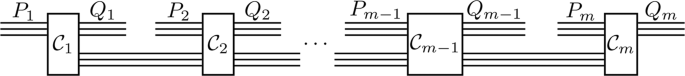
The inputs (outputs) of the processes are divided into m non-overlapping subsets. The i-th subset of the inputs (outputs) consists of the systems that enter (exit) the interaction at the i-th step (rectangular boxes in the picture). The wires connecting one interaction to the next represent intermediate systems that in this stage are not directly accessible to experiments. For example, a photon could enter the first interaction, remain as an intermediate system between the first and second interaction, and then exit the interaction region after the second interaction.
The causal unravelling of a given multipartite process determines the possible signalling relations between inputs and outputs. With respect to this decomposition, input systems at a given time can only signal to output systems at later times. The resulting pattern can be graphically illustrated by a causal graph1,2,14, as shown in Fig. 3. Note that the causal graph includes all the signalling relations that are in principle compatible with the structure of the interactions. However, a specific quantum process may not exhibit any signalling from a specific input to a specific output, even though the causal structure of the interactions would in principle permit it. When this occurs, the causal unravelling of a process may not be unique. For example, consider a bipartite process with inputs {A1, A2} and outputs {B1, B2}, with the property that A1 signals to B1 but not to B2 and A2 signals to B2 but not to B1. It is impossible to decide whether the signalling A1 → B1 happens before or after A2 → B2 since they are causally uncorrelated. Therefore, the process admits two causal unravellings: (A1, B1), (A2, B2) and (A2, B2), (A1, B1). In this case, any of the two options is a valid solution of the causal unravelling problem.
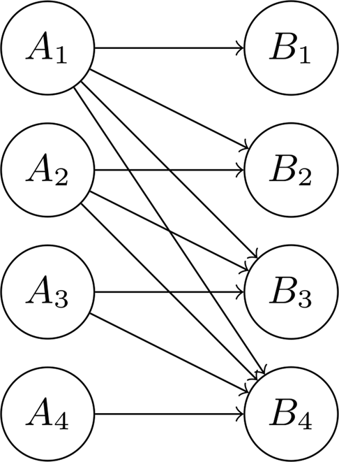
This is a bipartite graph because inputs can be independently controlled, and every two outputs are independent conditioned on all inputs.
Generally, causal discovery is a hard problem, even in the classical setting6,7. However, we will now show that, under a few assumptions, the more specific problem of quantum causal unravelling defined above can be solved efficiently. The first assumption is that the basic interactions appearing in the causal unravelling involve a small number of systems, independent of the number of inputs and outputs. At the fundamental level, this assumption is motivated by the fact that interactions are local, and typically involve a small number of systems. Mathematically, the assumption is that the cardinality of all the sets in the partitions \({\{{P}_{i}\}}_{i = 1}^{m}\) and \({\{{Q}_{i}\}}_{i = 1}^{m}\) is no larger than a constant c independent of n. For simplicity, we will first restrict our attention to the special case c = 1, meaning that the process can be broken down into interactions involving only one input and one output at a time. We will discuss larger c at the end of the ‘Results’ and in Supplementary Note 7. Hereafter, we will denote by \({\mathrm{Comb}}\)[(A1, B1), …, (An, Bn)] the set of quantum combs with n teeth where the i-th tooth has input Ai and output Bi.
In the basic c = 1 scenario illustrated above, the problem of causal unravelling is to find out which pair of systems is involved in the first interaction, which pair is involved in the second, and so on. Formally, our goal is to identify an ordering of the inputs and outputs, (Aσ(1), Bπ(1)), …, (Aσ(n), Bπ(n)) with σ and π being permutations of {1, …, n}, such that \({{{\mathcal{C}}}}\in {\mathrm{Comb}}[({A}_{\sigma (1)},{B}_{\pi (1)}),\ldots ,({A}_{\sigma (n)},{B}_{\pi (n)})]\).
To quantify the efficiency of our algorithms, we will focus on the sample complexity, namely the number of black-box queries to the channel \({{{\mathcal{C}}}}\), and on the computational complexity, including additional quantum and classical computation time measured by the number of elementary quantum gates and classical operations.
Efficient quantum causal unravelling
We now provide an efficient quantum algorithm for quantum causal unravelling. The main idea of the algorithm is to recursively find the last interaction in the decomposition of a given process. To illustrate this idea, consider the example of Fig. 3. When we remove B4, the node A4 becomes disconnected from all the other nodes, meaning that the state of system A4 does not affect the state of the other systems. By testing this independence condition, we can in principle check whether the graph of Fig. 3 is an appropriate model for the process under consideration. In general, suppose (Ax, By) are the input and output of the last interaction. Since Ax signals to only By, if we ignore By, Ax is independent of the joint system formed by all systems excluding Ax and By. This gives the following criterion that the last interaction must satisfy:
Proposition 1.22 The last interaction of a process \({{{\mathcal{C}}}}\) involves the input/output pair (Ax, By) if and only if Ax is independent of A≠xB≠y, the joint system containing all systems other than Ax and By.
More details can be found in Supplementary Note 1. By scanning the possible pairs (Ax, By), we can find if one of them satisfies the above criterion, and in the affirmative case, we can assign that pair to the last interaction. Note that, in general, there may be more than one pair that satisfy the required condition. After one pair is found, one can reduce the problem to a smaller graph containing n − 1 inputs and n − 1 outputs. If at every step a suitable pair is found, then the final result is a valid causal unravelling of the original process. If at one step no pair can be found, the algorithm will then conclude that no causal unravelling with c = 1 exists for the remaining subgraph. At this point, the algorithm can continue by considering causal unravellings with higher values of c for the remaining subgraph, which is discussed at the end of the ‘Results’ and detailed in Supplementary Note 7.
A description of the algorithm is provided in Algorithm 1. The algorithm runs in a recursive manner: for an n-tooth comb, it finds the last tooth of the comb, remove the tooth (feeds the input with an arbitrary state and discards its output), and reduces the problem to finding the causal unravelling of an (n − 1)-tooth comb. We repeat the above procedure until we reach the bottom case n = 1, and thus obtain the order of all inputs and outputs. If the last tooth cannot be found in some iteration, it means that the current channel cannot be further decomposed, and the algorithm will output the trivial causal unravelling (P, Q) where P (Q) is the set of all input (output) wires of the current channel.
Algorithm 1
Efficient quantum causal unravelling algorithm

We now discuss the efficiency of this algorithm. First, we show that the number of independence tests is polynomial in n. Let Ttest(n) be the number of independence tests required for an n-to-n channel. In this algorithm, an independence test is performed for at most each of the n2 input–output pairs (Ax, By), resulting in O(n2) independence tests. After finding a last tooth, the problem size is reduced to n − 1. Therefore, Ttest(n) can be given by the recursive relation Ttest(n) = O(n2) + Ttest(n − 1) with Ttest(1) = O(1), solving which gives Ttest(n) = O(n3).
Second, we show that the independence tests can be efficiently realized. This is a non-trivial problem, because testing whether two generic systems are in a product state is computationally hard in the worst-case scenario24. Nevertheless, in the ‘Methods’ we design a quantum circuit that performs the independence tests efficiently under assumptions of bounded information loss and causal faithfulness. Our circuit converts the independence test to the estimation of the distance between quantum states, which is done by the SWAP test25.
Now, we give the efficiency guarantee for our algorithm. We first discuss the exact case, when our algorithm produces the exact causal unravelling of \({{{\mathcal{C}}}}\) based on two assumptions. We will use a few parameters related to the Choi state26 of the process \({{{\mathcal{C}}}}\), defined as the state \(C:= ({{{\mathcal{C}}}}\otimes {{{\mathcal{I}}}})(\left|I\rangle \,\right\rangle \left\langle \,\langle I\right|)/{d}_{{{{\rm{in}}}}}\), where din is the total dimension of all the input systems, and \(\left|I\rangle \,\right\rangle =\mathop{\sum }\nolimits_{j = 1}^{{d}_{{{{\rm{in}}}}}}\left|j\right\rangle \otimes \left|j\right\rangle\) is the canonical (unnormalized) maximally entangled state. The rank of the Choi state C is called the Kraus rank of the process \({{{\mathcal{C}}}}\). Since a unitary evolution, namely a process without information loss, has Kraus rank equal to one, the Kraus rank could be interpreted as the degree of information loss introduced by the process.
An important parameter entering into the analysis is the degree of independence between systems, defined in the following. For a state ρ, we say two disjoint subsystems S and T are independent if ρST = ρS ⊗ ρT, where ρS, ρT and ρST are the marginal states of ρ on the subsystems S, T and the joint system ST, respectively. The degree of independence between S and T is then defined as \({\chi }_{1}{\left(S;T\right)}_{\rho }:= \parallel {\rho }_{ST}-{\rho }_{S}\otimes {\rho }_{T}{\parallel }_{1}\), where \(\parallel X{\parallel }_{1}:= {{\mathrm{Tr}}}\,\left[\sqrt{{X}^{{\dagger} }X}\right]\) denotes the trace norm. Clearly, \({\chi }_{1}{\left(S;T\right)}_{\rho }=0\) if and only if ρST = ρS ⊗ ρT. More generally, the trace distance is related to the probability to distinguish the states, and thus \({\chi }_{1}{\left(S;T\right)}_{\rho }\) measures the probability that an observer correctly decides whether the subsystems are independent or correlated. In the following, we will apply this definition to the Choi state C of the process \({{{\mathcal{C}}}}\). With this choice, \({\chi }_{1}{\left(S;T\right)}_{C}\) satisfies the conditions for a quantum causality measure, as defined in ref. 27.
To facilitate the efficiency analysis of our algorithm, we first put the process \({{{\mathcal{C}}}}\) in a standard form where all input and output wires have the same dimension dA. This standard form does not limit the generality of the quantum process we investigate. For a process \({{{\mathcal{C}}}}\) with input dimensions \({d}_{{A}_{1}},\ldots ,{d}_{{A}_{n}}\) and output dimensions \({d}_{{B}_{1}},\ldots ,{d}_{{B}_{n}}\), we can pick \({d}_{A}=\max \{{d}_{{A}_{1}},\ldots ,{d}_{{A}_{n}},{d}_{{B}_{1}},\ldots ,{d}_{{B}_{n}}\}\) and regard each input or output wire of \({{{\mathcal{C}}}}\) as a subspace of a dA-dimensional system, thus transforming \({{{\mathcal{C}}}}\) into a process whose wires all have dimension dA. In our analysis, we will use the Kraus rank of the process in the standard form to characterize the information loss. We assume that the information loss is bounded, which is given by the following assumption:
Assumption 1. The Kraus rank of \({{{\mathcal{C}}}}\), after transforming it into the standard form, is bounded by a polynomial of n.
To ensure that the algorithm outputs the correct causal unravelling, we further require that the process satisfies a form of causal faithfulness, meaning that the strength of causal relations is either zero or above a threshold. Using χ1 as a quantitative measure of correlation, we adopt the following assumption:
Assumption 2. There exists a number \({\chi }_{\min } > 0\) such that, for any two disjoint sets of wires S and T being tested for independence, either
-
1.
\({\chi }_{1}{\left(S;T\right)}_{C}=0\), or
-
2.
\({\chi }_{1}{\left(S;T\right)}_{C}\ge {\chi }_{\min }\),
where C is the Choi state of the quantum process \({{{\mathcal{C}}}}\).
The threshold \({\chi }_{\min }\) determines the resolution of the independence tests. To guarantee the correctness of Algorithm 1, the independence tests must be precise enough to detect correlations above this threshold with high probability. The efficiency and correctness of Algorithm 1 are given in the following theorem, whose proof is in Supplementary Note 2:
Theorem 1. Under Assumptions 1 and 2, for any confidence parameter κ0 > 0, Algorithm 1 satisfies the following conditions:
-
1.
With probability 1 − κ0, the output of Algorithm 1 is a correct causal unravelling for \({{{\mathcal{C}}}}\).
-
2.
The number of queries to \({{{\mathcal{C}}}}\) is in the order of
$${T}_{{{{\rm{sample}}}}}=O\left({n}^{3}{d}_{A}^{2}{r}_{{{{\mathcal{C}}}}}^{2}{\chi }_{\min }^{-4}\log (n{\kappa }_{0}^{-1})\right)$$(1)where \({r}_{{{{\mathcal{C}}}}}\) is the Kraus rank of \({{{\mathcal{C}}}}\) in the standard form with all wires having dimension dA.
-
3.
The computational complexity is in the order of \(O({T}_{{{{\rm{sample}}}}}n\log {d}_{A})\).
Theorem 1 guarantees that, under appropriate assumptions, the sample complexity of our algorithm is polynomial in the number of input and output systems of the process under consideration. This feature is in stark contrast with the exponential complexity of full process tomography. As a consequence, our algorithm offers a speedup over for other algorithms, such as the one proposed in ref. 19, which require process tomography as an intermediate step.
Assumptions 1 and 2 guarantee that Algorithm 1 produces an exact causal unravelling. However, both assumptions can be lifted if we only require an approximate causal unravelling, meaning that the process \({{{\mathcal{C}}}}\) is within a certain error of another process compatible with the causal unravelling output by the algorithm. In Supplementary Note 6, we formulate this approximate case and prove that the error is small under the condition that every marginal Choi state of \({{{\mathcal{C}}}}\) obtained by taking only the first k inputs and k − 1 outputs in the causal unravelling of \({{{\mathcal{C}}}}\) has polynomial rank up to a small error. This condition can be verified efficiently during the execution of Algorithm 1.
Causal unravelling with local observations
We now show that, under some assumptions on the input–output relations, one can design algorithms that have much lower sample complexity in terms of n compared to Algorithm 1, and are more experimentally friendly, in that they require only local state preparation and local measurements.
In the ‘Methods’, we show an efficient algorithm to detect the pairwise correlations between input and output wires of \({{{\mathcal{C}}}}\) with local state preparation and local measurements. The algorithm computes a Boolean matrix indij such that, with high probability, for every i and j, Ai and Bj are approximately independent whenever indij = true, and are correlated whenever indij = false. With some assumptions, this Boolean matrix indij is sufficient to give the exact causal unravelling. The first case is given by the following assumption on the process \({{{\mathcal{C}}}}\):
Assumption 3. \({{{\mathcal{C}}}}\) is a quantum comb in \({\mathrm{Comb}}\)[(Aσ(1), Bπ(1)), …, (Aσ(n), Bπ(n))], and there exists a constant \({\chi }_{\min } \,>\, 0\) such that, for any pair of input and output wires Aσ(i) and Bπ(j), if j ≥ i, then \({\chi }_{1}{\left({A}_{\sigma (i)};{B}_{\pi (j)}\right)}_{C}\ge {\chi }_{\min }\).
Assumption 3 indicates a non-trivial correlation between any pair consisting of an input system and an output system, with the property that the input system appears before the output system in the overall causal order. In other words, for any j ≥ i, \({C}_{{A}_{\sigma (i)},{B}_{\pi (j)}}\) is away from \({C}_{{A}_{\sigma (i)}}\otimes {C}_{{B}_{\pi (j)}}\) by distance \({\chi }_{\min }\). Meanwhile, Assumption 3 defines a total order of the input (output) wires, and ensures a unique causal unravelling that \({{{\mathcal{C}}}}\) is compatible with. Under this assumption, if Ai is the k-th input, namely i = σ(k), Ai is correlated with n − k + 1 output wires including every output Bπ(j) with j ≥ k, and is independent of the other outputs. In other words, if we find Ai is correlated with exactly cA(i) output wires, it must be the (n − cA(i) + 1)-th input. With this, the order of input wires can be exactly determined, and a similar statement can be applied to order the output wires.
In Supplementary Note 4, we give the details of this algorithm, and analyze its efficiency given by the following theorem:
Theorem 2. For a quantum comb \({{{\mathcal{C}}}}\in {\mathsf{Comb}}[({A}_{\sigma (1)},{B}_{\pi (1)}),\ldots ,({A}_{\sigma (n)},{B}_{\pi (n)})]\) satisfying Assumption 3, there is an algorithm that satisfies the following conditions:
-
1.
With probability 1 − κ, the algorithm outputs the correct causal unravelling (Aσ(1), Bπ(1)), …, (Aσ(n), Bπ(n)).
-
2.
The algorithm uses only local state preparations and local measurements and the number of queries to \({{{\mathcal{C}}}}\) is in the order of
$$N=O\left({d}_{A}^{6}{d}_{B}^{6}{\chi }_{\min }^{-2}\log (n{d}_{A}{d}_{B}{\kappa }^{-1})\right),$$(2)\({where}\,{d}_{A}:= \mathop{\max }\limits_{i}{d}_{{A}_{i}},{d}_{B}:= \mathop{\max }\limits_{j}{d}_{{B}_{j}}\).
-
3.
The computational complexity is in the order of \(O(Nn(n+{d}_{A}+{d}_{B}^{4}))\).
Note the sample complexity of this algorithm grows only logarithmically with n.
A similar idea could be adopted to the case where the process belongs to a special case of Markovian processes12,19,20,21, where each output depends only on one previous input and each input affects only one later output. This indicates that the process is decomposable to a tensor product of n channels each with one input and one output. In our problem, the order of inputs and outputs is unknown, and we have the following assumption:
Assumption 4. The process C is a tensor product of n channels, \({{{\mathcal{C}}}}{ = \bigotimes }_{i = 1}^{n}{{{{\mathcal{C}}}}}_{i}\) with \({{{{\mathcal{C}}}}}_{i}:{{{{\mathcal{H}}}}}_{{A}_{i}}\to {{{{\mathcal{H}}}}}_{{B}_{\pi ^{\prime} (i)}}\) for some permutation \(\pi ^{\prime}\).
Since each output is related to at most one input and each input affects at most one output, after obtaining indij, we can obtain the causal unravelling by matching each input–output pair (Ai, Bj) with indij = false.
If there exists a threshold \({\chi }_{\min } \,>\, 0\) such that either \({\chi }_{1}{\left({A}_{i};{B}_{j}\right)}_{C}=0\) or \({\chi }_{1}{\left({A}_{i};{B}_{j}\right)}_{C}\ge {\chi }_{\min }\) holds for every Ai and Bj, then the algorithm has the same complexity as in Theorem 2 that is logarithmic in n. However, in case a threshold \({\chi }_{\min }\) is not known, we can still show that the algorithm is efficient yet produces an approximate answer with an error bound defined by the diamond norm28. The diamond norm, also known as the completely bounded trace norm, is a distance measure between channels defined for \({{{\mathcal{C}}}},{{{\mathcal{D}}}}:L({{{{\mathcal{H}}}}}_{A})\to L({{{{\mathcal{H}}}}}_{B})\) as \(\parallel {{{\mathcal{C}}}}-{{{\mathcal{D}}}}{\parallel }_{\lozenge }:= \mathop{\max }\limits_{\rho \in S({{{{\mathcal{H}}}}}_{A}\otimes {{{{\mathcal{H}}}}}_{A})}\parallel ({{{\mathcal{C}}}}\otimes {{{{\mathcal{I}}}}}_{A})(\rho )-({{{\mathcal{D}}}}\otimes {{{{\mathcal{I}}}}}_{A})(\rho ){\parallel }_{1}\), where \({{{{\mathcal{I}}}}}_{A}:L({{{{\mathcal{H}}}}}_{A})\to L({{{{\mathcal{H}}}}}_{A})\) is the identity map. The diamond norm measures the maximum probability to distinguish two channels, and is tighter than the trace distance since \(\parallel {{{\mathcal{C}}}}-{{{\mathcal{D}}}}{\parallel }_{\lozenge }\le \parallel C-D{\parallel }_{1}\) for all channels \({{{\mathcal{C}}}}\) and \({{{\mathcal{D}}}}\) with Choi states C and D. The error bound is stated in the following theorem, whose proof is in Supplementary Note 5.
Theorem 3. For a quantum process \({{{\mathcal{C}}}}\) satisfying Assumption 4, there is an algorithm that outputs a causal unravelling (A1, Bπ(1)), …, (An, Bπ(n)) satisfying the following conditions:
-
1.
With probability 1 − κ, the causal unravelling is approximately correct in the following sense:
$$\exists {{{\mathcal{D}}}}\in {\mathsf{Comb}}[({A}_{1},{B}_{\pi (1)}),\ldots ,({A}_{n},{B}_{\pi (n)})],\,\parallel {{{\mathcal{C}}}}-{{{\mathcal{D}}}}{\parallel }_{\lozenge }\le \varepsilon \,.$$(3) -
2.
The algorithm uses only local state preparations and local measurements and the number of queries to \({{{\mathcal{C}}}}\) is in the order of
$$N=O\left({n}^{2}{d}_{A}^{8}{d}_{B}^{6}{\varepsilon }^{-2}\log (n{d}_{A}{d}_{B}{\kappa }^{-1})\right),$$(4)\(where\,{d}_{A}:= \mathop{\max }\limits_{i}{d}_{{A}_{i}}\) and \({d}_{B}:= \mathop{\max }\limits_{j}{d}_{{B}_{j}}\).
-
3.
The computational complexity is in the order of \(O(Nn(n+{d}_{A}+{d}_{B}^{4}))\).
Causal unravelling with interactions between more inputs and outputs
In the algorithms shown so far, we assumed that the process under consideration admits a causal unravelling where each interaction involves exactly one input and one output. More generally, Algorithm 1 can be easily extended to the scenario where each interaction involves at most c inputs and c outputs of the original process. Instead of considering each wire separately, the idea is to consider a subset of at most c input (output) wires and perform independence tests on the subsets.
In Algorithm 1, one enumerates an input–output pair (Ax, By) and checks whether it is the last tooth by performing an independence test between Ax and A≠xB≠y. To deal with larger c, we replace this procedure by enumerating a subset of input wires \(P\subset \{{A}_{1},\ldots ,{A}_{{n}_{{{{\rm{in}}}}}}\}\) and a subset of output wires \(Q\subset \{{B}_{1},\ldots ,{B}_{{n}_{{{{\rm{out}}}}}}\}\), satisfying ∣P∣ ≤ c and ∣Q∣ ≤ c. Then we check whether (P, Q) is the last tooth of \({{{\mathcal{C}}}}\), which, according to Proposition 1, is equivalent to checking the independence between P and A∉PB∉Q ≔ {Ai∣Ai ∉ P} ∪ {Bj∣Bj ∉ Q}. The independence tests can still be implemented with SWAP tests. Like Algorithm 1, after we decide (P, Q) to be the last tooth, the wires in P and Q are removed from consideration, and the problem is reduced to the causal unravelling of a smaller channel. This process is done recursively until one reaches the bottom case. We give the detailed algorithm and analysis in Supplementary Note 7. For constant c, under some assumptions, the complexity of the algorithm is still polynomial in n and dA, while the exponent depends on c.
Discussion
In this paper we developed an efficient algorithm for discovering linear causal structures between the inputs and outputs of a multipartite quantum process. Our algorithm provides a partial solution to the more general quantum causal discovery problem, whose goal is to produce a full causal graph describing arbitrary causal correlations in an arbitrary set of quantum variables. Our algorithm can be used as the first step for quantum causal discovery, and to obtain the full causal structure, additional tests may be adopted to detect signalling between more subsets of input and output wires. Since the most general quantum causal discovery problem is intrinsically hard, an interesting direction for future work is to examine to what extent the problem of quantum causal discovery can be solved by an efficient algorithm in scenarios beyond the linear structure analysed in this work.
The efficiency of our algorithms relies on some assumptions. For Algorithm 1, the low-rank assumption is the key in both the exact case (Assumption 1) and the approximate case discussed in Supplementary Note 6. This assumption avoids the computational difficulty of deciding whether a completely general state is a product state24. Physically, a quantum process has a low rank if the number of uncontrolled particles entering and/or exiting the interaction region is small. In this picture, the uncontrolled particles in the input can be regarded as sources of environmental noise, and the uncontrolled particles in the output are responsible for information loss in the process. Intuitively, without the low-rank assumption, the causal correlations will be obscured by the noise, and it will be hard to discover them without additional prior knowledge. On the other hand, if one has prior knowledge, as in the case of processes satisfying Assumptions 3 and 4, the low-rank assumption may be lifted.
The ability to infer the underlying causal structure of a process is useful for a variety of applications. Classically, discovering causal relationships is the goal of many research areas with numerous applications in social and biomedical sciences1 such as the construction of the gene expression network29. Causal discovery allows us to understand complex systems whose internal structures are not directly accessible, and to discover possible models for the internal mechanisms. Quantum causal discovery, likewise, enables the modelling of quantum physical processes with inaccessible internal structure, for example, discovering the individual interactions in scattering experiments. Below we list some specific examples where our causal unravelling algorithms can be applied to the detection of correlations and the modelling of internal structures of complex processes.
First, causal relations among quantum variables are relevant to the study of quantum networks30,31,32, where the presence of a causal relation between two systems can be used to test whether it is possible to send signals from one node to another. In a realistic setting, the signalling patterns within a quantum network may change dynamically, depending on the number of users of the network at a given moment of time, on the way the messages are routed from the senders to the receivers, and also on changes in the environment, which may affect the availability of transmission paths between nodes. Such a dynamical structure occurs frequently in classical wireless networks33,34, and is likely to arise in a future quantum internet. In this context, our algorithms provide an efficient way to detect dynamical changes in the availability of data transmission paths.
The detection of causal relations is also relevant to the verification of quantum devices, as it can be used as an initial test to determine whether a given quantum device generates input–output correlations with a desired causal structure. Such a test could serve as an initial screening to rule out devices that are not suitable for a given task, and could be followed by more refined quantum benchmarks35 which quantify how well the device performs a desired task. In this context, the benefit of the causal unravelling test is that it could save the effort of performing more refined tests in case the process under consideration does not comply with the desired causal structure.
Finally, our causal unravelling algorithm can be used as a preliminary step to full process tomography. By detecting the causal structure of multipartite quantum processes, one can sometimes design a tailor-made tomography scheme that ignores unnecessary correlations, and achieves full process tomography without requiring an exponentially large number of measurement setups. For example, a process that admits a causal unravelling with systems of bounded dimension at every step can be efficiently represented by a tensor network state36,37, for which tomography can be performed efficiently38. In a quantum communication network, efficient tomography of the transmission paths is crucial for the design of encoding, decoding and calibration schemes for more efficient data transmission. In physics experiments, the causal structure and tomography data are useful for modelling the underlying physical process, for example, by finding the smallest quantum model that reproduces the observed data39,40,41. More generally, characterizing the causal structure of a multipartite process as a tensor network enables the use of efficient protocols that exploits the tensor network structure, including simulation protocols37,42,43 and compression protocols44.
Methods
Efficient tests for the last tooth via the SWAP test
In the ‘Results’, we have given the framework of Algorithm 1. In this section, we discuss how the tests for the last tooth, namely line 5 of Algorithm 1, can be carried out efficiently.
Consider a process \({{{\mathcal{C}}}}\) of three input wires A1, A2, A3 and three output wires B1, B2, B3, and suppose that we want to test whether (A1, B1) is the last tooth, which is equivalent to the independence test between A1 and A2A3B2B3 according to Proposition 1. Testing the independence between A1 and A2A3B2B3 can be converted to the estimation of \({\chi }_{1}{\left({A}_{1};{A}_{2}{A}_{3}{B}_{2}{B}_{3}\right)}_{C}=\parallel {C}_{{A}_{1}{A}_{2}{A}_{3}{B}_{2}{B}_{3}}-{C}_{{A}_{1}}\otimes {C}_{{A}_{2}{A}_{3}{B}_{2}{B}_{3}}{\parallel }_{1}\), which is the distance between marginal Choi states. Each copy of \({C}_{{A}_{1}{A}_{2}{A}_{3}{B}_{2}{B}_{3}}\) or \({C}_{{A}_{2}{A}_{3}{B}_{2}{B}_{3}}\) can be prepared with one use of the process \({{{\mathcal{C}}}}\). Note that \({C}_{{A}_{1}}\) equals to \({I}_{{A}_{1}}/{d}_{{A}_{1}}\) by definition of a CPTP map. Given the ability to prepare the marginal Choi states, we now consider the estimation of their distance, which gives the value of \({\chi }_{1}{\left({A}_{1};{A}_{2}{A}_{3}{B}_{2}{B}_{3}\right)}_{C}\). In the following, we first talk about the estimation of another distance measure, the Hilbert–Schmidt distance, and use it to bound the trace distance as used by χ1.
Generally, the Hilbert–Schmidt distance between two states ρ and σ is defined as ∥ρ − σ∥2, where \(\parallel X{\parallel }_{2}:= \sqrt{{{\mathrm{Tr}}}\,[{X}^{{\dagger} }X]}\) denotes the Schatten 2-norm, also known as the Frobenius norm. It is related to the trace distance by the following inequality45:
The Hilbert–Schmidt distance between two quantum states can be estimated via SWAP tests25. The SWAP test uses the quantum circuit in Fig. 4 to estimate \({{\mathrm{Tr}}}\,[\rho \sigma ]\) for two given quantum states ρ and σ.

The circuit consists of a controlled-SWAP gate with control qubit initialized to \(\left|+\right\rangle\). Measuring the control system under the \(\{\left|+\right\rangle ,\left|-\right\rangle \}\) basis yields the outcome \(\left|+\right\rangle\) with probability \((1+{{\mathrm{Tr}}}\,[\rho \sigma ])/2\). The ground symbol means discarding the system.
If we run the circuit in Fig. 4 for N times and let c+ be the number of times observing outcome \(\left|+\right\rangle\), then 2c+/N − 1 is an estimate of \({{\mathrm{Tr}}}\,[\rho \sigma ]\). The algorithm that yields an estimate of \({{\mathrm{Tr}}}\,[\rho \sigma ]\) is as follows, which produces an estimate with error no more than ε with probability 1 − κ as shown in Lemma 1.
Function 1: SWAPTEST(ρ, σ, ε, κ)
Input: Quantum states ρ and σ (accessed by oracles that generate the states), error threshold ε, confidence κ | |
Output: Approximate value of \({{\mathrm{Tr}}}\,[\rho \sigma ]\) | |
1 | \(N\leftarrow \lceil 2{\varepsilon }^{-2}\log (2/\kappa )\rceil;\) |
2 | Run the circuit in Fig. 4 for N times. Let c+ be the number of outcome \(\left|+\right\rangle;\) |
3 | Return 2c+/N − 1. |
Lemma 1. With probability 1 − κ, the SWAP test estimates \({{\mathrm{Tr}}}\,[\rho \sigma ]\) within error ε.
Proof. For each run, the probability that the outcome is \(\left|+\right\rangle\) is \((1+{{\mathrm{Tr}}}\,[\rho \sigma ])/2\). By Hoeffding’s inequality,
□
The SWAP test is efficient in the sense that its circuit complexity is linear in the number of qubits representing the systems. For d-dimensional states ρ and σ, the controlled-SWAP gate acting on ρ and σ can be realized with \(\lceil \log d\rceil\) controlled-SWAP gates acting on each pair of corresponding qubits of ρ and σ, and thus can be implemented with \(O(\log d)\) gates.
Running SWAP tests on ρ ⊗ σ, ρ ⊗ ρ and σ ⊗ σ, we are able to obtain estimates for \({{\mathrm{Tr}}}\,[\rho \sigma ]\), \({{\mathrm{Tr}}}\,[{\rho }^{2}]\) and \({{\mathrm{Tr}}}\,[{\sigma }^{2}]\), respectively. From these estimates we can compute the Hilbert–Schmidt distance between ρ and σ according to the following equation:
Coming back to the independence tests, by applying SWAP tests on marginal Choi states \({C}_{{A}_{1}{A}_{2}{A}_{3}{B}_{2}{B}_{3}}\) and \({C}_{{A}_{1}}\otimes {C}_{{A}_{2}{A}_{3}{B}_{2}{B}_{3}}\), we can estimate their Hilbert-Schimidt distance. Using Eq. (5), we can bound their trace distance, obtain a bound on \({\chi }_{1}{\left({A}_{1};{A}_{2}{A}_{3}{B}_{2}{B}_{3}\right)}_{C}\), determine the independence between A1 and A2A3B2B3, and decide whether (A1, B1) is the last tooth. This procedure is summarized in Function 2.
Function 2: checklast(\({{{\mathcal{C}}}}\), Ax, By, ε, δ, κ)

This completes Algorithm 1. The choices of ε and δ are done in the detailed error analysis in Supplementary Note 2. To ensure the correctness and efficiency, we need to further ensure that Eq. (5) provides a useful bound by giving upper bounds on the ranks of the marginal Choi states. Such upper bounds can be obtained from Assumption 1, and the details are in Supplementary Note 2.
We have shown the possibility of using the SWAP test as an efficient test of independence. The SWAP test could in principle be replaced by any algorithm for estimating the Hilbert–Schmidt distance, with possibly lower sample complexity46. In a quantum network scenario, causal unravelling may be performed by multiple parties, each of which has access to one input system or one output system. A bonus of the SWAP test is that, since a controlled-SWAP gate for two multipartite states can be decomposed into controlled-SWAP gates on the local systems of each party, only the control qubit needs to be transferred from one party to another in each round of the test. In addition, the control qubit is measured after each round, and therefore parties do not need to carry quantum memories over subsequent rounds.
Testing the independence between all input–output pairs
In this section, we show the algorithm to test the independence between every pair of input and output wires, resulting in a Boolean matrix indij. The first step is to collect statistics of the channel \({{{\mathcal{C}}}}\). When collecting data, we need to ensure that the information encoded in the quantum data are preserved, for which purpose we use informationally complete POVMs47. The elements of such a POVM on Hilbert space \({{{\mathcal{H}}}}\) form a spanning set of \(L({{{\mathcal{H}}}})\), and the number of elements can be chosen as \({(\dim {{{\mathcal{H}}}})}^{2}\).
We pick an informationally complete POVM \({\{{P}_{{A}_{i},\alpha }\}}_{\alpha = 1}^{{d}_{{A}_{i}}^{2}}\) for each input wire Ai and \({\{{Q}_{{B}_{j},\beta }\}}_{\beta = 1}^{{d}_{{B}_{j}}^{2}}\) for each output wire Bj. We pick N to be the number of queries to the channel \({{{\mathcal{C}}}}\). In each query, we measure the Choi state of \({{{\mathcal{C}}}}\) with the POVM
This POVM can be realized with local measurements on each wire. Let \(({\alpha }_{1}^{(k)},\ldots ,{\alpha }_{n}^{(k)},{\beta }_{1}^{(k)},\ldots ,{\beta }_{n}^{(k)})\) be the outcome of the k-th query. We can write the outcomes in a matrix as shown in Fig. 5.

Each row corresponds to a query to the process, and each column corresponds to an input or output wire. When we investigate Ai and Bj, we only look at the corresponding columns in the matrix and check the independence from data in these columns.
This matrix will be used to determine the independence between every pair of input and output wires. When we investigate Ai and Bj, we only look at the corresponding columns in the matrix and check the independence from data in these columns. Since we are using an informationally complete POVM, the independence between the two columns of the matrix is equivalent to the independence between the input Ai and output Bj. With this idea, we will be able to compute a Boolean matrix indij such that indij = true if and only if Ai and Bj are independent, up to an error related to N, the number of queries.
One may notice that the POVM in Eq. (8) is enough for a full process tomography of \({{{\mathcal{C}}}}\). This is true if we pick an exponentially large N as large as the square of the product of all input and output dimensions. However, to compute indij with a small error, N does not need to be large. We show that N could be chosen to grow only logarithmically with n, far less than a full process tomography.
Lemma 2. Given a channel \({{{\mathcal{C}}}}\) with input wires A1, …, An and output wires B1, …, Bn, there exists an algorithm that satisfies the following conditions:
-
1.
With probability 1 − n2κ0, the algorithm produces an output satisfying:
-
(a)
if indi,j = false, then \({\chi }_{1}({C}_{{A}_{i},{B}_{j}}) \,>\, {\chi }_{-}-{\varepsilon }_{0}\)
-
(b)
if indi,j = true, then \({\chi }_{1}({C}_{{A}_{i},{B}_{j}})\le {\chi }_{-}+{\varepsilon }_{0}\)
where χ− > 0 is a threshold that can be freely chosen.
-
(a)
-
2.
The number of queries to C is in the order of
$$N=O\left({d}_{A}^{6}{d}_{B}^{6}{\varepsilon }_{0}^{-2}\log ({d}_{A}{d}_{B}{\kappa }_{0}^{-1})\right).$$(9)
The detailed algorithm and the proof are in Supplementary Note 3.
The Boolean matrix indij gives a partial order of the wires: if indij = false, then Ai must be before Bj. This partial order may not produce the full ordering of the wires, but will be a convenient initial guess for the causal unravelling, since its complexity is much lower than the general algorithm Algorithm 1 for large n. In the ‘Results’, we show that under Assumptions 3 or 4, this partial order is enough to infer the full order.
Furthermore, the matrix of outcomes (Fig. 5) is a conversion from the quantum process to classical data, making it possible to adopt classical causal discovery algorithms1,3,4,5. For example, one could use algorithms based on the graph model, and try to find a graph in the form of Fig. 3 that best fits the observation data in Fig. 5.
Data availability
The authors declare that the data supporting the findings of this study are available within the paper and in the Supplementary Information files.
References
Spirtes, P., Glymour, C. N., Scheines, R. & Heckerman, D. Causation, Prediction, and Search (MIT Press, 2000).
Pearl, J. Causality (Cambridge University Press, 2009).
Heinze-Deml, C., Maathuis, M. H. & Meinshausen, N. Causal structure learning. Annu. Rev. Stat. Appl. 5, 371–391 (2018).
Chickering, D. M. Optimal structure identification with greedy search. J. Mach. Learn. Res. 3, 507–554 (2002).
Tsamardinos, I., Brown, L. E. & Aliferis, C. F. The max-min hill-climbing Bayesian network structure learning algorithm. Mach. Learn. 65, 31–78 (2006).
Chickering, D. M. In Learning from Data 121–130 (Springer, 1996).
Chickering, M., Heckerman, D. & Meek, C. Large-sample learning of Bayesian networks is np-hard. J. Mach. Learn. Res. 5, 1287–1330 (2004).
Wood, C. J. & Spekkens, R. W. The lesson of causal discovery algorithms for quantum correlations: causal explanations of Bell-inequality violations require fine-tuning. N. J. Phys. 17, 033002 (2015).
Van Himbeeck, T. et al. Quantum violations in the instrumental scenario and their relations to the Bell scenario. Quantum 3, 186 (2019).
Henson, J., Lal, R. & Pusey, M. F. Theory-independent limits on correlations from generalized Bayesian networks. N. J. Phys. 16, 113043 (2014).
Pienaar, J. & Brukner, Č. A graph-separation theorem for quantum causal models. N. J. Phys. 17, 073020 (2015).
Costa, F. & Shrapnel, S. Quantum causal modelling. N. J. Phys. 18, 063032 (2016).
Allen, J.-M. A., Barrett, J., Horsman, D. C., Lee, C. M. & Spekkens, R. W. Quantum common causes and quantum causal models. Phys. Rev. X 7, 031021 (2017).
Barrett, J., Lorenz, R. & Oreshkov, O. Quantum causal models. Preprint at https://arxiv.org/abs/1906.10726 (2019).
Barrett, J., Lorenz, R. & Oreshkov, O. Cyclic quantum causal models. Nat. Commun. 12, 885 (2021).
Ried, K. et al. A quantum advantage for inferring causal structure. Nat. Phys. 11, 414–420 (2015).
Fitzsimons, J. F., Jones, J. A. & Vedral, V. Quantum correlations which imply causation. Sci. Rep. 5, 1–7 (2015).
Chiribella, G. & Ebler, D. Quantum speedup in the identification of cause–effect relations. Nat. Commun. 10, 1472 (2019).
Giarmatzi, C. & Costa, F. A quantum causal discovery algorithm. npj Quantum Inf. 4, 1–9 (2018).
Pollock, F. A., Rodríguez-Rosario, C., Frauenheim, T., Paternostro, M. & Modi, K. Operational Markov condition for quantum processes. Phys. Rev. Lett. 120, 040405 (2018).
Berk, G. D., Garner, A. J., Yadin, B., Modi, K. & Pollock, F. A. Resource theories of multi-time processes: a window into quantum non-Markovianity. Quantum 5, 435 (2021).
Chiribella, G., D’Ariano, G. M. & Perinotti, P. Quantum circuit architecture. Phys. Rev. Lett. 101, 060401 (2008).
Chiribella, G., D’Ariano, G. M. & Perinotti, P. Theoretical framework for quantum networks. Phys. Rev. A 80, 022339 (2009).
Gutoski, G., Hayden, P., Milner, K. & Wilde, M. M. Quantum interactive proofs and the complexity of separability testing. Theory Comput. 11, 59 (2015).
Buhrman, H., Cleve, R., Watrous, J. & De Wolf, R. Quantum fingerprinting. Phys. Rev. Lett. 87, 167902 (2001).
Choi, M.-D. Completely positive linear maps on complex matrices. Linear Algebra Appl. 10, 285–290 (1975).
Jia, D. Quantifying causality in quantum and general models. Preprint at https://arxiv.org/abs/1801.06293 (2018).
Kitaev, A. Y., Shen, A., Vyalyi, M. N. & Vyalyi, M. N. Classical and Quantum Computation. Number 47 (American Mathematical Soc., 2002).
Spirtes, P. et al. Constructing Bayesian Network Models of Gene Expression Networks from Microarray Data (2000).
Kimble, H. J. The quantum internet. Nature 453, 1023–1030 (2008).
Elliott, C. Building the quantum network. N. J. Phys. 4, 46 (2002).
Wehner, S., Elkouss, D. & Hanson, R. Quantum internet: a vision for the road ahead. Science 362, eaam9288 (2018).
Johnson, D. B. & Maltz, D. A. In Mobile Computing 153–181 (Springer, 1996).
Royer, E. M. & Toh, C.-K. A review of current routing protocols for ad hoc mobile wireless networks. IEEE Pers. Commun. 6, 46–55 (1999).
Bai, G. & Chiribella, G. Test one to test many: a unified approach to quantum benchmarks. Phys. Rev. Lett. 120, 150502 (2018).
Fannes, M., Nachtergaele, B. & Werner, R. F. Finitely correlated states on quantum spin chains. Commun. Math. Phys. 144, 443–490 (1992).
Verstraete, F., Murg, V. & Cirac, J. I. Matrix product states, projected entangled pair states, and variational renormalization group methods for quantum spin systems. Adv. Phys. 57, 143–224 (2008).
Cramer, M. et al. Efficient quantum state tomography. Nat. Commun. 1, 149 (2010).
Gu, M., Wiesner, K., Rieper, E. & Vedral, V. Quantum mechanics can reduce the complexity of classical models. Nat. Commun. 3, 762 (2012).
Monras, A. & Winter, A. Quantum learning of classical stochastic processes: the completely positive realization problem. J. Math. Phys. 57, 015219 (2016).
Thompson, J., Garner, A. J., Vedral, V. & Gu, M. Using quantum theory to simplify input–output processes. npj Quantum Inf. 3, 1–8 (2017).
Shi, Y.-Y., Duan, L.-M. & Vidal, G. Classical simulation of quantum many-body systems with a tree tensor network. Phys. Rev. A 74, 022320 (2006).
Vidal, G. Class of quantum many-body states that can be efficiently simulated. Phys. Rev. Lett. 101, 110501 (2008).
Bai, G., Yang, Y. & Chiribella, G. Quantum compression of tensor network states. N. J. Phys. 22, 043015 (2020).
Coles, P. J., Cerezo, M. & Cincio, L. Strong bound between trace distance and Hilbert-Schmidt distance for low-rank states. Phys. Rev. A 100, 022103 (2019).
Bădescu, C., O’Donnell, R. & Wright, J. Quantum state certification. In Proceedings of the 51st Annual ACM SIGACT Symposium on Theory of Computing 503–514 (2019).
Prugovečki, E. Information-theoretical aspects of quantum measurement. Int. J. Theor. Phys. 16, 321–331 (1977).
Acknowledgements
This work was supported by the National Natural Science Foundation of China through grant 11675136, the Hong Kong Research Grant Council through grants 17300918 and 17307520, and though the Senior Research Fellowship Scheme SRFS2021-7S02, the Croucher Foundation, and the John Templeton Foundation through grant 61466, The Quantum Information Structure of Spacetime (qiss.fr). Research at the Perimeter Institute is supported by the Government of Canada through the Department of Innovation, Science and Economic Development Canada and by the Province of Ontario through the Ministry of Research, Innovation and Science. The opinions expressed in this publication are those of the authors and do not necessarily reflect the views of the John Templeton Foundation. The work of M. Hayashi was supported in part by Guangdong Provincial Key Laboratory (Grant No. 2019B121203002).
Author information
Authors and Affiliations
Contributions
G.B., Y.-D.W., Y.Z. and G.C. contributed to the development of the first algorithm. M.H. and G.B. proposed and refined the algorithms with local observations. G.C. proposed the problem and supervised this project. All authors discussed extensively the research presented in this paper and contributed to the writing of this manuscript.
Corresponding author
Ethics declarations
Competing interests
The authors declare no competing interests.
Additional information
Publisher’s note Springer Nature remains neutral with regard to jurisdictional claims in published maps and institutional affiliations.
Supplementary information
Rights and permissions
Open Access This article is licensed under a Creative Commons Attribution 4.0 International License, which permits use, sharing, adaptation, distribution and reproduction in any medium or format, as long as you give appropriate credit to the original author(s) and the source, provide a link to the Creative Commons license, and indicate if changes were made. The images or other third party material in this article are included in the article’s Creative Commons license, unless indicated otherwise in a credit line to the material. If material is not included in the article’s Creative Commons license and your intended use is not permitted by statutory regulation or exceeds the permitted use, you will need to obtain permission directly from the copyright holder. To view a copy of this license, visit http://creativecommons.org/licenses/by/4.0/.
About this article

Cite this article
Bai, G., Wu, YD., Zhu, Y. et al. Quantum causal unravelling. npj Quantum Inf 8, 69 (2022). https://doi.org/10.1038/s41534-022-00578-4
Received:
Accepted:
Published:
DOI: https://doi.org/10.1038/s41534-022-00578-4
