
Abstract
The spontaneous behavioral responses of individuals to the progress of an epidemic are recognized to have a significant impact on how the infection spreads. One observation is that, even if the infection strength is larger than the classical epidemic threshold, the initially growing infection can diminish as the result of preventive behavioral patterns adopted by the individuals. In order to investigate such dynamics of the epidemic spreading, we use a simple behavioral model coupled with the individual-based SIS epidemic model where susceptible individuals adopt a preventive behavior when sensing infection. We show that, given any infection strength and contact topology, there exists a region in the behavior-related parameter space such that infection cannot survive in long run and is completely contained. Several simulation results, including a spreading scenario in a realistic contact network from a rural district in the State of Kansas, are presented to support our analytical arguments.
Introduction
Modeling human reactions to the spread of infectious disease is an important topic in current epidemiology1,2,3,4,5,6,7,8,9,10 and has recently attracted substantial attention11,12,13,14,15,16,17,18,19,20,21. The challenges in this topic concern not only how to model human reactions to the presence of epidemics, but also how these reactions affect the spread of the disease itself22. In general, models of human preventive response to epidemic spreading can be categorized in the following three types3: (1) change in the system state: for example, individuals go to a ‘removed’ state when they receive vaccination23; (2) change in system parameters: individuals might choose to use masks, therefore, have a smaller infection rate parameter18, (3) change in the contact topology24: For example, the use of available information on the health state of the neighbors is studied in24, where the contact network is modified on the base of this information. At the population level and under specific assumptions, the authors determine the effectiveness of human responses to eradicate or slow down the spreading process. A comprehensive review of the existing results that examine the interaction of the epidemic spreading and the human behavior can be found in3. However, current advances in including human behavior into epidemic models are still in the initial phase. There is a substantial gap between what has been developed so far and what is actually required to deeply understand the impact of human responses. Most of these models are simulation-based and are useful for specific scenarios. An analytically-grounded approach to the problem of interconnecting epidemic models with human behavior can provide invaluable insights into this complex process.
The characteristics of classical epidemic models have been studied for a long time and are well-established. The ratio between the infection rate β and the curing rate δ, called infection strength τ = β/δ, characterizes the aggressiveness of the infectious diseases. Among the important information that can be obtained using classical mathematical models for epidemics, the determination of the epidemic threshold plays a key role. For infection strengths below the epidemic threshold, initial infections quickly die out, while for infection strengths above the epidemic threshold, the initial infections will spread throughout the population. The epidemic threshold is related to an important epidemiological parameter called basic reproduction number, universally denoted by R0. The basic reproduction number is defined as the number of secondary infections from a single initial infection in a susceptible population. If R0<1 the initial infections die out while if R0>1, initial infections grow25.
The interconnection of epidemic models with human behavioral models has introduced a new class of problems for which a thorough understanding is still in the initial phase. Sometimes apparently conflicting interpretations and definitions are observed in the literature addressing the problem of interconnection of epidemic models with human responsive behavioral models. For example, results in20 and15 show that ultimately the epidemic threshold is not influenced by self-initiated changes in human behavior, although the infection size is reduced. Alternatively, the epidemic thresholds obtained in17 and26 are influenced by human behavior. In27, authors make assumptions about people behavior during an epidemic and incorporates behavioral responses concerning mobility patterns into a meta-population model. They find that travel limitations due to prevalence information do not alter the epidemic invasion threshold. Another interesting result from this paper is that real-time individual response may even have negative effect on the mitigation of the spreading of the disease.
The study of these problems demands a revised look into classical concepts of epidemic models. For development of epidemic models which incorporate the human behavior to be functional to the various stakeholders, it is important to revisit and define new and consistent terminology. Furthermore, the few models that incorporate human behavior are mostly designed in such a way that the behavioral elements and the epidemic elements are merged into each other and cannot be distinguished for the purpose of analysis and potential intervention design22. There is a compelling need to understand the dynamic characteristics of the new class of epidemic models that incorporate the human response in a way that clearly identifies the behavioral effects, define the critical quantities and allow analysis not only at the population level but also at the individual level.
The objective of this paper is to contribute toward a clarification of the definition of epidemic threshold in the case of spontaneous behavioral responses and to assess the capability of the human behavioral responses to influence the epidemic spreading. The idea here is simple. In the classic epidemic models, there exists a critical value for the infection strength that qualitatively divides the dynamical response of the models into two regions. For infectious diseases with strengths below this critical value, initial infections do not spread and die out quickly. When infection strengths are beyond this critical value, initial infections start growing. When considering human response to the infection, the dynamics becomes richer. One of the important observations is that, when initial infections get the chance to grow, people in the population start reacting to the infection. If the reaction is strong enough, it can effectively contain the infection. Otherwise, it can only reduce the size of the infection. This problem can be also explored from a different angle. For any given preventive behavioral pattern, when the reproduction number R0is greater than one, infection initially spreads. However, if the basic reproduction number R0 is not too big, infection-preventive human responses can suppress the infection. Therefore, it is reasonable to look for a second threshold which characterizes the epidemic evolution in the intermediate and long run period.
In17, the reproduction number depends on the fraction of the people in the population who have adopted a cautious behavior. If all susceptible individuals have normal behavior, then the reproduction number is the same as the classic SIR reproduction number. On the other hand, if all the susceptible have cautious behavior then the reproduction number is the same as that of an SIR model with a reduced infection rate. For intermediate fraction of alerted population, the reproduction number is a linear combination of these two values. However in this paper, it is not determined under which conditions the awareness propagation is strong enough to lower the reproduction number to values less than one. The authors of20 find the conditions for epidemic die-out at extreme cases. In particular, if the spread of the fear among the population is much slower than the spread of the disease itself, then the basic reproduction number corresponding to the classic SIR model determines the outbreak condition. On the other hand, if the fear spreads much faster than the epidemic, then the basic reproduction number of an SIR model with reduced infection rate determines the outbreak condition. The authors relate the non-extreme cases to reduction of the infection peak and observation of multiple peaks. However, it is not argued under which conditions, or equivalently, for which values of spreading strength of fear, human response can contain the infection. In this paper, we have built the simplest structure that could fully show the existence of the two threshold values for the infection strength. Our model does not show periodicity or multiple peaks but provides elegant and explicit expressions for the two thresholds and the subsequent arguments. Using a mean-field type approximation, a system of nonlinear differential equations is developed which has linearly growing state space size. Behavioral responses are incorporated by adding a behavioral component to the individual-based SIS model through a closed-loop feedback structure. The results for the stability of the disease free equilibrium points obtained from a rigorous mathematical analysis are reported. Furthermore, extensive simulations performed under many scenarios, parametric conditions and contact network topologies are presented. Considered contact networks include realistic ones built using data collected in several rural communities in Kansas, US.
Summarizing, when considering previous epidemic models that do not take into account human responses, only two possible scenarios are possible: either the epidemic strength is smaller than the epidemic threshold and the epidemic dies out, or the epidemic strength is greater than the epidemic threshold and the epidemic spreads. The inclusion of spontaneous human responses to epidemics, determines the existence of a cushion region for epidemic strengths greater than the epidemic threshold, in which the epidemic can be contained by alerted and cautious human behavior.
Results
In the SIS (Susceptible-Infected-Susceptible) model the probability of being infected is shown to follow the solution of a set of differential equations. In this model, an infected node can infect its neighbors with an infection rate β and the infection is cured with curing rate δ. However, once cured and healthy, the node is again prone to the virus. The infection and curing processes are independent of each other.
The SAIS model
In21, authors previously proposed a preventive behavioral response model coupled with the SIS model to account for the preventive human behavior. Specifically, upon observation of infection, individuals adopt a cautious behavior. Those individual with alert behavior have a lower infection rate. The alert individuals are represented by a new compartment, denoted by ‘alert’. In this article, we refer to this model as Susceptible-Alert-Infected-Susceptible (SAIS) model. Both susceptible and alert individuals can potentially be infected. However, the infection rate for the alert individuals is lower. A preventive behavior can be either changing the contact or changing the disease-relevant parameters like infection rate or recovery rate. In the SAIS model in this paper, only the reduction of the infection rate as the preventive behavior is taken into account. Furthermore, this behavior can be thought of as adopting hygienic behavior. It is more realistic to consider different levels of reduction in the infection rate. However, in this research work; only a single reduction of the infection rate is considered.
In our work, the contact network in this formulation is considered as a generic graph. Each node is allowed to be in one of the three states "S: susceptible", "I: infected" and "A: alert". A susceptible individual becomes infected by the infection rate β times the number of its infected neighbors. An infected individual recovers back to the susceptible state by the curing rate δ. An individual can observe the states of its neighbors. A susceptible individual might go to the alert state if surrounded by infected individuals. Specifically, a susceptible node becomes alert with the alerting rate κ times the number of infected neighbors. An alert individual can get infected in a process similar to a susceptible individual but with a smaller infection rate 0 ≤ βa < β. We assume that transition from an alert to a susceptible state is much slower than other transitions in the system. Hence, in our modeling setup, we assume that an alert individual never goes back directly to the susceptible state. For completeness, the compartmental transition diagram of a generic node i with Yi infected neighbors are depicted in Figure 1.

Transition diagram for the SAIS epidemic model for individual i, where Yi is the number of infected neighbors of node i, β is the infection rate, δ is the curing rate, κ is the alerting rate and βa is the alerted infection rate.
There is a separation between the epidemic model and the response models.
The SAIS model separates the model of the epidemic from the model of the behavioral response and it has a feedback structure since the behavioral response is function of the number of infected neighbors, which is the output of the epidemic model. Let pi and qi denote the probabilities of individual i to be infected and alert, respectively. According to the Markov process theory28 and using a Mean Field Type approximation29, the time evolution of the epidemics is:

For the SIS epidemic model, it has been proved that the epidemic threshold is the inverse of the spectral radius of the adjacency matrix A of the contact network29,30,31,32. Assume that the alert infection rate βa is small enough to allow the die out of the epidemic in the simple SIS model with infection rate βa and no alertness. Mathematically, this is equivalent to having:

where λ1 is the spectral radius of the adjacency matrix A. The SAIS model exhibits three types of behavior: (a) quick die-out, (b) slow die-out, (c) infection persistence in the long run, as shown in Figure 2.

The two thresholds qualitatively divide the total range of effective infection strengths in three regions: when the infection strength β/δ is smaller than the first threshold, the infection does not spread and dies out quickly; between the two thresholds the infection initially spreads, but later, due to the alertness effect, it dies out slowly; finally, when the infection strength β/δ is greater than the second threshold, the infection persists in the population.
In the quick die-out region, the epidemic dies out exponentially, while in the slow die-out region, the epidemic spreads at the beginning, but after some time it dies out as the result of increased alertness in the network. For the last case, persistence of infection in the long run, the infected population fraction never goes to zero and stabilizes at a constant value greater than zero. In Figure 3, the dynamical evolution of the epidemic for three values of the infection strength corresponding to the three different regions are described.

The SAIS model exhibits three categories of responses, quick die-out (blue), slow die-out (black), infection persistence in long run (red).
Analytical Results
Based on the discussion above, we have analytically derived the ranges of the three regions for the dynamic evolution of the epidemic21. If  is satisfied, the epidemic will die out quickly. As a consequence, the no-spreading threshold τc1 is defined as

The first threshold (3) depends only on the contact network and is not influenced by the human behavior. If  is satisfied, the epidemic will first spread and then it will die out slowly. As a consequence, the die-out threshold τc2 is found as

The second threshold (4) depends on behavioral responses, which are represented by parameters κ and βa. The die-out region of the epidemic is increased from (0, τc1 ) in the SIS model to (0, τc2) in the SAIS model, as seen in Figure 4. If the epidemic strength β/δ is smaller than the die-out threshold, the epidemic will die out ultimately. However, if epidemic strength (β/δ) is greater than the no-spreading threshold, initially the epidemic will spread, while only in a later time it will start dying out. If  is satisfied, the epidemic will persist in the steady state. In this last case, the size of the steady state infection in the SAIS network is reduced by the behavioral responses and it is equivalent to that of an SIS model with a reduced infection rate
  defined as

In21, proofs for determining the conditions for these three regions of behavior are provided.

The die-out region of the epidemic is increased from (0, τc1 ) in the SIS (black line) to (0, τc2) in the SAIS (red line).
However, within the two thresholds, the epidemic initially spreads but then dies out.
The results described above concern the behavior of the system when time increases. It can be observed that the response of SIS model and SAIS model are very similar in the early stage. The effect of alertness is only visible after some time as a closed-loop reaction to the spreading process. The higher the alerting rate is, the quicker individuals react to the presence of infection. Interestingly, the expression of the second threshold (4) allows the discovery of a threshold value κc for the alerting rate κ. Using (4), the expression for the critical alert rate κc is

or equivalently,

Given an infectious disease characterized by β and δ such that β/δ is greater the first threshold τc1 and an alerted infection rate βa, if κ is greater than κc the epidemic will die out (slowly) since β/δ will be smaller than τc2. In Figure 5, the effect of the alerting rate κ on the steady state infection fraction is shown. For  smaller than the threshold, the epidemic persist in the steady state, while for
  greater than the threshold
  the epidemic dies out in the long run.

Effect of the alerting rate κ on the steady state infection fraction.
For alerting rates greater than the critical value κc, infections are completely suppressed by the alerting process.
SAIS simulations for a lattice contact network
Consider a lattice graph on the square [0,1]×[0,1], with 2,500 nodes and 15 randomly selected nodes are initially infected. The states of the individuals are computed every 30 days for three different scenarios through numerical simulation. The results are depicted in Figure 6. Red nodes represent infected individuals and green nodes represent alert individuals. In order to make the progress of the epidemics easier to be seen, the contact network and the susceptible nodes are not shown in the figures. In Figure 6 a), the spreading of the infection, with no alertness considered, is shown. In this example the epidemic spread initially and persists in the long run. When alertness is added to the system, two scenarios are possible. If the alert rate κ is smaller than κc, the epidemic start spreading initially, but later the alertness creates a form of containment in the infected areas of the network. As a consequence, the total number of infected individuals becomes less than the case with no alertness, as shown in Figure 6 b). If the alert rate κ is greater than κc, as is the case of Figure 6 c), a form of barrier is created by the alert individuals around the infection and the barrier is so strong that the infection is totally suppressed at the end. Network-based epidemic models provide not only temporal, but also spatial information about the disease propagation. Observing from Figure 6 c), the alerted nodes are located around the infection area. The key factor to contain the epidemic is not the percentage of alerted nodes, but rather their spatial position in the network.

(a) SIS epidemic spreading on the lattice contact network with R0 = 2.5, δ = 0.1 Day−1. Red dots represent infected nodes, (b) SAIS epidemic spreading with R0 = 2.5, δ = 0.1 Day−1, βa = β/4, and κ = κc/2. Red dots represent infected nodes while the green dots denote the alert nodes. Alertness is reducing the epidemic size for alertness rate κ < κc, (c) SAIS epidemic spreading with R0 = 2.5, δ = 0.1 Day−1, βa = β/2 and κ = 3κc. Red dots represent infected nodes while the green dots denote the alert nodes. Alertness is suppressing the infection for alertness rate κ > κc.
SAIS simulations for an Erdős–Rényi contact network
Consider an epidemic network where the contact network is an Erdős–Rényi random graph with N = 500 nodes and connection probability p = 0.07. For this scenario, the largest eigenvalue is approximately λ1≈p×N = 35. The initial infected population is 2% of the whole population. The simulation parameters are δ = 0.2 Day−1, β = 2 δ/ λ1, βa = 1/2×δ/ λ1. From (7), the threshold value for the alerting rate is found to be κc = δ/ λ1. Three trajectories (a), (b) and (c) derived from the analytical model and the results of Monte-Carlo simulations (in blue) are presented in Figure 7, corresponding to κ = 0, κ = 0.6×κc and κ = 3×κc. As can be seen, there is a reasonable agreement between the SAIS model (1) and the Monte Carlo simulation. It can be observed that increasing the alerting rate κ decreases the steady state infection probability. For alerting rates greater than the threshold value, i.e., κ > κc, infection is suppressed totally in the long run.

Monte Carlo simulation for Erdős–Rényi graph with N = 500, p = 0 .07, λ1≈p×N = 35.
The initial infected population is 2% of the whole population. The simulation parameters are δ = 0.2 Day−1, β = 2 δ/λ1, βa = 1/2×δ/λ1 and (a) κ = 0, (b) κ = 0.6 × κc, (c) κ = 3 × κc.
SAIS simulations for a rural community contact network
We apply the proposed model with alertness on a contact network model, shown in Figure 8, developed using data collected through a survey campaign conducted in rural Clay and Kearny counties in Kansas, USA, in 2009. Authors of33 surveyed residents of two rural Kansas counties through a visit to a county seat and mailed surveys. The survey consisted of 30 short questions, a question concerning visits to local businesses and locations, a question concerning visits to cities within the surrounding region and a set of contact questions. By changing κ from zero to infinity, we obtain a spectrum of responses depicted in Figure 9. The largest eigenvalue of this network is λ1 = 3.03. We have included three limiting cases, i.e., κ = 0, κc, ∞. Red lines are for the case where epidemic persists in the steady state. Blue lines refer to the case where alerting is strong enough to suppress the infection. The values used for this simulation are δ = 0.1 Day−1, β = 2δ/ λ1, βa = 1/3×δ/ λ1.

Contact network of a rural community in Kansas USA33.

Fraction of infected individuals in the contact network of a rural community in Kansas for different values of the alertness rate κ.
Discussion
The two epidemic thresholds or tipping points are very important and provide information on different aspects of the process. Given an effective strength of the epidemic, denoted by β/δ, the smaller epidemic threshold only depends on the network topology, being equal to the inverse of the adjacency matrix spectral radius λ1. As a consequence, this threshold cannot be affected by human behavior. If the effective epidemic strength is smaller than this value, the epidemic will die out exponentially and will not invade the network.
Very different are the characteristics and the role of the second epidemic threshold. The second threshold depends not only on the network characteristics but also on the parameters related to the human behavior: κ, the rate at which people become alert and βa, the infection rate in the alert compartment that is smaller than the original disease infection rate. If the effective epidemic strength is greater than the first threshold but smaller than the second one, a very interesting phenomenon happens. Initially the epidemic starts spreading in the same way as if there were no reactions to the spreading. This behavior is expected since at the early stage of infection propagation, the size of the infection is small and individuals have not yet responded to the infection. But after some time, the preventive behavior will give some fruits in reducing the number of infected individual and will eventually bring that number to zero. It is desirable to make this second threshold as large as possible, since this will increase the range of effective strengths in which the epidemic will die out. Fortunately, this threshold depends on human behavior, so it can be utilized for developing mitigation strategies. The two thresholds define the limits of the so called cushion region, where preventive behaviors are effective in suppressing an epidemic that would have spread in absence of any mitigation.
If there is no change in behavioral patterns, the two thresholds coincide and the SAIS model has the same response as the SIS model. However, as soon as κ>0, the range of die-out scenarios increases and behavioral changes become more and more effective as the alerting rate κ increases and the alerted infection rate βa decreases. The study of the extreme cases provides very interesting insights. The second threshold grows unboundedly large as the alerting rate becomes large or as the alerted infection rate becomes very small. If the alerting rate κ is very large, the infection dynamics is as if the infection rate is equal to βa. Furthermore, if the alerted infection rate βa is very small, the epidemic spread is completely controlled. This case, i.e. alerted infection rate being very small, is effectively similar to the problem of vaccinating the whole population.
We can also use these results to provide guidelines on the minimal alertness rate required in order for the infection to die out. In fact, κc in equation (6) increases with β/δ, showing that more aggressive epidemics require larger alert rates to be suppressed. If the effective epidemic strength is greater than the second threshold, the epidemic will persist in the long run. However, the size of the persistent epidemic will be reduced with respect to that in the absence of preventive human responses.
Through this model, we have been able to show that two thresholds exist. The first threshold characterized the response of the model at the initial phase. Results15,20 that only look at the initial phase of infection propagation identify the first threshold. The first threshold does not change with behavioral preventive responses. For example, the threshold values in15,20 do not depend on the behavior-related parameters. Alternatively, if the behavioral processes are considered very fast with respect to the propagation of the infection, the system behaves as if alerting is always in effect. As a consequence, the initial phase, during which alertness is starting to become important, is absent. Therefore, these results do not identify the first threshold. The second threshold is in turn affected by preventive behaviors. Threshold values found in17,26 depend on the behavior related parameters and are based on the assumption that the behavioral processes are very fast.
It is critical to determine potential benefits and limitations of spontaneous behavioral responses and under which specific epidemic conditions behavioral responses can be exploited by public health agencies. In addition, the real-world interpretation of the behavioral parameters like the alerting rate and proper quantification of these parameters are very important from the public health point of view and can be the focus of future research.
One important aspect of our study is that our model is individual-based. This allows us to incorporate the influence of the topology of the contact network. Using this framework, we can step ahead and consider more advanced interconnections among the individuals in the population. For example, we propose to consider information dissemination architecture among individuals in order to investigate how information dissemination can help boosting the resilience of a population against the spreading. The information dissemination is realized through an additional network among individuals, which has the same nodes (individuals) but different links with respect to the contact network. Each link in the information dissemination network is a directed link which provides the health status of the source individual to the end individual – we call that the "Information Dissemination Network". This Information Dissemination Network has connections between nodes that do not have any physical contact, so the infection cannot spread via these links, but the alertness can spread due to information dissemination. The study of such a system where both the Contact Network and Information Dissemination Network are functioning is very important from technological and public health perspectives and is the topic of our future research.
Methods
In this section, the construction of the SAIS model (1) is explained. In our individual based modeling, we represent the population and the contact between them by a graph. Each node represents an individual. The graph has N nodes and two nodes are connected by a link if the two individuals are in contact with each other and can spread infection. We say that aij = 1 if node i is connected to node j and zero otherwise. Each node is allowed to be in one of the three states: "susceptible", "infected" and "alert". For each individual  , let the random variable xi(t) = 1 if the individual i is susceptible at time t, xi(t) = 2 if alert and xi(t) = 3 if infected.
There are four stochastic transitions in the continuous-time Markov process representing the SAIS model.
-
1
A susceptible individual becomes infected by the infection rate β times the number of its infected neighbors, i.e.,

-
2
An infected individual recovers back to the susceptible state by the curing rate δ, i.e.,

-
3
An individual can observe the states of its neighbors. A susceptible individual might go to the alert state if surrounded by infected individuals. Specifically, a susceptible node becomes alert with the alerting rate κ times the number of infected neighbors, i.e,

-
4
An alert agent can get infected in a process similar to a susceptible agent but with a smaller infection rate
 , i.e.,
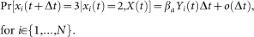


 , i.e.,
In above equations,  denotes probability,
  is the joint state of the network,
  is a time step and the indicator function 1{Q} is one if Q is true and zero otherwise. A function f (Δt) is said to be o(Δt) if limΔt→0 f (Δt)/Δt = 0. It is assumed that transition of an individual from an alert state to a susceptible state is much slower than other transitions. Hence, in the SAIS modeling setup, an alert agent never goes back directly to the susceptible state.
A common approach for studying a continuous-time Markov process is to derive the corresponding Kolmogorov forward (backward) differential equations (see28). As can be seen from the above equations, the conditional transition probabilities of a node are expressed in terms of the current state of its neighboring nodes. Therefore, each state of the Kolmogorov differential equations corresponding to the Markov process will be the probability of being in a specific joint state. In this case, we will end up with a set of first order ordinary differential equations of the order 3N. Hence, the analysis will become dramatically complicated as the network size grows. Using a proper mean-field-like approximation (see21,29), it is possible to express the transition probabilities in terms of infection probabilities of the neighbors. Hence, using this approximation, the differential equations (1) are derived.
References
Ferguson, N. Capturing human behaviour. Nature 446, 733 (2007).
Ferguson, N. M. et al. Strategies for mitigating an influenza pandemic. Nature 442, 448–452 (2006).
Funk, S., Salathe, M. & Jansen, V. A. A. Modelling the influence of human behaviour on the spread of infectious diseases: a review. Journal of The Royal Society Interface (2010).
Gonzalez, M. C., Hidalgo, C. A. & Barabasi, A.-L. Understanding individual human mobility patterns. Nature 453, 779–782 (2008).
Epstein, J. M. Modelling to contain pandemics. Nature 460, 687–687 (2009).
Sadique, M. Z. et al. Precautionary Behavior in Response to Perceived Threat of Pandemic Influenza. Emerging Infectious Diseases 13, 1307–1313 (2007).
Salathé, M. & Bonhoeffer, S. The Effect of Opinion Clustering on Disease Outbreaks. J. R. Soc. Interface 5, 1505–1508 (2008).
Kiss, I. Z., Cassell, J., Recker, M. & Simon, P. L. The impact of information transmission on epidemic outbreaks. Math Biosci 225, 1–10 (2010).
Reluga, T. C. Game Theory of Social Distancing in Response to an Epidemic. PLoS Comput Biol 6, e1000793 (2010).
Del Valle, S., Hethcote, H., Hyman, J. M. & Castillo-Chavez, C. Effects of behavioral changes in a smallpox attack model. Math Biosci 195, 228–251 (2005).
Wallinga, J., Edmunds, W. J. & Kretzschmar, M. Perspective: human contact patterns and the spread of airborne infectious diseases. Trends Microbiol. 7, 372–377 (1999).
Mossong, J. et al. Social Contacts and Mixing Patterns Relevant to the Spread of Infectious Diseases. PLoS Med 5, e74 (2008).
Garnett, G. P. & Anderson, R. M. Sexually Transmitted Diseases and Sexual Behavior: Insights from Mathematical Models. The Journal of Infectious Diseases 174, S150–S161 (1996).
SteelFisher, G. K., Blendon, R. J., Bekheit, M. M. & Lubell, K. The Public's Response to the 2009 H1N1 Influenza Pandemic. New England Journal of Medicine 362, e65 (2010).
Funk, S., Gilad, E., Watkins, C. & Jansen, V. A. A. The spread of awareness and its impact on epidemic outbreaks. Proceedings of the National Academy of Sciences 106, 6872 –6877 (2009).
Funk, S., Gilad, E. & Jansen, V. A. A. Endemic disease, awareness and local behavioural response. J. Theor. Biol. 264, 501–509 (2010).
Poletti, P., Caprile, B., Ajelli, M., Pugliese, A. & Merler, S. Spontaneous behavioural changes in response to epidemics. J. Theor. Biol. 260, 31–40 (2009).
Tracht, S. M., Del Valle, S. Y. & Hyman, J. M. Mathematical Modeling of the Effectiveness of Facemasks in Reducing the Spread of Novel Influenza A (H1N1). PLoS ONE 5, e9018 (2010).
Germann, T. C., Kadau, K., Longini, I. M. & Macken, C. A. Mitigation strategies for pandemic influenza in the United States. Proceedings of the National Academy of Sciences 103, 5935 –5940 (2006).
Perra, N., Balcan, D., Gonçalves, B. & Vespignani, A. Towards a Characterization of Behavior-Disease Models. PLoS ONE 6, e23084 (2011).
Sahneh, F. D. & Scoglio, C. Epidemic Spread in Human Networks. 50th IEEE Conference on Decision and Control (CDC) (2011).
Fenichel, E. P. et al. Adaptive human behavior in epidemiological models. Proceedings of the National Academy of Sciences 108, 6306 –6311 (2011).
Reluga, T. C. & Galvani, A. P. A general approach for population games with application to vaccination. Math Biosci 230, 67–78 (2011).
Van Segbroeck, S., Santos, F. C. & Pacheco, J. M. Adaptive Contact Networks Change Effective Disease Infectiousness and Dynamics. PLoS Comput Biol 6, e1000895 (2010).
Keeling, M. J. & Rohani, P. Modeling Infectious Diseases in Humans and Animals. (Princeton University Press: 2007).
Wu, Q., Fu, X., Small, M. & Xu, X.-J. The impact of awareness on epidemic spreading in networks. Chaos: An Interdisciplinary Journal of Nonlinear Science 22, 013101–013101–8 (2012).
Meloni, S. et al. Modeling human mobility responses to the large-scale spreading of infectious diseases. Scientific Reports 1, (2011).
Mieghem, P. V. Performance Analysis of Communications Networks and Systems. (Cambridge University Press: 2006).
Van Mieghem, P. The N-intertwined SIS epidemic network model. Computing 93, 147–169 (2011).
Chakrabarti, D., Wang, Y., Wang, C., Leskovec, J. & Faloutsos, C. Epidemic thresholds in real networks. ACM Trans. Inf. Syst. Secur. 10, 1:1–1:26 (2008).
Ganesh, A., Massoulie, L. & Towsley, D. The effect of network topology on the spread of epidemics. Proceedings IEEE INFOCOM 2005. 24th Annual Joint Conference of the IEEE Computer and Communications Societies 2, 1455–1466 vol. 2 (2005).
Gómez, S., Arenas, A., Borge-Holthoefer, J., Meloni, S. & Moreno, Y. Discrete-time Markov chain approach to contact-based disease spreading in complex networks. EPL (Europhysics Letters) 89, 38009 (2010).
Scoglio, C. et al. Efficient Mitigation Strategies for Epidemics in Rural Regions. PLoS ONE 5, e11569 (2010).
Acknowledgements
This work was supported by the National Agricultural Biosecurity Center (NABC) at Kansas State University. It was also based on work partially supported by the US National Science Foundation, while one of the authors, Fahmida N. Chowdhury, was working at the Foundation. Any opinion, finding and conclusions or recommendations expressed in this material are those of the authors and do not necessarily reflect the views of the National Science Foundation.
Author information
Authors and Affiliations
Contributions
F.D.S., F.C. & C.S. designed research, F.D.S., F.C. & C.S. performed research, F.D.S., F.C. & C.S. analyzed the data, F.D.S., F.C. & C.S. contributed new analytical results. All authors wrote, reviewed and approved the manuscript.
Ethics declarations
Competing interests
The authors declare no competing financial interests.
Rights and permissions
This work is licensed under a Creative Commons Attribution-NonCommercial-No Derivative Works 3.0 Unported License. To view a copy of this license, visit http://creativecommons.org/licenses/by-nc-nd/3.0/
About this article
Cite this article
Sahneh, F., Chowdhury, F. & Scoglio, C. On the existence of a threshold for preventive behavioral responses to suppress epidemic spreading. Sci Rep 2, 632 (2012). https://doi.org/10.1038/srep00632
Received:
Accepted:
Published:
DOI: https://doi.org/10.1038/srep00632
This article is cited by
-
Complexity of Government response to COVID-19 pandemic: a perspective of coupled dynamics on information heterogeneity and epidemic outbreak
Nonlinear Dynamics (2023)
-
Impacts of information propagation on epidemic spread over different migration routes
Nonlinear Dynamics (2021)
-
Mass Testing and Proactiveness Affect Epidemic Spreading
Journal of the Indian Institute of Science (2021)
-
Dynamic behaviour of competing memes’ spread with alert influence in multiplex social-networks
Computing (2019)
-
Oscillations in epidemic models with spread of awareness
Journal of Mathematical Biology (2018)
Comments
By submitting a comment you agree to abide by our Terms and Community Guidelines. If you find something abusive or that does not comply with our terms or guidelines please flag it as inappropriate.
