


« Prev Next »
Sampling Basics
Why we sample.
Recording every individual in a population is impractical, unnecessary, and expensive (Magurran 1988). Instead community ecologists and scientists in general take replicated samples to represent the overall community.
How many samples?
Too few samples can yield inaccurate and misleading results; too many becomes cost prohibitive (Eckblad 1991). Sample number is influenced by available resources, ethical concerns, and required accuracy. Detecting differences in parameters among sample groups depends upon parameter variability (Figure 1), and the size of the difference one is trying to detect (Gotelli & Ellison 2004). Gotelli & Ellison (2004) suggest the Rule of 10 as a minimum sample number per comparison category or treatment. Importantly, they point out that this rule cannot be universally applied, particularly with large-scale experiments.
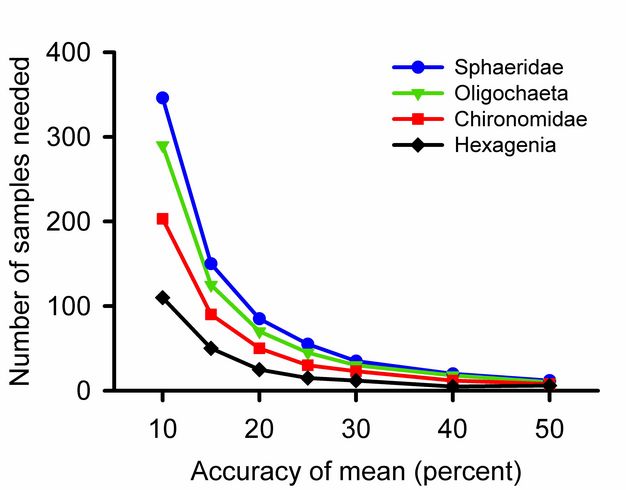
Figure 1
Number of samples needed to accurately estimate mean population densities of benthic macroinvertebrate species in the Mississippi River to within specified percentages. Species with more variable abundances in the samples required larger numbers of samples to provide accuracy. If reduced accuracy is acceptable for the question being addressed, then fewer samples can be used. Redrawn from Eckblad (1991).
© 2011 Nature Publishing Group All rights reserved. 
For most parameters a single sample provides an unbiased guess at the average. The first measured length of a nail, height of a person, or abundance of birds may be higher, lower, or equal to the true parameter. Adding samples increases the accuracy of a calculated average. Three is the minimum number of samples required for most statistical tests, but will not detect small differences among groups. Excellent community ecology has been done with five replicates per treatment or fewer. If one can take more replicates, however, the effort will reveal more subtle differences.
Keep individual samples separate.
It is essential keep samples separate. Don’t combine samples in a single container; don’t record several hours of bird observations on one tally sheet; keep data from separate transects in separate data columns. Composite data cannot be separated back into individual samples. Samples document the variability in the parameter of interest required for statistical tests. Each raw data set should be backed up in its original form. If combined samples are later required, one can sum samples copied from the raw data. One can calculate bird species observed per day by summing hourly data; but it is impossible to tell how many species occurred before 8:00 hrs from a daily total.
Diversity Sampling
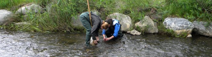
We will use published data, forest community data collected during General Biology by Saint Michael's College students, and benthic macroinvertebrate community data from Vermont EPSCoR’s Streams Project to illustrate principles of sampling biological communities. Benthic macroinvertebrate samples were collected by scrubbing rocks and agitating stream bed substrates. Student researchers collected the dislodged macroinvertebrates in a downstream net.
Samples underestimate community-wide richness.
Unlike typical samples, species richness in community samples will be less than the number of species in the sampled community. Community samples are biased if overall species richness is our parameter of interest. More samples or larger samples increases the number of species documented and always approaches the true parameter (S) from below. Connor & Simberloff (1978) analyzed plant community data from the Galapagos Islands and found that the number of botanical collecting visits per island better predicted species richness than did island area, elevation, or degree of isolation (Figure 2). In hyper-diverse assemblages such as arthropods, each sample potentially increases S with no end in sight.
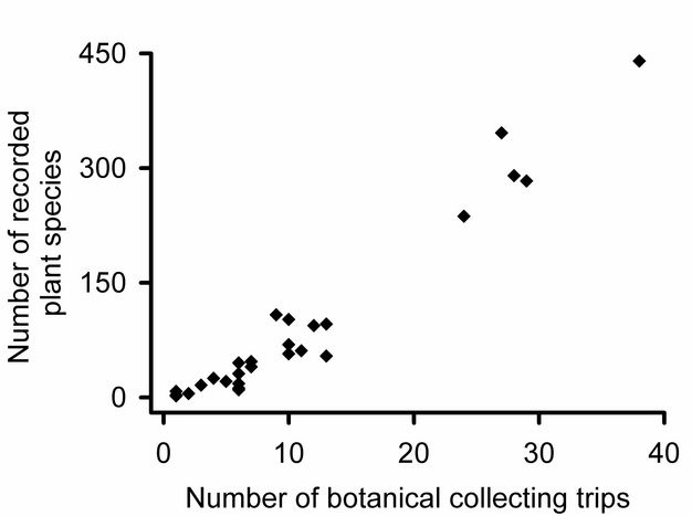
Figure 2
Illustrating the point that more sampling leads to more species observed. Connor & Simberloff (1978) analyzed data from collecting trips to the Galapagos Islands and found that number of collecting trips better explained number of species recorded than did island area, elevation, or isolation. Data extracted from Table 3 in Connor & Simberloff (1978).
© 2011 Nature Publishing Group All rights reserved.
How many community samples?
How many samples are needed depends on the goals. Diversity sampling often addresses two aims: 1) comparing sites or experimental treatments, and 2) estimating overall diversity. Samples taken to address aim 1, can later be combined to address aim 2. Overall diversity estimates improve as samples are added. However, even modest sampling efforts can detect diversity differences among habitats or treatments.
Sample-based comparisons.
What to record.
The minimum information in community samples is abundance of each taxon recorded. Taxon refers to species, genus, family, or some other operational taxonomic unit (OTU). Other variables such as gender and size may also be useful, but abundance of each OTU is an excellent starting point. For example, Saint Michael’s College students identified all trees taller than 1.4 m in 20 x 20 m quadrats in a recently burned forest and in a fire-suppressed control (Table 1). Importantly, the students recorded the abundance of each species. Species absent from a quadrat were indicated by a zero; a zero recorded represents a species not observed whereas blank cells may represent missing data.
|
Species |
Burned |
Control |
|
American beech |
1 | 0 |
|
Black cherry |
7 | 0 |
| Black oak | 0 | 1 |
|
Grey birch |
11 | 0 |
|
Pitch pine |
3 | 22 |
| Red maple | 0 | 35 |
| Red oak | 14 | 0 |
|
Service berry |
2 | 3 |
|
White oak |
0 | 3 |
|
White pine |
12 | 1 |
| Table 1. Numbers of trees greater than 1.4 m tall recorded by Saint Michael’s College students in 20 x 20 m quadrats in Camp Johnson in Colchester Vermont in September 2007. The ‘Burned’ treatment had been subjected to a controlled burn in 1998 and the ‘Control’ represents an adjacent fire-suppressed area. | ||
What are we measuring?
Diversity includes richness and evenness components (see Pyron 2010), but my focus will be on richness. To minimize confusion, the term abundance is reserved for the number of individuals rather than the number of species. Species density, the number of species per unit area, unit time spent observing, or per any technique-specific unit, is one of many indices calculated from community samples (see Magurran 1988). Measuring diversity from replicated samples provides a solid basis for comparisons among habitats, seasons, or experimental treatments.
Which community is more diverse?
Several community samples can be averaged to calculate the number of species expected per sample in a community or experimental treatment. Ling (2008) investigated spiny sea urchin impacts on Tasmanian marine invertebrates (Figure 3). His treatments included urchin removals, urchin-grazed plots (urchin barrens), and intact macroalgal plots. Richness in urchin barrens was lower than in intact macroalgal plots, or plots where urchin removal permitted macroalgal canopy recovery (Figure 3). Ling (2008) detected significant richness differences among treatments with just three replicate patches per treatment. The difference was detectable because of the large (four-fold) increase in species richness when urchins were removed.
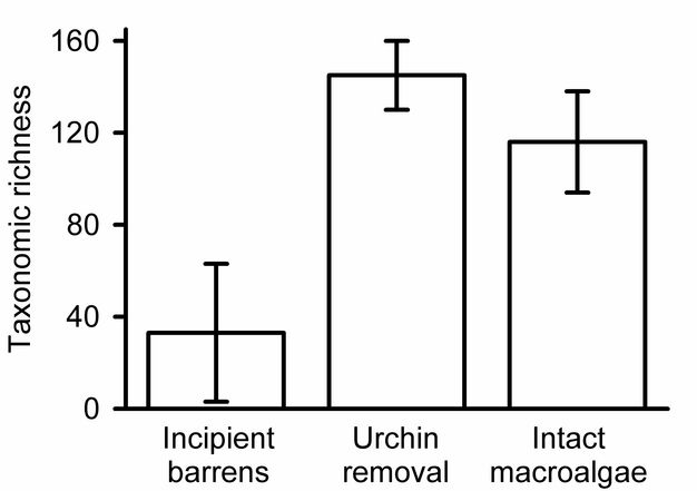
Figure 3
Benthic taxonomic richness in areas of heavy sea-urchin grazing (urchin barrens), areas where macroalgae had recovered following experimental urchin removal, and areas with naturally intact macroalgal communities. The averages were each calculated from 0.25 m2 quadrats and the error bars represent standard errors. Redrawn from Ling (2008).
© 2011 Nature Publishing Group All rights reserved.
Estimating and presenting overall diversity.
Replicate samples can be summed to arrive at an overall estimate of species richness, or the number of species that occur at a site, or set of treatments.
Confounded by abundance?
Abundance varies naturally and is further influenced by differences in sampling technique and effort. Richness differences can result from differences in the number of organisms sampled (Figure 2). In 2009 and 2010, Vermont EPSCoR Streams Project students collected macroinvertebrates from streams including Potash Brook, Centennial Brook (mixed urban watersheds) and Snipe Island Brook (forested watershed). Thirty nine macroinvertebrate families were recorded from Snipe Island Brook; 29 families from Potash Brook, and 10 families from Centennial Brook. But over 1,500 individual macroinvertebrates were sampled from two of the brooks while the Centennial Brook samples contained just 454 individuals. Are richness differences just sampling artifacts? The Snipe Island Brook and Potash Brook samples were quite comparable (1590 and 1543 individuals respectively). Having worked hard at identifying 454 macroinvertebrates, most scientists would like to be similarly comfortable comparing the Centennial Brook dataset! This common problem can be addressed using rarefaction (Simberloff 1972).
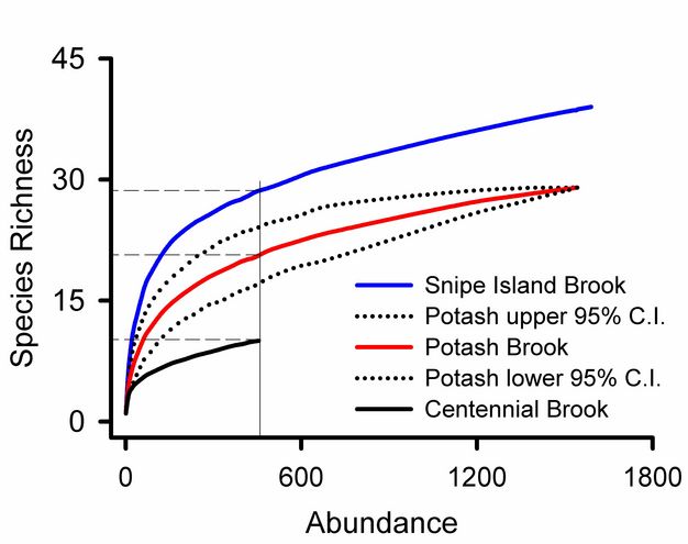
Removing abundance effects: Rarefaction.
Rarefaction answers the question "how many species would a smaller sample include?" The technique interpolates large samples for comparisons with smaller samples. Using free software (Gotelli & Entsminger 2009), we can repeatedly subsample 454 individuals from the 1590 macroinvertebrates collected from Snipe Island Brook and calculate the average number of families per subsample. The process can be repeated for multiple abundance levels. Resulting curves with abundance on the horizontal axis and taxonomic richness on the vertical axis (Figure 4) display the richness expected in sub-samples of any size. The 454 macroinvertebrates from Centennial Brook included 10 families. Subsamples of 454 individuals from larger samples included 17 families from Potash Brook, and 29 families from Snipe Island Brook. Adding 95% confidence limits to the Potash Brook curve, we can see that the number of families differs significantly from the other brooks.
Because diversity reflects richness and evenness, a number of other measurement and presentation approaches have been devised. Each approach has advantages that can reveal useful and interesting data patterns.
Figure 4
Solid lines are rarefaction curves of macroinvertebrate communities from three Vermont brooks. Dotted lines are 95% confidence limits of the Potash Brook curve. Just 454 individuals were sampled from Centennial Brook. The vertical line intersects each rarefaction curve at 454 individuals sampled; horizontal lines from those intersections show how many invertebrate families would be sampled if just 454 individuals were sampled from each brook.
© 2011 Nature Publishing Group All rights reserved.
Because diversity reflects richness and evenness, a number of other measurement and presentation approaches have been devised. Each approach has advantages that can reveal useful and interesting data patterns.
Collector’s curves.
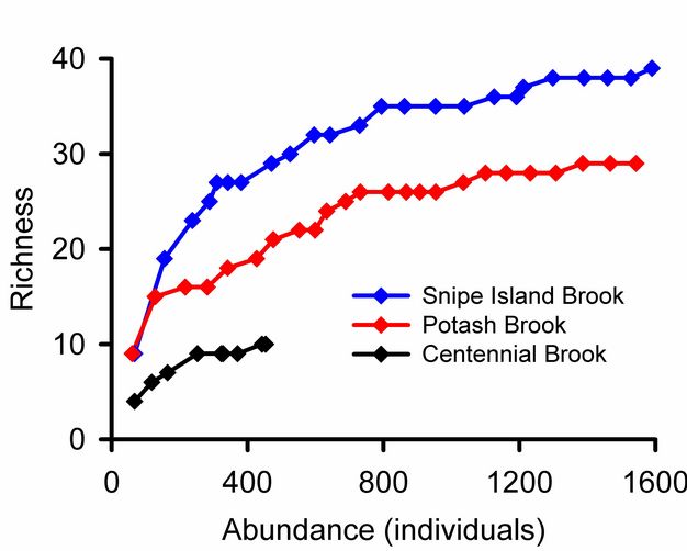
Adding multiple samples to a cumulative graph, with number of species on the vertical axis and abundance on the horizontal axis, generates a "collector’s curve" or "species accumulation curve" (Colwell & Coddington 1994; Figure 5). Graphing number of individuals on the horizontal axis is preferable to number of samples because varying sample sizes can distort the graph (Gotelli & Coleman 2001). Graphing numbers of individuals also facilitates comparisons with rarefaction curves (see above).
Collector’s curves rise rapidly when the relative abundances of the species are even (Gotelli & Coleman 2001). A sample from a community dominated by one species may contain only that dominant species and we might sample many individuals before observing more species. A collector’s curve would remain horizontal before very gradually stepping up as we record rare species. In even communities, early samples add more species and the graph steps up rapidly before leveling off when most species are accumulated. Unlike rarefaction curves that start at abundance = 1, richness = 1, collector's curves start at the abundance and richness of the first sample. Differences in shape between collector's curves and rarefaction curves reflect patchiness or non-randomness in the distributions of organisms in samples (Gotelli & Coleman 2001).
Rare species contribute uncertainty to all estimates of overall diversity. A collector’s curve illustrates this problem (Figure 5): it would be tempting to consider that the plateau in the Snipe Island Brook collector’s curve at 35 families represented a reasonably complete inventory of the groups present. Adding three more samples did not add a single new taxon. But the 17th sample added a new group, and three additional families were added by subsequent samples. The families added by later samples were rare groups missed by earlier samples and represented by just one or two individuals. The frequency of rare species relative to abundant species is used to assess confidence in overall estimates of taxonomic richness (Chao 1987). Lack of visual representation of the frequency of rare species is a weakness of collector’s curves addressed by log-normal plots illustrated below.
Figure 5
Collector’s curves from Vermont brooks. Taxonomic richness increases as samples are added. Each symbol represents a new sample; horizontal stretches of graph indicate that no additional families were added by samples. Differences in horizontal spacing of symbols reflect samples with different abundances. Curves from more even communities climb more rapidly.
© 2011 Nature Publishing Group All rights reserved.
Log-normal plots.
Natural community samples typically include a small number of very common species and a small number of very rare species. The majority of the species in the samples are moderately abundant. We can represent communities using a histogram with abundance categories on the horizontal axis and numbers of species in each category on the vertical axis. Preston (1948) plotted many such histograms using the log2 abundance scale and observed that many communities had a normal distribution of species–hence the lognormal distribution (Figure 6). Very common species (e.g., house mice) are in the right-hand tail of the histogram, while very rare species (e.g., large predators) are in the left-hand tail. In a well-sampled community we might expect most species to occur in the middle of the distribution. Even with extensive sampling, the very rarest species may remain undetected.
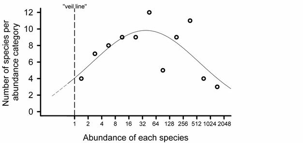
Preston’s (1948; Figure 6) analogy of a "veil line" described the discovery of rarer species by increasing the sampling effort. Early samples reveal the common species, while rare species remain hidden behind the imaginary veil line. Additional sampling shifts the veil line to the left. Thus, as rarer species are sampled and increases in abundance are recorded for each of the species already observed, the entire distribution is shifted to the right.
Using Preston’s (1948) approach we can see that uncertainty in our estimate of overall richness at Potash Brook is well justified (Figure 7). Seven families are represented by only one or two individuals: this is the largest category on the graph, suggesting that we can look forward to many additional days of sampling in Vermont to improve our estimate of taxonomic diversity (it could be worse). Additional sampling effort will increase the abundance of most species in our samples and probably yield previously unseen taxa.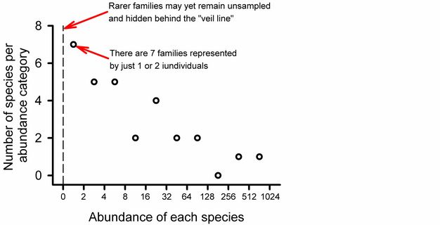
Figure 6
Preston’s (1948) log normal plot of Saunder’s breeding bird data. Four species are in the most abundant range with between 1024 and 2048 individuals recorded. Similarly, there are 4 species represented by 1 or 2 individuals. Most species are moderately abundant as indicated by the peak of the curve occurring near the 16-32 individuals observed range. Rarer species not yet observed remain hidden behind the “veil line”. Redrawn from Preston (1948).
© 2011 Nature Publishing Group All rights reserved.
Preston’s (1948; Figure 6) analogy of a "veil line" described the discovery of rarer species by increasing the sampling effort. Early samples reveal the common species, while rare species remain hidden behind the imaginary veil line. Additional sampling shifts the veil line to the left. Thus, as rarer species are sampled and increases in abundance are recorded for each of the species already observed, the entire distribution is shifted to the right.
Using Preston’s (1948) approach we can see that uncertainty in our estimate of overall richness at Potash Brook is well justified (Figure 7). Seven families are represented by only one or two individuals: this is the largest category on the graph, suggesting that we can look forward to many additional days of sampling in Vermont to improve our estimate of taxonomic diversity (it could be worse). Additional sampling effort will increase the abundance of most species in our samples and probably yield previously unseen taxa.
Figure 7
Unlike the example in Figure 6, this plot peaks at the left, indicating that rare families are quite common. This suggests that additional sampling is warranted to more thoroughly represent the community.
© 2011 Nature Publishing Group All rights reserved.
Rank abundance curves.
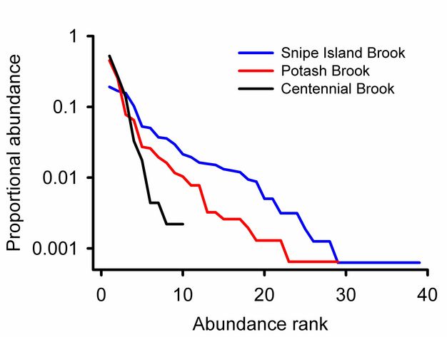
Ranking species from most abundant to least provides another useful way to visualize community data. Using proportions allows for comparisons of samples of different sizes. Plotting on a log scale allows for better data visualization. Rank abundance curves are plotted with rank from most abundant to least on the horizontal axis; log of proportional abundance is on the vertical axis. The last data point corresponds to the number of species observed; the first point shows the degree to which the community is dominated by the most abundant species. The slope of the declining graph indicates evenness with more even communities producing flatter graphs.
Rank abundance curves for Vermont streams (Figure 8) show that Snipe Island Brook has more families than Centennial Brook and that the relative abundances of those species are more evenly distributed. We can also see that 0.52 of the individuals from Potash Brook are from a single taxon. The most abundant family in Snipe Island Brook represents 0.19 of the community.
Rank abundance curves for Vermont streams (Figure 8) show that Snipe Island Brook has more families than Centennial Brook and that the relative abundances of those species are more evenly distributed. We can also see that 0.52 of the individuals from Potash Brook are from a single taxon. The most abundant family in Snipe Island Brook represents 0.19 of the community.
Figure 8
Rank abundance curves for contrasting Vermont brooks. Centennial Brook drains mixed urban areas, is impacted by runoff from impervious surfaces, and has just 10 macroinvertebrate families sampled. Snipe Island Brook drains forested land and has 40 macroinvertebrate families sampled. The steeper curve from Centennial Brook indicates a very uneven distribution of relative abundances of the families collected. Potash Brook drains mixed land uses and was sampled downstream from a wooded area. It is of intermediate species richness and evenness.
© 2011 Nature Publishing Group All rights reserved.
Summary
Appropriately-collected community data can be presented in a number of useful ways to reveal patterns, address questions, and make comparisons. Data collected to compare sample-scale questions and treatments can later be combined to address habitat-wide questions. Sampling effort and differential abundance of individuals in samples affects the number of species observed. Rarefaction of data can separate sampling artifacts from real patterns in community data.
References and Recommended Reading
Chao, A. Estimating the population size for capture-recapture data with unequal catchability. Biometrics 43, 783–791 (1987).
Colwell, R. K. & Coddington, J. A. Estimating terrestrial biodiversity through extrapolation. Philosophical Transactions of the Royal Society B: Biological Sciences 345, 101–118 (1994).
Connor, E. F. & Simberloff, D. Species number and compositional similarity of the Galapagos flora and avifauna. Ecological Monographs 48, 219–248 (1978).
Eckblad, J. W. How many samples should be taken? Bioscience 41, 346–348 (1991).
Gotelli, N. J. & Colwell, R. K. Quantifying biodiversity: Procedures and pitfalls in the measurement and comparison of species richness. Ecology Letters 4, 379–391 (2001).
Gotelli, N. J. & Ellison, A. M. A Primer of Ecological Statistics. Sunderland, MA: Sinauer & Associates, 2004.
Gotelli, N. J. & Entsminger, G. L. Ecosim: Null models software for ecology. Version 7.0. Jericho, VT: Acquired Intelligence Inc. & Kesey-Bear, 2009. (link)
Ling, S. Range expansion of a habitat-modifying species leads to loss of taxonomic diversity: A new and impoverished reef state. Oecologia 156, 883–894 (2004).
Magurran, A. E. Ecological Diversity and its Measurement. Princeton, NJ: Princeton University Press, 1988.
Preston, F. W. The commonness, and rarity, of species. Ecology 29, 254–283 (1948).
Pyron, M. Characterizing communities. Nature Education Knowledge 1, 20 (2010).
Simberloff, D. Properties of the rarefaction diversity measurement. The American Naturalist 106, 414–418 (1972).