


« Prev Next »

The physical properties of seawater include both 'thermodynamic properties' like density and freezing point, as well as 'transport properties' like the electrical conductivity and viscosity. Density in particular is an important property in ocean science because small spatial changes in density result in spatial variations in pressure at a given depth, which in turn drive the ocean circulation.
Physical properties can be measured directly. However, direct measurements can be complicated to carry out, especially in the field, and in many cases it is more convenient to measure a few important 'state variables' on which the properties depend, and then look up the desired property as a function of the measured state in a table, or calculate it using a mathematical formula. The table or formula that is used is usually derived from careful laboratory measurements. Such a table or formula, when formally defined in a published document and endorsed by a scientific authority, is known as a standard.
Physical properties vary with the amount of heat and the amount of dissolved matter contained in the water, as well as the ambient pressure. Important state variables measured for parcels of water in the ocean are therefore temperature, which is related to the heat content, salinity, which is related to the amount of dissolved matter, and the pressure (Table 1). In addition to controlling physical properties, the variation in space and time of temperature and salinity are also important water mass tracers that can be used to map the ocean circulation. Density is usually calculated using a mathematical function of temperature, salinity, and pressure, sometimes called an equation of state. For many years the internationally accepted standard for seawater densities has been the 1980 International Equation of State, known by the acronym EOS-80. However, a new international standard for seawater density, as well as all other thermodynamic properties, has recently been developed. This new standard is called the Thermodynamic Equation of Seawater (2010), or TEOS-10. In turn, standards like EOS-80 or TEOS-10 rely on other international standards that precisely define the state variables of temperature and salinity. Standards thus play an important role in ocean science.
| Variable | Ocean Range | Ocean Mean | Required Accuracy |
| Temperature | -2°C to 40°C | 3.5°C | ±0.002°C |
| Absolute Salinity | 0 g/kg to 42 g/kg | 34.9 g/kg | ±0.002 g/kg |
| Pressure | 0 dbar to 11000 dbar | 1850 dbar | < ±3 dbar |
| In-situ Density | 1000 to 1060 kg/m3 | 1036 kg/m3 | ±0.004 kg/m3 |
| Table 1. Ocean state variables, their typical ranges and mean values in the ocean, and the accuracy to which they are measured (or estimated) in the deep ocean. Pressures in the ocean are usually measured in dbar (decibars), with values offset to read zero at the surface. Pressure values expressed in this way are numerically similar (within 2%) to depth in meters below the surface. That is, the pressure at a depth of 1000 meters is about 1000 dbars. | |||
Temperature
What is temperature? This is more difficult to define than it first appears. A textbook definition (the Zeroth Law of Thermodynamics) says:
"There exists a scalar quantity called temperature, which is a property of all thermodynamic systems (in equilibrium states) such that temperature equality is a necessary and sufficient condition for thermal equilibrium."
As a corollary to this definition, objects in contact with one another will tend toward thermal equilibrium by an exchange of heat between them. Thus, if we know the temperature of one object (call it a thermometer), and it is in thermal equilibrium with water around it, which will occur after enough time has passed, we also know the temperature of the water. Conversely, if water and a thermometer within it are at different temperatures, then there must be a flow of energy (heat) between the water and the thermometer. This gives us both a way of talking about energy and a way of measuring temperature using a known reference.
In turn, the temperature of the thermometer can be related to its physical properties. These physical properties include the volume-to-mass ratio of a solid, liquid, or gas, or the electrical resistance of a metal or a semiconductor. Temperature can therefore be determined through direct measurements of these properties.
But how do we define a numerical scale for temperature, as measured by our thermometer? The simplest way is to define two reference points, plus a method that can be used to interpolate between them. In 1742, Anders Celsius defined a temperature scale in which the freezing point of water (at sea-level pressure) was taken as a lower reference point with a value of 0, with the difference between the freezing point and the boiling point (also at sea level pressure) taken as 100 units, measured in terms of the change in volume of a fluid.
As time went on, more and more precisely specified definitions (or standards) for temperature became necessary as scientific questions required intercomparing more and more accurate observations of temperature. However, in order to preserve a historical continuity, these redefinitions were usually formulated in such a way as to allow easy comparison with older observations. We therefore still use the °C as a unit of temperature, and water still freezes at about 0°C and boils at about 100°C, although temperature scales are no longer defined in terms of the freezing and boiling points of water.
An important step in the history of temperature occurred in the 1800s, when the concept of temperature gained a theoretical backing with the development of the science of thermodynamics. William Thomson (who later became Lord Kelvin) suggested a thermodynamic temperature scale in which the ratio of temperatures above an 'absolute zero' would be in proportion to the heat absorbed and rejected by a theoretical construct called a Carnot cycle engine, operating between these two temperatures.
A thermodynamic scale is thus implicitly referenced to a lower limit of absolute zero, which is defined to be 0K (kelvin). The freezing point of water was chosen to be a second reference. By numerically defining the temperature of the freezing point of water to be 273.15K, the thermodynamic temperature of the boiling point is found to be 373.15K, 100 units higher, so that an interval of 1K and 1°C are identical.
However, determining thermodynamic temperature is very difficult, and for most applications more practical methods are needed. These practical definitions of temperature generally rely on fixing the values of certain reference points based on careful measurements of their thermodynamic temperatures, and then specifying a way of interpolating between them. Points at which different phases of particular materials co-exist are useful reference points. However, rather than boiling and freezing points (which depend on the ambient pressure), better fixed points occur at the triple points of different substances. A triple point is the single unique combination of temperature and pressure at which solid, liquid, and gas phases of a particular substance can all coexist.
The current standard for temperature is the International Temperature Scale (1990), or ITS-90. In ITS-90, temperatures in the range of oceanographic interest are set by:
1. the triple point of mercury, defined to be ≡ -38.8344°C exactly
2. the triple point of pure water with a specified isotopic composition, defined to be ≡ 0.01°C (or 273.16K) exactly
3. the melting point of gallium, defined to be ≡ 29.7646°C.
In addition, a method of calculating temperatures between these reference points is also described by ITS-90. Such temperatures are interpolated using a specified polynomial function of the measured electrical resistance of a platinum wire. Temperatures outside the oceanographic range are defined using other fixed points and methods of interpolation.
Temperatures specified using the previous international standard temperature scale (the International Practical Temperature Scale 1968 or IPTS-68) differ from ITS-90 by up to 0.01°C over the range of oceanographic interest. Although our normal day-to-day activities usually don't require accuracies of more than about 0.1°C at best, a difference of 0.01°C is somewhat larger than the accuracy to which deep ocean measurements are now made (Table 1). Careful adherence to standards is therefore necessary to allow us compare measurements made by different people around the world, and to compare contemporary measurements to measurements made in the past and in the future.
Although in-situ temperature t defined by ITS-90 is generally the quantity we measure, it is not the most useful variable for describing heat content itself. Two effects can cause problems. First, the energy required to change the temperature of seawater by a fixed amount (say, 1°C), called the heat capacity, is itself a function of temperature and salinity. It takes about 5% less energy to heat average seawater by 1° C than it does to heat the same mass of freshwater by 1°C. Second, the effects of pressure can act to change the in-situ temperature of water without changing the heat content. Squeezing typical seawater (or air) causes the temperature to rise. A pressure of 100 atmospheres (or about 1000 dbar) is enough to increase measured seawater temperatures by about 0.1°C. However, the temperature of near-freezing fresh water actually falls as pressure increases.
To account for the pressure effects, a variable called potential temperature, denoted θ, is traditionally used in oceanography. The potential temperature of a water parcel is the temperature that would be measured if the water parcel were enclosed in a bag (to prevent the loss or gain of any salt) and brought to the ocean surface adiabatically (i.e., without exchanging any heat with its surroundings). The potential temperature is therefore insensitive to pressure by definition, but is lower than the in-situ temperature by about 0.1°C for every 1000 m of depth increase (Figure 1a).
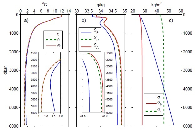
Figure 1: A vertical profile of temperature and salinity at 39°N, 152°W in the North Pacific (data courtesy of the CLIVAR and Carbon Hydrographic Data Office, cchdo.uscd.edu).
a) Vertical profiles of in-situ temperature t, potential temperature θ, and Conservative Temperature Θ. Inset shows an expanded view of deep ocean values. Potential and Conservative temperature are within 0.0003°C in the deep ocean. Note that heat content (proportional to Θ) actually decreases with depth, but pressure effects cause a rise in the in-situ temperature t. b) Vertical profiles of Practical Salinity SP (with no units), Reference Salinity SR, and Absolute Salinity SA. c) Vertical profiles of in-situ density (σ), potential density referenced to the sea surface (σθ), and potential density referenced to 4000 dbar (σ4). Most of the in-situ density increase with depth is due to pressure effects, which are removed in the calculation of potential densities, showing how weakly stratified the ocean actually is.
© 2013 Nature Education All rights reserved. 
However, potential temperature does not account for the varying heat capacity of seawater, and is therefore not a conservative measure of heat content. A variable is conservative if its value in a mixture of two parcels of seawater is the average of its values in the two initial parcels. Conservative variables are very useful in making budgets. Although the heat content of a mixture of two seawaters is the average heat content of the two, both the in-situ and potential temperature of a mixture can differ from the average temperature of the two initial parcels.
A different type of temperature, defined in TEOS-10, more precisely scales with heat content and is for all practical purposes conservative, as well as insensitive to pressure. It is called Conservative Temperature, and denoted Θ. Conservative Temperature differs from potential temperature by as much as 1°C for warm fresh waters, but is usually well within ±0.05°C for most ocean waters (Figure 1a).
Although the differences between these different types of temperature are small, they can be significantly larger than the precision to which temperature measurements of the ocean are routinely reported (Table 1). It is therefore important to make clear which temperature is under consideration in any discussion.
Salinity
Salinity is a measure of the ‘saltiness' of seawater, or more precisely the amount of dissolved matter within seawater. Operationally, dissolved matter is that which remains after passing the seawater through a very fine filter to remove particulate matter. Historically, a glass fiber filter with a nominal pore size of 0.45 μm was used. More recently, filters with 0.2 μm pores have become standard, since filters with this pore size will catch the smallest bacteria.
However, the history of the salinity concept, and its various definitions (which have changed over time) is a long and complex story, dating back to the late 19th century. The story is complex for two reasons. First, any useful definition of salinity contains approximations of some kind. These approximations are necessary because the dissolved matter in seawater is a complicated mixture of virtually every known element and it is impossible to measure the complete composition of every water sample. Second, subtle technical details of these approximations, which have undergone changes as more has been learned about seawater, are very important in practice. These details are important because the required measurement accuracy for salinity, necessary to understand the ocean general circulation, is extremely high (about ±0.006%, see Table 1), so that even small changes in numerical values can have significant implications if incorrectly interpreted.
Most useful definitions of salinity are rooted in the well-known fact that the relative ratios of most of the important constituents of seawater are approximately constant in the ocean (the Principle of Constant Proportions). Therefore, practical but approximate measures of the total dissolved content can be found by scaling measurements of a single property.
Originally the property most conveniently measured was the chlorinity, or halide ion (mainly Cl-and Br-) concentration. Chlorinity was measured using a straightforward chemical titration, and then converted to a measure of salinity using a simple linear function. Such salinities can often be identified by an attached unit of ppt, or the symbol ‰.
However, almost all modern estimates of salinity rely on measurements of the electrical conductivity (or, at high precision, on measurements of the ratio of the conductivity of a sample of seawater to the conductivity of a special reference material called IAPSO Standard Seawater). Since the electrical conductivity of seawater is also highly temperature-dependent, and mildly pressure-dependent, temperature and pressure must also be measured in this approach. The conversion from measured temperature, pressure, and conductivity to salinity is complex and nonlinear. Since the early 1980s, oceanographers have used a calculated value formally called the Practical Salinity (denoted SP) as a proxy for true salinity. Practical Salinity is defined as a function of temperature, pressure, and conductivity by another standard, the Practical Salinity Scale 1978 (or PSS-78). When oceanographers use the word salinity they often mean Practical Salinity, although it is better to use the full name to prevent ambiguity.
It is important to emphasize that Practical Salinities do not have units. This fact, confusing to non-specialists, is related to technical issues that prevented an absolute definition when PSS-78 was constructed. Sometimes this lack of units is awkwardly handled by appending the acronym PSU (Practical Salinity Units) to the numerical value, although doing so is formally incorrect and strongly discouraged. Practical Salinities are numerically smaller by about 0.5% than the mass fraction of dissolved matter when this mass fraction is expressed as grams of solute per kilogram of seawater. Practical Salinities were, however, defined to be reasonably comparable with numerical values of chlorinity-based salinities, to maintain a historical continuity.
The special reference material used to calibrate salinity instruments, IAPSO Standard Seawater, is manufactured by a single company (Ocean Scientific International Ltd., UK) and is created using seawater obtained from a particular region of the North Atlantic. Although the use of Standard Seawater to determine Practical Salinity has been routine for many years, the dependence of Practical Salinity measurements on a physical artifact known to degrade with age leads to a number of technical problems, especially in terms of the long-term stability and intercomparability of high-precision ocean measurements.
The new seawater standard TEOS-10 defines a better measure of the salinity, called Absolute Salinity (denoted SA). This new definition incorporates several features designed to address the technical difficulties discussed above and provides the best available estimate of the mass fraction of dissolved matter. It is usually associated with an attached unit of g/kg.
First, the definition of salinity is no longer based on properties of IAPSO Standard Seawater. Instead, the best estimates of the concentrations of the important inorganic components of Standard Seawater are used in TEOS-10 to exactly define an artificial seawater with Reference Composition (Table 2). For practical and historical reasons, the definition of Reference Composition ignores dissolved organic matter, as well as most gases, although it otherwise includes the most important constituents in real low-nutrient seawater.| Reference Composition | mmol/kg | mg/kg |
| Na+ |
468.9675 |
10781.45 |
| Mg2+ |
52.8170 |
1283.72 |
| Ca2+ |
10.2820 |
412.08 |
| K+ |
10.2077 |
399.10 |
| Sr2+ |
0.0907 |
7.94 |
| Cl- |
545.8695 |
19352.71 |
| SO42- |
28.2353 |
2712.35 |
| Br- |
0.8421 |
67.29 |
| F- |
0.0683 |
1.30 |
| HCO3- |
1.7178 |
104.81 |
| CO32- |
0.2389 |
14.34 |
| B(OH)3 |
0.3143 |
19.43 |
| B(OH)4- |
0.1008 |
7.94 |
| CO2 |
0.0097 |
0.43 |
| OH- |
0.0080 |
0.14 |
| Observed Variations seen in real seawater | ||
| O2 |
0 - 0.3 |
0 - 10 |
| N2 |
0.4 |
14 |
| Si(OH)4 |
0 - 0.17 |
0 - 16 |
| NO3- |
0 - 0.04 |
0 - 2 |
| PO4- |
0 - 0.003 |
0 - 0.2 |
| ΔCa+ |
0 - 0.1 |
0 - 4 |
| ΔHCO3- |
0 - 0.3 |
0 - 20 |
| Dissolved Organic Matter (DOM) |
– |
0 - 2 |
| Table 2. Reference Composition of seawater with SP ≡ 35.000 and SR ≡ 35.16504 g/kg. Concentrations in seawater of higher or lower salinities can be found approximately by scaling all values up or down by the same factor. Units of concentration are per kilogram of seawater. Real seawater contains additional constituents which are not included in the Reference Composition but whose concentrations (and their variation) may be larger than 1 mg/kg. Concentrations of these constituents do not increase or decrease with salinity but are largely controlled by biogeochemical processes. | ||
Next, a numerical Reference Salinity (denoted SR) is defined, representing the mass fraction of solute in this Reference Composition seawater. Reference Salinity has units of grams of solute per kilogram of seawater, and is numerically determined by multiplying the concentrations of the different components of the Reference Composition by their atomic weights, and then summing. Salinities defined in this way are said to lie on the Reference Composition Salinity Scale. Note that uncertainty in the atomic weights themselves contributes an uncertainty of about 1 mg/kg to this definition.
Standard Seawater is now treated as a physical artifact that approximates Reference Composition Seawater. A particular sample of Standard Seawater is then assigned a Reference Salinity on the Reference Composition Salinity Scale. This Reference Salinity is numerically different from the Practical Salinity of the sample (Figure 1b), but it can be obtained from the conductivity-based Practical Salinity using a simple scaling. However, Reference Salinity can also be estimated using other approaches (e.g., by direct measurements of density and inversion of the TEOS-10 equation of state).
Although the definition of the Reference Composition provides a standard for the definition of the salinity of Standard Seawater, when considering real seawaters an additional problem arises. This is because the relative chemical composition of seawater is in fact slightly different in different geographic locations. The most important variations that occur in the real ocean arise from changes in the carbon system, and in the concentrations of Calcium (Ca2+) and the macronutrients nitrate (NO3-) and silicic acid (Si(OH)4) (Table 2). These constituents are affected by biogeochemical processes in the ocean. They are removed by the formation of biological material, and returned by its dissolution.
When using PSS-78 these changes in relative composition are ignored. However, this means that waters of the same Practical Salinity, from different parts of the ocean, may contain different mass fractions of dissolved matter. The difference can be as large as 0.025 g/kg in the open ocean (Figure 1b). In coastal waters, where the presence of river salts is an additional factor, the difference can be as large as 0.1 g/kg. Differences of this size are more than an order of magnitude larger than the precision to which salinity is reported (Table 1).
Under TEOS-10 these changes in the relative composition are explicitly accounted for in the definition of Absolute Salinity. The TEOS-10 Absolute Salinity can be determined by first measuring the electrical conductivity, temperature, and pressure of a water parcel, as before. Then Reference Salinity is calculated as if the water had Reference Composition. Finally, a small correction factor is added to account for the compositional variations. This correction, also known as the salinity anomaly, is denoted ΔSA. It is roughly correlated with the concentration of macronutrients in seawater, and is largest in the deep North Pacific, where these concentrations are greatest.
Density
The most important thermodynamic property of seawater for studies of oceanic circulation is its density (denoted ρ). Typical densities span a narrow range (Table 1, Figure 1c).
It is therefore conventional in discussions of the ocean to use a derived variable σ for density, where
σ = ρ/(kg/m3 ) - 1000
so that the leading '10', virtually always present in numerical values of density, is dropped. For example, a density of 1027.534 kg/m3 would usually be written as a σ-value of 27.534 kg/m3.
Density depends on heat content and salinity. Since seawater is not perfectly incompressible, it also varies slightly with pressure. The variation of σ with Conservative Temperature and Absolute Salinity can be illustrated using a T-S diagram, or more properly a Θ-SA diagram (Figure 2). A water parcel with a particular Θ and SA is plotted as a point in such a diagram. By calculating the density at all possible points (keeping pressure fixed at a specified value), and contouring the calculated values, isopycnal lines can be drawn on the diagram joining together different combinations of temperature and salinity that result in the same density.
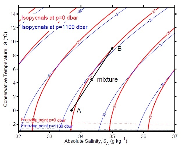
Figure 2: This Θ -SA diagram can be used to illustrate relationships between temperature, salinity, and density for different water masses.
Lines of constant σ are contoured at the surface (red curves for p = 0 dbar), and at about 1100 m depth (blue curves, p = 1100 dbar). Near the surface water masses A and B, with different temperatures and Absolute Salinities, both have σ ≈ 27 kg/m3, with the density of water A slightly less than the density of water B. However, at 1100 dbar where σ ≈ 32 kg/m3 water mass A is more dense than water mass B.
© 2013 Nature Education All rights reserved.
As one would expect, more saline waters at a particular temperature are more dense. Increasing the Absolute Salinity by about 1 g/kg increases density by about 0.8 kg/m3. However, isopycnal lines joining water types of different temperature and salinity but the same density are not straight. Instead, they are curved, with a right-facing concavity. The curvature of the isopycnals shows that the effects of temperature on density are very much greater in warm waters (i.e., near the surface in the tropics) than they are in cold waters found at depth and in the polar regions.
However, there is always a small temperature effect, and so the isopycnal curves never become vertical for seawaters with salinities typical of the open ocean. Although maximum densities occur at temperatures of around 4°C for fresh waters, for Absolute Salinities greater than 23.8 g/kg, seawaters at the freezing point are most dense. Freezing temperature also decreases with salinity, with typical seawater freezing at around -1.9°C at atmospheric pressure.
The curvature of the isopycnals gives rise to a phenomenon known as cabbeling, or a contraction on mixing. Consider two water masses, A and B, with different Conservative Temperature and Absolute Salinity, which are plotted at different locations on the Θ-SA diagram (Figure 2). Water mass A is fresher, but colder, than water mass B. However, near the surface when pressure is 0 dbar, the density of each water mass is less than or equal to 1027 kg/m3, as the points representing these water masses are on or left of the 27 kg/m3 isopycnal (red curves in Figure 2). The Conservative Temperature and Absolute Salinity of a mixture of two water masses will lie along the straight line (the 'mixing line') joining them in this diagram. However, the curvature of the isopycnals means that the density of this mixture may be to the right of the 27 kg/m3 isopycnal (i.e., its density may be greater than 1027 kg/m3). This increase in density is important in the Southern Ocean. There, different water masses on the surface can be brought together by ocean currents. The parcels mix, and after mixing together, the denser mixed water that results sinks below the surface.
If we draw this diagram at higher pressures (e.g., blue curves in Figure 2), the general features remain the same, but quantitative aspects can change. An obvious change is that the freezing temperature decreases with pressure. Thus meltwater from the base of thick Antarctic ice shelves, which is at the freezing point at depth when pressures are high, can become supercooled after rising upwards in the water column. Such waters are difficult to measure as instruments lowered into them rapidly become coated in ice crystals. Also, as pressure increases, the isopycnals do not remain in the same place in the diagram. Instead, densities increase with pressure and the isopycnal curves move leftwards. Isopycnals calculated at a pressure of 1100 dbar show that densities for a given Θ and SA are about 5 kg/m3 higher than they are at the surface.
This increase in density with pressure is a problem when trying to decide which of two water parcels in the ocean, initially at different depths, would be lighter than the other if they were brought together. This is because the pressure effects often result in the largest apparent differences (Figure 1c). Instead of comparing the in-situ densities, it is more useful to compare the densities as if both parcels are brought adiabatically to the same reference pressure. When this reference pressure is taken to be at the surface, the resulting measure of density is called potential density, denoted σθ.
However, in addition to generally moving leftwards as pressure increases, the isopycnals on this diagram also rotate slightly. The isopycnals calculated at 1100 dbar are tilted rightward relative to those calculated at 0 dbar. The density of warmer waters does not increase quite as much as the density of colder waters for the same change in pressure. Thus, two water parcels with different temperatures and salinities but the same density at the surface (i.e., with the same potential density) will in fact have slightly different densities at another depth even if their heat content and salinity remain the same. This is called the thermobaric effect. In deep convection areas, which are places in the Labrador and Greenland seas, and in some locations around Antarctica where surface water is cooled and eventually sinks to depths of several thousand meters, the thermobaric effect can be important in accelerating downward convection, resulting in large vertical displacements in the position of water parcels.
On the other hand, the rotation of isopycnals can also lead to mistakes in the interpretation of potential density. Consider water parcels A and B in Figure 2 again. Near the surface, parcel B is slightly more dense than parcel A. However, at 1100 dbar, parcel A is slightly more dense than parcel B. If we are trying to decide which of the two water masses is heavier at depths near 1100 dbar, then comparing potential densities will give an incorrect answer. This difficulty is an important factor in correctly understanding water characteristics near the bottom of the South Atlantic. There, waters with larger potential density are observed to lie above waters with smaller potential density, which at first glance suggests a large-scale instability. However, the shallower water mass is heavier than the deeper water mass only if both are brought to the surface. If both are brought to the ocean bottom, the shallower water mass is lighter than the deeper water mass and one can conclude that the water column is stably stratified.
When comparing different water masses it is therefore best to minimize the effects of this isopycnal rotation. Thus, when comparing different water masses near, say, 4000 m (especially in the South Atlantic), typically densities are pressure-corrected to exactly 4000 dbar rather than to the surface. The resulting potential density referenced to 4000 dbar is denoted as σ4 (Figure 1c). Deciding which measure of density to use in oceanographic analyses can be challenging, and is still an area of ongoing research.References and Recommended Reading
The main reference to TEOS-10, and the details of how conservation of energy (i.e. the First Law of Thermodynamics) is handled in the ocean, is the manual:
IOC, SCOR and IAPSO, The international thermodynamic equation of seawater - 2010: Calculations and use of thermodynamic properties. Intergovernmental Oceanographic Commission, Manuals and Guides No. 56, UNESCO (English), 196 pp. (2010). http://www.teos-10.org along with software and other information.
Complete details of ITS-90 are in
- Preston-Thomas, H., The International Temperature Scale of 1990, Metrologia 27, 3-10, (1990).
Additional information
about ITS-90 is given at http://www.its-90.com.
PSS-78 and EOS-80 are described in two special reports (that are mostly a compendium of journal articles):
- UNESCO, Background papers and supporting data on the Practical Salinity Scale 1978, UNESCO Technical Papers in Marine Science 37, 144 pp. (1981).
- UNESCO, Background papers and supporting data on the International Equation of State of Seawater 1980, UNESCO Technical Papers in Marine Science 38, 192 pp. (1981).
Many of the intricate details involved in PSS-78 are also found in the articles contained in:
Special Issue on the Practical Salinity Scale 1978, IEEE J. Oceanic Engineering 5, 1-62 (1980).
More details on the actual composition of sea and river waters, and their effects on various methods of determining density and/or salinity can be found in:
- Millero, F.J., Chemical Oceanography, Boca Raton Fl: CRC Press, (2005).
Basic information about thermodynamic temperatures and the Carnot cycle can be found in any introductory physics text, e.g.
- Halliday D., and R. Resnick, Fundamentals of Physics, Wiley, (various editions and years).
Less technical articles describing the people and history behind some of the scientific issues related to seawater salinity and density can be found at:
- Pawlowicz, R. et al.. An historical perspective on the development of the Thermodynamic Equation of Seawater - 2010, Ocean Sci. 8, 161-174, (2012).
- Millero, F. J., History of the Equation of State of Seawater, Oceanography 23(3), 18-33, (2010).