


« Prev Next »
Agricultural crops are regularly infested with insect pests whose population size can reach outbreak densities in some years, causing considerable income loss to farmers. In general, the risk of pest outbreaks is highest when insects disperse to crop fields early in the growing season and the population growth rate is high. The population growth rate measures how much the population size (i.e., number of individuals of a species in a defined area) changes per unit time. Suites of natural enemies (predators and parasitoids) prey upon insects and thereby reduce the risk of pest insects causing economically significant damage. The most common tool for farmers to control pest insects is the application of insecticides. However, unnecessary insecticide applications incur costs to purchase and use and may increase future pest problems by killing beneficial insects. Scientists can help farmers avoid unnecessary insecticide applications using mathematical models to predict future pest population sizes. Predicting future population sizes and evaluating what factors are most critical for population growth are also essential to other areas in ecology such as invasive species management and conservation ecology.
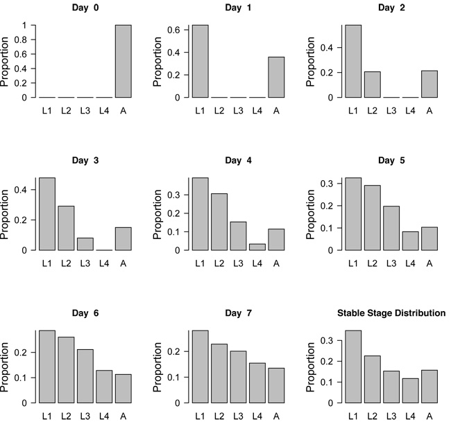
Figure 1: Projected population structure of aphids following a dispersal event on Day 0.
Once the stable stage distribution is reached, the relative proportion of each developmental stage remains constant. L1 = first larval stage, L2 = second larval stage, L3 = third larval stage, L4 = fourth larval stage, A = adult stage.
© 2010 Nature Education All rights reserved. 
Populations consist of individuals that differ in age, size, or developmental stage (e.g., the relative proportion of eggs, juveniles, and adults). The distribution of individuals among these categories is known as the stage distribution of the population. The stage distribution influences the population growth rate and varies through time. Interestingly, if environmental conditions remain constant long enough, the stage distribution settles into a particular pattern in which the relative proportion of the different stages remains constant over time. This is called the "stable stage distribution." Imagine some adult aphids disperse to an alfalfa field in the spring (Figure 1). Initially the population consists of only adult aphids (Day 0). As soon as the adults give birth, the population consists of adults and newborn aphids (Day 1). Aphid larvae have four juvenile stages, called instars, through which they develop to become adults; newborn aphids are in the first instar. By Day 2, some first instar aphids have grown enough to molt and become second instar larvae; at the same time, more first instar larvae are born. By Day 4, the aphid population consists of all four juvenile stages and the adult stage, but the relative proportion of stages still changes for some time. If nothing else changes, the population eventually reaches the stable stage distribution and the speed at which the population is growing approaches a constant rate (the asymptotic population growth rate). This means that although the proportion of individuals in each stage is constant, the total population is still growing at a constant rate. However, while the stage distribution is changing, the population growth rate may be completely different (Figure 2).
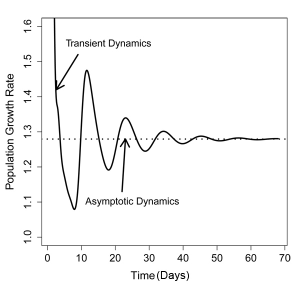
Figure 2: Projected population growth rates
The solid line refers to a population that consists of 100% adults on Day 0 as depicted in Figure 1. The dotted line indicates a population that is at the stable stage distribution on Day 0 (lower right panel in Figure 1).
© 2010 Nature Education All rights reserved.
When Are Short-Term (Transient) Dynamics Important?
The fluctuations in population growth rate following the dispersal event are known as transient dynamics because the fluctuations do not persist. In the past, ecologists focused on studying the long-term dynamics, or asymptotic dynamics, assuming that populations have been around for long enough to approach a stable stage distribution. However, there is an increasing awareness that many populations experience disturbances, like fire or drought, which push the population away from the stable stage distribution. For instance, after a wildfire, all adults of a fire intolerant species die, and all that is left are the seeds in the seed bank. Although the plant population will resume growing after a fire, it may take several years before the population reaches the stable stage distribution again. If the interval between fires is shorter than the time required to reach the stable stage distribution, the population dynamics may be better described by transient dynamics.
Transient population dynamics may also play an important role for species exploiting ephemeral resources, such as pioneer plants that frequently colonize new areas. The population growth rate during the early phase of a colonization event influences the likelihood of successful establishment. The founder population is initially highly skewed toward the dispersal stage (like seeds or seedlings for plants or adults for many animal species) and typically consists of only a few individuals. Small populations have a high inherent risk of extinction because of Allee effects and demographic stochasticity; therefore, the transient population growth rate determines how quickly a founder population remains in the stage of dangerously small numbers.
In general, transient dynamics are expected after any disturbance (biotic or abiotic) that causes a deviation from the stable stage distribution. Examples include flood or drought which may have different impacts on each life history stage. For example, newborns may be more likely to die in a drought than adults or large grazers moving temporarily through an area that have a preference for young, juicy plants. In contrast, we do not expect transient dynamics if the biotic or abiotic factors are consistently present, such as specialist predators that reliably consume seeds every year; their impact on plant demography is already incorporated into the stable stage distribution.
Mathematical Models
Both transient and asymptotic dynamics can be predicted using stage-structured population models. This type of model does not assume all members of a population have similar vital rates; instead, it tracks the abundance of individuals that differ in age or size. Life history parameters like survival and fecundity often depend on age or size. Stage-structured population models are a widely used tool to examine the importance of different life history stages for the asymptotic population growth rate. For instance, this type of analysis might inform population mangers whether limited resources should be spent to manipulate juvenile survival or adult reproduction to reach a desired population size in the future. There are several different types of stage-structured models. The types most commonly used by ecologists involve matrix population models. It is much simpler to analyze asymptotic population dynamics in these models. For example, there is a single formula calculating how quickly a population grows assuming asymptotic dynamics; in contrast, studying transient dynamics involves computer simulations. How wrong will our predictions of future population size be if we ignore the occurrence of transient dynamics?
Transient dynamics may be important for many aphid species because they exploit ephemeral resources. Aphid populations typically crash three to four generations after dispersing to their host plants (Dixon & Agarwala 1999) because host plant quality decreases with time and the pressure of natural enemies increases. My colleagues and I (Tenhumberg et al. 2009) used a matrix population model of pea aphids to compare predicted trajectories of populations that started out with 100% adults (adults are the dispersal stage of aphids) or with populations that started out at the stable stage distribution. Transient dynamics are expected in the former and asymptotic dynamics in the latter scenario.
Transient dynamics may be important for many aphid species because they exploit ephemeral resources. Aphid populations typically crash three to four generations after dispersing to their host plants (Dixon & Agarwala 1999) because host plant quality decreases with time and the pressure of natural enemies increases. My colleagues and I (Tenhumberg et al. 2009) used a matrix population model of pea aphids to compare predicted trajectories of populations that started out with 100% adults (adults are the dispersal stage of aphids) or with populations that started out at the stable stage distribution. Transient dynamics are expected in the former and asymptotic dynamics in the latter scenario.
Pea Aphids Experiments
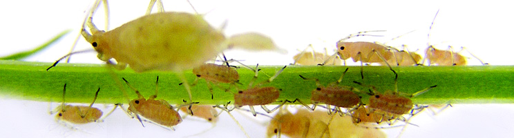
From spring to autumn pea aphids (Acythosiphon pisum) reproduce asexually (parthenogenetically) and give birth to live young. The newborn aphids go through four juvenile instars before molting to the adult stage. We estimated growth, survival, and fecundity rates by rearing single aphids from birth to death in clip cages that were fastened onto alfalfa leaves (Figure 3). This single individual gave rise to a population of aphids through asexual reproduction of young. Every day we checked if the aphids were still alive and whether they had molted to the next instar. Once they were adults, we counted the number of newborns. Newborn aphids were removed from the clip cages each day. We found that aphids stay about two days in each juvenile stage, and only 13% of them died before reaching adulthood. Young adults gave birth to an average of 3.4 newborns within a 24-hour period. Aphid birth rate dropped and the risk of dying increased with age. On average, adult aphids died after two weeks (see Tenhumberg et al. 2009 for a more detailed description of the results of the experiments).
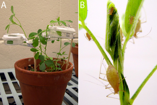
Figure 3: Pea aphid (Acyrthosiphon pisum) experiment
(A) Clip cages are fastened onto alfalfa leaves. (B) There is a single aphid in each cage feeding on the phloem of alfalfa plants and individual aphids can be observed from birth to death.
© 2010 Nature Education 3B courtesy of Masaru Takahashi. All rights reserved.
Pea Aphid Model
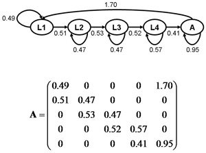
Figure 4: Pea aphid population projection model
The upper graph illustrates an aphid life cycle graph. L1–L4 denote the first through fourth instars and A stands for adults. The arrows denote all possible transitions between stages, and the corresponding transition rates are listed next to the arrow. For instance, only adults can produce first instar larvae and on average a single adult produces 1.7 offspring each day. This model assumes that all first instar larvae survive. Each day, on average 51% of the first instar larvae molt to the second instar and the rest (51%) remain first instar lavae. These transition rates can be summarized in form of a population projection matrix as illustrated in the lower graph. Some transitions are biologically impossible like changing from a second instar to a first instar larvae or juveniles reproducing; these transitions appear as zeros in the matrix.
© 2010 Nature Education All rights reserved.
Estimating the future size of a population that starts out from any other stage distribution involves simulations. For this, we divided the population N0 into the different stages: in our "dispersal scenario," we assumed all individuals of N0 belong to the "young adult" stage, and the number of individuals in all other stages was zero. In our equilibrium scenario, all individuals were distributed among the different stages according to the stable stage distribution. For instance, if for a population of N0 equals 100 individuals in the stable stage distribution 35% of the population is in the first instar, then the first instar stage would get 35 individuals. The number of individuals in the different stages were entered into a starting population vector n(t = 0). Then we simulated the population trajectories of both scenarios using this formula: n(t + 1) = An(t). From one day to the next (from t to t+1) the number of individuals in the different stages changed; and so did the total population size (the sum of the number of individuals in the different stages). Figure 4 provides a generic example of a population projection matrix.
Simulation Results
We then plotted the predicted population trajectories of both scenarios on a log scale (Figure 5). In the equilibrium scenario, the population grew at a constant rate, which is a straight line when plotted on a log scale; the slope of this line equals the population growth rate. In contrast, in the dispersal scenario, the population growth rate fluctuated and, particularly during the first few days the population growth rate, was much higher (steeper) slope than in the equilibrium scenario. After about twenty days, the population trajectories became parallel (i.e., at this point the population growth rates of both scenarios were about the same and both populations were at the stable stage distribution). We then calculated the transient amplification, Tr, after twenty days (roughly two aphid generations) by dividing the population size of the dispersal scenario by the population size of the equilibrium scenario (Figure 3). The transient amplification was 3.05, which means that after twenty days, the population that started out with only adults was three times as high as a population that started out at the stable stage distribution. Thus, ignoring the stage distribution of pea aphids early in the season results in a significant underestimation of future population size.
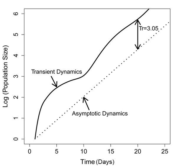
Figure 5: Projected population trajectories: Population sizes are plotted on a log scale
The solid line refers to a population that consists of 100% adults on Day 0 (scenario 1), and the dotted line indicates a population that is at the stable stage distribution on Day 0 (scenario 2). Tr = Nscenario1/Nscenario2 — where N refers to the population size in the two different scenarios on Day 20.
© 2010 Nature Education Adapted from Tenhumberg, B. et al. Model complexity affects predicted transient population dynamics following a dispersal event: a case study with Acyrthosiphon pisum. Ecology 90,1878–1890 (2009). All rights reserved.
Other Pitfalls
When predicting future population sizes it is necessary to watch out for not only transient dynamics but also models with insufficient complexity. For example, models that ignored the effect of aphid senescence (older aged aphids have a lower birth rate and a higher chance of dying) did not predict transient fluctuations in population growth rates. In another set of laboratory experiments, we mimicked the dispersal of adult aphids into an alfalfa field and recorded the change in population size for twenty days (Tenhumberg et al. 2009). We documented fluctuations in the population growth rates which were consistent with the predictions of a model that included the effect of aphid senescence.
Conclusions
In undisturbed environments, the population structure of animal and plant populations approaches a stable stage distribution and the population size changes at a constant rate (asymptotic dynamics). Some events can cause a temporal change in the population structure and population growth rate (transient dynamics). Examples for such events include dispersal to new environments or habitat patches and irregularly occurring abiotic and biotic disturbances like fire, drought, flooding and predation. The magnitude of the difference between transient and asymptotic dynamics depends on how far the population structure deviates from the stable stage distribution and the details of the life history (specified in the population projection matrix A).
References and Recommended Reading
Caswell, H. Matrix Population Models, 2nd ed. Sunderland, MA: Sinauer & Associates, 2001.
Dixon, A. F. G. & Agarwala, B. K. Ladybird-induced life-history changes in aphids. Proceedings of The Royal Society B 266,1549–1553 (1999).
Tenhumberg, B. et al. Model complexity affects predicted transient population dynamics following a dispersal event: a case study with Acyrthosiphon pisum. Ecology 90,1878–1890 (2009).