


« Prev Next »
During the most recent ice ages of the Quaternary (the last 2.6 million years), continental ice sheets covered much of Canada, the northern United States, northern Europe, and extended into the Arctic Ocean, with the Antarctic Ice Sheets growing to the continental shelf break (Figure 1) (Clark & Mix 2002). The growth and decay of these ice masses drove sea-level fluctuations on the order of 10's to over 100 m on the time scales of 100's to 10,000 years (Figure 2d) (Lambeck & Chappell 2001, Rohling et al. 2009). Periods where sea-level was >10 m below present are typically referred to as glacial periods; the intervening periods with sea level close to present day are called interglacial periods. The most rapid and dramatic periods of sea-level rise occurred during major deglaciations when most Northern Hemisphere ice sheets disappeared and the Greenland and Antarctic Ice Sheets retreated to their present extents. Essentially, Earth switched from a glacial to an interglacial state. The frequency of deglaciations is approximately every 100,000 years for the last 500,000 years (Figure 2d). During at least one of the interglaciations, sea level was several meters higher than present, indicating retreat of at least one of the three remaining ice sheets to a smaller than present extent (Kopp et al. 2009, Rohling et al. 2009).
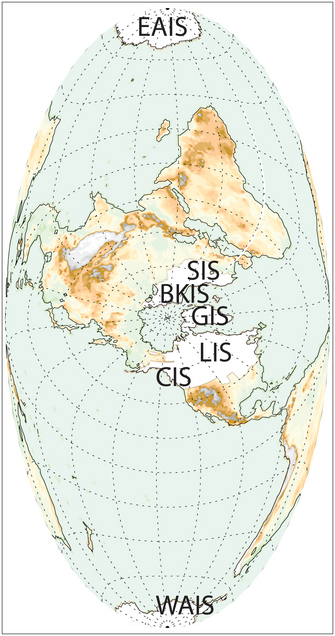
Figure 1
Extent of the Laurentide (LIS), Cordilleran (CIS), Greenland (GIS), Barents-Kara (BKIS), Scandinavian (SIS), and West (WAIS) and East (EAIS) Antarctic Ice Sheets at the Last Glacial Maximum (~21 ka) (Peltier 2004, Clark et al. 2009).
The fluctuations between glacial and interglacial states are driven by changes in Earth's orbit around the sun - called Milankovitch Cycles - that change the amount of incoming solar radiation called insolation (Figure 2a) (Hays et al. 1976, Berger & Loutre 1991). Because the major changes in Earth's ice masses occurred in the Northern Hemisphere where much of the Earth's land surface presently resides, it is hypothesized that high-northern latitude, or boreal, summer insolation was the most important forcing of the glacial-interglacial cycle. Ice sheets respond to both changes in precipitation (snow) and summer temperature with cold, wet conditions favoring ice growth and warm, dry conditions ice retreat. Ice sheets seem to mainly respond to changes summer temperature, which is what is affected by the Milankovitch cycles (e.g., Imbrie et al. 1993), with precipitation playing a lesser role in governing the growth and decay of ice.
Indeed, each of the major deglaciations depicted in Figure 2 correspond with an increase in boreal summer insolation. However, the relationship between sea level and boreal summer insolation is not one-to-one, and many increases in insolation do not have corresponding deglaciations. The lack of a direct correlation between insolation and sea level implies that Milankovitch Cycles may have additional influences on ocean circulation and atmospheric CO2 concentration, which amplify the effects of the changes in insolation, a process known as a positive feedback (Figures 2b & c) (Imbrie et al. 1993). Thus the Earth's climate system tends to force a persistent glacial state until a threshold is crossed-such as ice sheets extending too far south-and a deglaciation occurs in response to the next increase in boreal summer insolation (Imbrie et al. 1993, Clark et al. 1999). This article discusses the evidence for how ice sheets responded to these periods of past natural deglacial climate warming and contributed to sea-level rise, focusing on the last deglaciation and last interglaciation (Figure 2) for which sufficient data exist to discern the behavior of individual ice sheets.
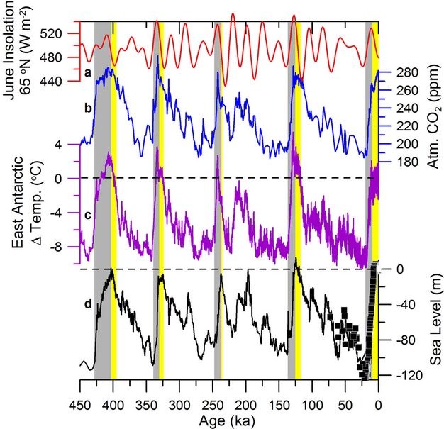
Figure 2: Climate and sea level of the last 450 kyrs.
(a) June insolation at 65° N, the driving force behind the growth and decay of ice sheets (Berger & Loutre 1991). (b) Atmospheric CO2 concentrations from Antarctic ice cores, a positive feedback on ice-sheet growth and decay (Siegenthaler et al. 2005). (c) East Antarctic change in temperature with dashed line denoting present day temperature (Jouzel et al. 2007). (d) Sea-level records from the Red Sea (black line) and individual sea-level estimates (black squares), with dashed line denoting present-day sea level (Clark et al. 2009, Rohling et al. 2009). Gray bars indicate deglaciations; yellow bars indicate interglaciations.
Methods of Monitoring Ice-Sheet Behavior
The major late Quaternary ice sheets are the Laurentide (LIS), Cordilleran (CIS), Scandinavian (SIS), Barents-Kara (BKIS), Greenland (GIS) and East (EAIS) and West (WAIS) Antarctic Ice Sheets (Figure 1), which can be divided into predominately terrestrial and marine-based ice sheets. Terrestrial ice sheets, such as the LIS, CIS, SIS, GIS, and EAIS, have their margins and ice-base resting and terminating on land. That said, portions of these ice sheets, and the entire GIS and EAIS margins, did terminate in the ocean. Marine-based ice sheets like the BKIS and WAIS have much of their ice-base resting on ground below sea level, with their ice margin terminating in the ocean. This type of ice-sheet may be unstable because a rise in sea level, or thinning of the ice sheet, could trigger a destabilization where parts of the ice sheet could float, break up and rapidly retreat, which is often referred to as a collapse.
The combined behavior of global ice volume is recorded by fluctuations in sea level. The rise and fall of sea-level can be reconstructed by radiometrically dating corals who's habitat is near the sea surface and using their present elevations above or below current sea level as indicators of past sea-level fluctuations (Figure 2d) (e.g., Lambeck & Chappell 2001). Another method is to document changes in the salinity of evaporative basins only marginally connected to the open ocean, such as the Red Sea. A fall in sea level increases the influence of evaporation on the basin and the isotope ratio of the heavy 18O to light 16O increases in surface dwelling (planktonic) foraminifera shells (Figure 2d), because the lighter 16O is preferentially evaporated and not replenished by the reduced in low of ocean water (Siddall et al. 2003, Rohling et al. 2009). A third means of reconstructing sea level-usually applicable to time scales longer than discussed here-is the use of the 18O to 16O relationship in bottom dwelling (benthic) foraminifera (amoeboid animals) shells (e.g., Hays et al. 1976, Imbrie et al. 1993). Due to preferential evaporation of lighter 16O from the global ocean, this isotope accumulates in ice sheets and thus the ratio of 18O to 16O increases in the ocean during periods of ice growth. Similarly, the retreat of ice releases the sequestered 16O back to the ocean, reducing the 18O/16O ratio. This ratio is commonly expressed against a known standard of 18O/16O and denote using the symbol δ (i.e., δ18O).
The history of individual ice sheets can be determined directly by dating ice margin retreat and ice surface thinning, and indirectly from inferences of ice sheet runoff to the ocean. Radiocarbon (the radioactive isotope of C; 14C) dates on organic matter or calcite shells indicate the absence of ice, and with a significant number of ages bracketing glacial deposits, the advance and retreat of ice can be reconstructed (e.g., Landvik et al. 1998, Dyke 2004, Clark et al. 2009). Ice-sheet retreat can be directly dated using cosmogenic isotope ages of boulders deposited by the ice. Retreat exposes these boulders to the bombardment of cosmic radiation from outer space (fast protons, neutrons, and electrons) that impact upon elements in the rock's crystals, splitting or attaching to the atoms to make new isotopes (i.e., 3He, 10Be, 14C, 21Ne, 26Al, 36Cl) (Gosse & Phillips 2001). With a known production rate of these isotopes, one can calculate how long a boulder has been exposed to this bombardment by measuring the concentration of the isotope in the boulder surface. The melting of ice during retreat increases the discharge of 16O water to the ocean where the δ18O will decrease in planktonic foraminifera, allowing inference of greater ice retreat (Jones & Keigwin 1988). The runoff from ice-sheet melting will also transport more sediment to the ocean, which can be tracked by analyzing marine sediments for the abundance of terrestrially-derived elements such as Ti and Fe (Carlson et al. 2008b).
The retreat of ice sheets can be compared with ice core O and H isotope records of the ice (H2O). The δ18O of precipitation decreases as atmospheric temperatures cool because the colder air causes more of the 18O to be precipitated out of the cloud, leaving behind a lower 18O to 16O ratio that is recorded in the ice core. Warming causes the opposite effect. The 2H isotope called Deuterium behaves in a similar manner with the more common 1H isotope. Their ratio relative to a standard is denoted as δD. With a known linear relationship between δ18O and δD (e.g., Cuffey et al. 1995, Jouzel et al. 2007), ice core records can be converted into changes in temperature.
The Last Deglaciation
The last deglaciation spanned ~20-6 ka (ka=kilo annum, or a thousand years before present) with sea level rising 125-130 m (Figure 3g) reflecting the retreat of all of the Earth's ice sheets. Sea-level rise was not constant, however, with increases above its average rate of rise of ~1 cm yr-1 at 20-19, ~14.5 and 11-8 ka that resulted in many meters of sea-level rise in the span of centuries (Figure 3f), suggesting periods of rapid retreat of one or more of these ice sheets (Figure 1). The first increase in the rate of sea-level rise at 20-19 ka to ~1.4 cm yr-1 followed shortly after the initial rise in boreal summer insolation (Figure 3a) (Yokoyama et al. 2000, Clark et al. 2004). Terrestrial 14C and cosmogenic records and marine runoff records indicate that retreat had commenced for all Northern Hemisphere ice sheets by 20-19 ka in rapid response to rising boreal summer insolation and causing this acceleration in sea-level rise (Figures 3c-e) (Clark et al. 2009). However, terrestrial and marine ice sheets reacted differently to this initial increase in the incoming energy from the sun. The retreat of the terrestrial LIS slowed following this rise in sea level as indicated by its 14C-dated ice margin chronology (Figure 3e). In contrast, the marine BKIS rapidly retreated, or collapsed, as suggested by a significant decrease in δ18O (Jones & Keigwin 1988) with 14C dates indicating that much of its mass was gone before ~15 ka (Figure 3c) (Landvik et al. 1998).
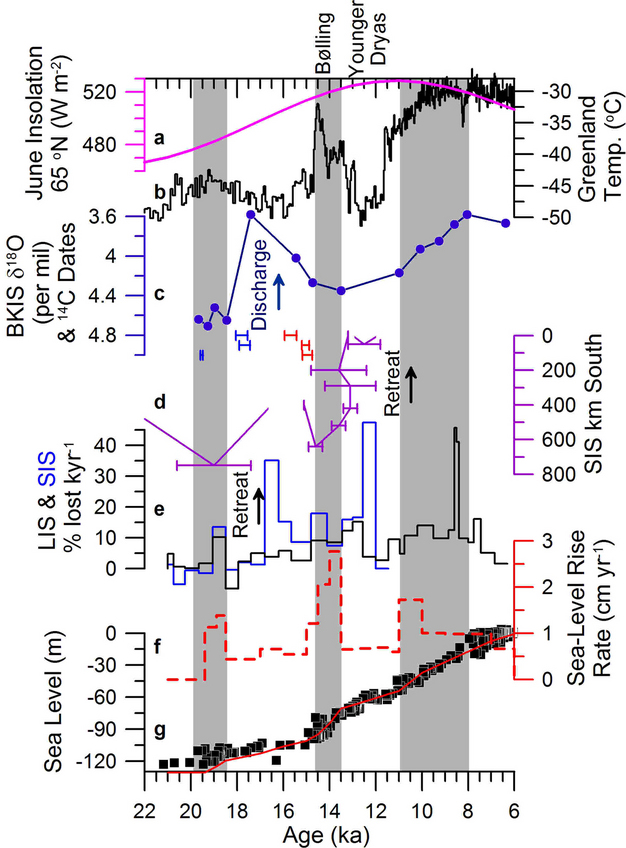
Figure 3: Records of Northern Hemisphere ice sheets during the last deglaciation.
(a) June insolation at 65° N (Berger & Loutre 1991). (b) Greenland temperature based on ice core oxygen isotopes (δ18O) converted to temperature (Cuffey et al. 1995). (c) A record of BKIS discharge based on planktonic δ18O (Jones & Keigwin 1988). Lower isotope values indicate more ice-sheet discharge from retreat ~18 ka (note the lighter isotopes after ~12 ka reflect warming, not ice sheet retreat). Also shown are radiocarbon (14C) dates that indicate BKIS retreat starting 20–18 ka (blue bars) and when the ice sheet was essentially gone 16–15 ka (red bars) (Landvik et al. 1998). (d) Distance south of the southern SIS relative to its extent ~12 ka as determined by cosmogenic isotope dates on glacial boulders (Rinterknecht et al. 2006). The bars indicate the uncertainty in the timing of each ice position. (e) Rate of LIS (black) and CIS (blue) retreat based on the percent of their area lost per kyr reconstructed by 14C dates (Dyke 2004). Note that the abrupt increase in CIS retreat ~12.5 ka is an artifact of rapid thinning up to ~13 ka that exposed the underlying mountains and greatly reduced the area of the CIS. (f) Rate of sea-level rise (Clark et al. 2009). (g) Sea level from individual estimates (black squares) and a sea-level model (red line) (Clark et al. 2009). Gray bars show periods of rapid sea-level rise discussed in text. The Bølling and Younger Dryas are also indicated.
The next deglacial increase in the rate of sea-level rise is called Meltwater Pulse (MWP) 1A (Fairbanks 1989) and occurred roughly coincident with warming of the North Atlantic region into what is termed the Bølling warm period ~14.6 ka (Figure 3b). During MWP-1A, sea level rose at the fastest rate of the last deglaciation, approaching ~2.8 cm yr-1. The LIS has long been assumed to be the main source of MWP-1A with additional contributions from the other Northern Hemisphere ice sheets (Fairbanks 1989, Peltier 2004, Tarasov & Peltier 2005). However, retreat rates of the LIS, CIS and SIS (Figure 1) as indicated by 14C and cosmogenic dates did not accelerate until after MWP-1A. Rather they responded gradually to Bølling warming (Figures 3d & e) with retreat slowing for the LIS and SIS during the subsequent cold period called the Younger Dryas (Figure 3b) (~12.9-11.7 ka) (Dyke 2004, Rinterknecht et al. 2006). Furthermore, δ18O records of meltwater discharge suggest <1/2 of MWP-1A came from the LIS and SIS (Clark et al. 1996, Carlson 2009, Obbink et al. 2010). Given that the BKIS was already well retracted (Figure 3c), an additional source of sea-level rise is required to explain the abruptness and magnitude of MWP-1A.
Several lines of evidence point towards contributions from the marine-based portions of the WAIS and EAIS. Ice margin 14C and cosmogenic dates indicate the onset of WAIS deglaciation 15-14 ka (Figure 4c) (Johnson et al. 2008, Clark et al. 2009, Bentley et al. 2010, Todd et al. 2010). An abrupt increase in ice core δD could record this rapid thinning as warming due to a drop in ice surface elevation (Price et al. 2007). The marine and potentially terrestrial portions of the EAIS also began retreat before ~14 ka (Mackintosh et al. 2011, White et al. 2011). This onset of WAIS and EAIS retreat occurred after an extended period of Antarctic warming (Figure 4b), implying that the marine portions of this ice-sheet responded abruptly, or non-linearly, to a gradual forcing.
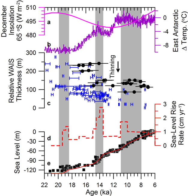
Figure 4: Records of Antarctic ice retreat.
(a) December insolation at 65° S (Berger & Loutre 1991). (b) East Antarctic change in temperature (Jouzel et al. 2007). (c) Records of WAIS thinning near the Ross Sea relative to present elevation. Blue bars are dates that constrain the level of a lake dammed by the WAIS against the Transantarctic Mountains of the Ross Sea region (Hall & Denton 2000). Higher lake levels exist prior to 15–14 ka from ice at its maximum height. The permanent drop in lake level by ~14 ka indicates abrupt thinning of the WAIS. The black circles are cosmogenic dates that constrain the elevation of the ice surface that flowed into the Ross Sea with a significant drop in ice elevation ~14.5 ka (Todd et al. 2010). (d) Rate of sea-level rise (Clark et al. 2009). (e) Sea level from individual estimates (black squares) and a sea-level model (red line) (Clark et al. 2009). Gray bars show periods of rapid sea-level rise discussed in text.
The Last Interglaciation
The last interglaciation occurred ~128-116 ka (Shackleton et al. 2003) and followed a significantly more rapid deglaciation than the last deglaciation, likely forced by a greater increase in boreal summer insolation than the last deglaciation (Figure 2) (Ruddiman et al. 1980, Oppo et al. 1997, Siddall et al. 2006, Carlson, 2008). Boreal temperatures were 0-5 °C warmer than the late Holocene (CAPE 2006). Interestingly, ice-core records suggest significant warming over the EAIS upwards of 6°C despite a minimum in austral summer insolation (Figures 2c & 5c) (e.g., Jouzel et al. 2007, Sime et al. 2009). During this interglaciation, sea level rose to at least 4 m higher than present ~126-120 ka at rates approaching 1 cm yr-1 (Figures 2d & 5d) (Rohling et al. 2008, Kopp et al. 2009). The two most likely sources of the higher sea level are the GIS and WAIS, which would raise sea level ~7 and 3.3 to 5 m, respectively, upon complete deglaciation (Mercer 1978; Overpeck et al. 2006, Bamber et al. 2001, 2009).
Terrestrial and marine records indicate the GIS was diminished in size during the last interglaciation, although the magnitude of retreat is not well known and debated. Ice-core δ18O records suggest little change in the elevation of the ice surface relative to present in north Greenland, because the gradient in δ18O between different ice cores was roughly the same as at present (NGRIP 2004). However, significant thinning, but not complete deglaciation may have occurred in the south of Greenland because ice-core δ18O was much higher than at present, suggesting the ice surface was significantly lower than at present (NGRIP 2004, Willerslev et al. 2007). Alternatively, these same ice-core records have been interpreted to indicate almost complete deglaciation of southern Greenland (Otto-Bliesner et al. 2006, Alley et al. 2010) and significant retreat in northern Greenland (Koerner & Fisher 2002). Ice-sheet model simulations also estimate a wide range in GIS retreat, predicting sea-level rise contributions between ~1.6 and 5.5 m (Cuffey & Marshall 2000, Huybrechts 2002, Tarasov & Peltier 2003, Lhomme et al. 2005, Otto-Bliesner et al. 2006). Marine records of GIS runoff as inferred by increases in terrestrial sediment discharge to the ocean indicate a significantly longer period of elevated melting and greater retreat during the last interglaciation relative to the early Holocene (Stoner et al. 1995, Carlson et al. 2008b). A protracted period of elevated GIS runoff from ~128 to 120 ka suggests continued GIS retreat through this interglaciation with a minimum extent ~120 ka (Figure 5b). Pollen that drifted to the ocean from southern Greenland denotes greater vegetation development on Greenland relative to the Holocene, also supporting greater ice retreat (de Vernal & Hillaire-Marcel 2008).
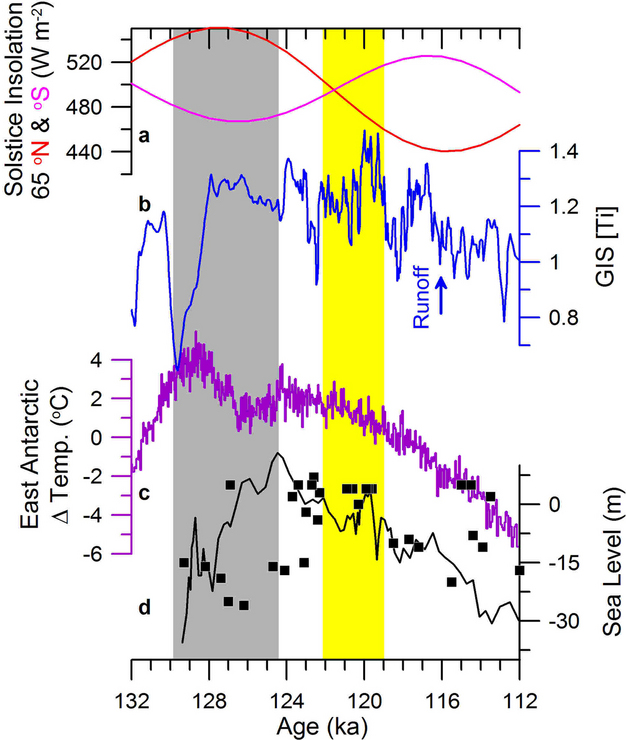
Figure 5: Last interglacial records.
(a) June and December insolation at 65° N (red) & S (purple) (Berger & Loutre 1991). (b) Runoff of the southern GIS based on the concentration of Ti in marine sediments (Carlson et al. 2008b). More Ti indicates more terrestrial sediment discharged to the ocean from the GIS. (c) East Antarctic change in temperature (Jouzel et al. 2007). The warmer than present interval during the first half of the last interglaciation may indicate collapse of the WAIS (Holden et al. 2010). (d) Sea-level records from the Red Sea (black line) and individual sea-level estimates (black squares) (Thompson & Goldstein 2005, Rohling et al. 2009). Gray bar denotes period of inferred WAIS collapse; yellow bar denotes period of inferred minimum GIS extent.
Summary
The geologic record of ice-sheet retreat for the last deglaciation and last interglaciation permits several conclusions on the past behavior of ice sheets in a warming climate. Terrestrial ice sheets responded to climate warming rapidly, with no significant lag between initiation of warming and ice margin retreat. That said, their retreat has proven to be more gradual, or linear, suggesting that land-based ice is not necessarily prone to ice-sheet scale abrupt collapses even under climates warmer than present. In contrast, marine ice sheets have demonstrated non-linear responses to past climate warming, such as the significant lag between the onset of AIS retreat and Antarctic warming during the last deglaciation, but early collapse of the WAIS during the last interglacial. Despite these differing styles of behavior, both terrestrial and marine ice sheets contributed meters of sea-level rise on the time scale of centuries in response to past climate warming.
References and Recommended Reading
Alley, R. B. et al. History of the Greenland ice sheet: Paleoclimatic insights. Quaternary Science Reviews 29, 1728-1756 (2010).
Anderson, R. K. et al. A millennial perspective on Arctic warming from 14C in quartz and plants emerging from beneath ice caps. Geophysical Research Letters 35 (2008). doi: 10.1029/2007GL032057
Bamber, J. L. et al. A new ice thickness and bed data set for the Greenland ice sheet 1. Measurement, data reduction, and errors. Journal of Geophysical Research 106, 33, 773-33, 780 (2001).
Bamber, J. L. et al. Reassessment of the potential sea-level rise from a collapse of the West Antarctic ice sheet. Science 324, 901-903 (2009).
Bentley, M. J. et al. Deglacial history of the West Antarctic ice sheet in the Weddell Sea embayment: Constraints on past ice volume change. Geology 38, 411-414 (2010).
Berger, A. & Loutre, M. F. Insolation values for the climate of the last 10 million years. Quaternary Science Reviews 10, 297-317 (1991).
Boulton, G. S. et al. Palaeoglaciology of an ice sheet through a glacial cycle: The European ice sheet through the Weichselian. Quaternary Science Reviews 20, 591-625 (2001).
CAPE Project Members. Holocene paleoclimate data from the Arctic: Testing models of global climate change. Quaternary Science Reviews 20, 1275-1287 (2001).
———— Last interglacial Arctic warmth confirms polar amplification of climate change. Quaternary Science Reviews 25, 1383-1400 (2006).
Carlson, A. E. Why there was not a Younger Dryas-like event during the penultimate deglaciation. Quaternary Science Reviews 27, 882-887 (2008).
———— Rapid Holocene deglaciation of the Labrador sector of the Laurentide ice sheet. Journal of Climate 20, 5126-5133 (2007).
———— Rapid early Holocene deglaciation of the Laurentide ice sheet. Nature Geoscience 1, 620-624 (2008a).
———— Response of the southern Greenland ice sheet during the last two deglaciations. Geology 36, 359-362 (2008b).
Clark, P. U. & Mix, A. C. Ice sheets and sea level of the last glacial maximum. Quaternary Science Reviews 21, 1-7 (2002).
Clark, P. U. et al. Origin of the first global meltwater pulse following the last glacial maximum. Paleoceanography 11, 563-577 (1996).
———— Northern Hemisphere ice-sheet influences on global climate change. Science 286, 1104-1111 (1999).
———— Rapid rise of sea level 19,000 years ago and its global implications. Science 304, 1141-1144 (2004).
———— The last glacial maximum. Science 325, 710-714 (2009).
Cuffey, K. M. & Marshall, S. J. Substantial contribution to sea-level rise during the last interglacial from the Greenland ice sheet. Nature 404, 591-594 (2000).
Cuffey, K. M. et al. Large arctic temperature change at the Wisconsin-Holocene glacial transition. Science 270, 455-458 (1995).
de Vernal, A. & Hillaire-Marcel, H. Natural variability of Greenland climate, vegetation, and ice volume during the past million years. Science 320, 1622-1625 (2008).
Dyke, A. S. "An outline of North American deglaciation with emphasis on central and Northern Canada," in Quaternary Glaciations: Extent and Chronology, eds. J. Ehlers & P. L. Gibbard (Amsterdam, Elsevier, 2004) 373-424.
Fairbanks, R. G. A 17,000-year glacio-eustatic sea level record: Influence of glacial melting rates on the Younger Dryas event and deep-ocean circulation. Nature 342, 637-642 (1989).
Gosse, J. C. & Phillips, F. M. Terrestrial in situ cosmogenic nuclides: Theory and application. Quaternary Science Reviews 20, 1475-1560 (2001).
Hall, B. L. & Denton, G. H. Radiocarbon chronology of Ross Sea drift, Eastern Taylor Valley, Antarctica: Evidence for a grounded ice sheet in the Ross Sea at the last glacial maximum. Geografiska Annaler 82, 305-336. (2000).
Hays, J. D. et al. Variations in the Earth's orbit: Pacemaker of the ice ages. Science 194, 1121-1132 (1976).
Holden, P. B. et al. Interhemispheric coupling, the West Antarctic ice sheet and warm Antarctic interglacials. Climates of the Past 6, 431-443 (2010).
Huybrechts, P. Sea-level changes at the LGM from ice-dynamic reconstructions of the Greenland and Antarctic ice sheets during the glacial cycles. Quaternary Science Reviews 21, 203-231 (2002).
Imbrie, J. et al. On the structure and origin of major glaciation cycles 2. The 100,000-year cycle. Paleoceanography 8, 699-735 (1993).
Johnson, J. S. et al. First exposure ages from the Amundsen Sea Embayment, West Antarctica: The Late Quaternary context for recent thinning of Pine Island, Smith, and Pope Glaciers. Geology 36, 223-226 (2008).
Jones, G. A. & Keigwin, L. D. Evidence from Fram Strait (78° N) for early deglaciation. Nature 336, 56-59 (1988).
Jouzel, J. et al. Orbital and millennial Antarctic climate variability over the past 800,000 years. Science 317, 793-796 (2007).
Kaufman, D. S. et al. Holocene thermal maximum in the western Arctic (0-180° W). Quaternary Science Reviews 23, 529-560 (2004).
Koerner, R. M. & Fisher, D. A. Ice-core evidence for widespread Arctic glacier retreat in the Last Interglacial and the early Holocene. Annals of Glaciology 35, 19-24 (2002).
Kopp, R. E. et al. Probabilistic assessment of sea level during the last interglacial stage. Nature 462, 863-867 (2009).
Lambeck, K. & Chappell, J. Sea level change through the last glacial cycle. Science 292, 679-686 (2001).
Landvik, J. Y. et al. The last glacial maximum of Svalbard and the Barents Sea area: Ice sheet extent and configuration. Quaternary Science Reviews 17, 43-75 (1998).
Lhomme, N. et al. Tracer transport in the Greenland ice sheet: Constraints on ice cores and glacial history. Quaternary Science Reviews 24, 173-194 (2005).
Mackintosh, A. et al. Exposure ages from mountain dipsticks in Mac. Robertson Land, East Antarctica, indicate little change in ice-sheet thickness since the Last Glacial Maximum. Geology 35, 551-554 (2007).
Mackintosh, A. et al. Retreat of the East Antarctic ice sheet during the last glacial termination. Nature Geoscience 4, 195-202 (2011).
Mercer, J. H. West Antarctic ice sheet and CO2 greenhouse effect - Threat of disaster. Nature 271, 321-325 (1978).
NGRIP Members. High-resolution record of Northern Hemisphere climate extending into the last interglacial period. Nature 431, 147-151 (2004).
Obbink, E. A. et al. Eastern North American freshwater discharge during the Bølling-Allerød warm periods. Geology 38, 171-174 (2010).
Oppo, D. W. et al. Marine core evidence for reduced deep water production during Termination II followed by a relatively stable substage 5e (Eemian). Paleoceanography 12, 51-63 (1997).
Otto-Bliesner, B. L. et al. Simulating Arctic climate warmth and icefield retreat in the last interglacial. Science 311, 1751-1753 (2006).
Overpeck, J. T. et al. Paleoclimatic evidence for future ice-sheet instability and rapid sea-level rise. Science 311, 1747-1750 (2006).
Peltier, W. R. Global glacial isostasy and the surface of the ice-age Earth: The ICE-5G (VM2) model and GRACE. Annual Reviews of Earth and Planetary Science 32, 111-149 (2004).
Price, S. F. et al. Evidence for late Pleistocene thinning of Siple Dome, West Antarctica. Journal of Geophysical Research 112, (2007). doi: 10.1029/2006JF000725
Rinterknecht, V. R. et al. The last deglaciation of the southeastern sector of the Scandinavian ice sheet. Science 311, 1449-1452 (2006).
Rohling, E. J. et al. Antarctic temperature and global sea level closely coupled over the past five glacial cycles. Nature Geoscience 2, 500-504 (2009).
Ruddiman, W. F. et al. Evidence bearing on the mechanism of rapid deglaciation. Climate Change 3, 65-87 (1980).
Shackleton, N. J. et al. Marine isotope substage 5e and the Eemian interglacial. Global and Planetary Change 36, 151-155 (2003).
Sherer, R. P. et al. Pleistocene collapse of the West Antarctic ice sheet. Science 281, 82-85 (1998).
Siddall, M. et al. Sea-level fluctuations during the last glacial cycle. Nature 423, 853-858 (2003).
———— Sea-level reversal during Termination II. Geology 34, 817-820 (2006).
Siegenthaler, U. et al. Stable carbon cycle-climate relationship during the late Pleistocene. Science 310, 1313-1317 (2005).
Sime, L. C. et al. Evidence for warmer interglacials in East Antarctic ice cores. Nature 462, 342-345 (2009).
Stone, J. O. et al. Holocene deglaciation of Marie Byrd Land, West Antarctica. Science 299, 99-102 (2003).
Stoner, J. S. et al. Magnetic properties of deep-sea sediments off southwest Greenland: Evidence for major differences between the last two deglaciations. Geology 23, 241-244 (1995).
Tarasov, L. & Peltier, W. R. Greenland glacial history, borehole constraints, and Eemian extent. Journal of Geophysical Research 108, (2003). doi: 10.1029/2001JB001731
———— Arctic freshwater forcing of the Younger Dryas cold reversal. Nature 435, 662-665 (2005).
Thompson, W. G. & Goldstein, S. L. Open-system coral ages reveal persistent suborbital sea-level cycles. Science 308, 401-404 (2005).
Todd, C. et al. Late Quaternary evolution of Reedy Glacier, Antarctica. Quaternary Science Reviews 29, 1328-1341 (2010).
White, D. A. et al. Cosmogenic nuclide evidence for enhanced sensitivity of an East Antarctic ice stream to change during the last deglaciation. Geology 39, 23-26 (2011).
Willerslev, E. et al. Ancient biomolecules from deep ice cores reveal a forested Southern Greenland. Science 317, 111-114 (2007).
Yamane, M. et al. The last deglacial history of Lützow-Holm Bay, East Antarctica. Journal of Quaternary Science 26, 3-6 (2011).
Yokoyama, Y. et al. Timing of the Last Glacial Maximum from observed sea-level minima. Nature 406, 713-716 (2000).