


« Prev Next »
Introduction
The basics of population ecology emerge from some of the most elementary considerations of biological facts. Recall, for example, the basic problem of mitosis, to make two cells from one. When the elementary student first studies mitosis it is usually about the details of what happens, at the cellular and biochemical level. Here we look at the same problem, but at the other end of the conceptual gradient. When a cell divides, again and again, what does that imply about the resulting collection of cells? For example, in Figure 1 we see a population of Paramecium over a six day period. How do population ecologists quantitatively describe such a population? (Figure 1).
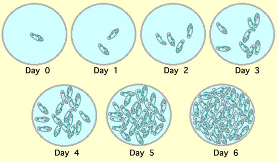
Figure 1: Changes in a population of Paramecium over a six day period
Each individual in the population divides once per day.
The Exponential Equation is a Standard Model Describing the Growth of a Single Population
The easiest way to capture the idea of a growing population is with a single celled organism, such as a bacterium or a cilliate. In Figure 1, a population of Paramecium in a small laboratory depression slide is pictured. In this population the individuals divide once per day. So, starting with a single individual at day 0, we expect, in successive days, 2, 4, 8, 16, 32, and 64 individuals in the population. We can see here that, on any particular day, the number of individuals in the population is simply twice what the number was the day before, so the number today, call it N(today), is equal to twice the number yesterday, call it N(yesterday), which we can write more compactly as N(today) = 2N(yesterday).
Since the basic rule of cell division applies not only to today and yesterday, but to any day at all, we would have N(6) = 2N(5), or N(4) = 2N(3), etc.
So it makes sense to write this as, N(t) = 2N(t - 1) where t could take on any value at all.
Now we can generalize this idea a bit if we note that at day six the number is equal to twice the number at day five, or N(6) = 2N(5) and at day five the number is equal to twice the number at day four, or N(5) = 2N(4), etc.
So in the equation for day 6 we can substitute for the value of N(5) — which we know to be 2N(4) — getting N(6) = 2[2N(4)], which is the same as N(6) = 22N(4).
But N(4) = 2N(3), so we can substitute for N(4) getting N(6) = 22N(4) = 22[2N(3)] = 23N(3). And if we follow the same pattern we see that N(3) = 23N(0), which we can substitute for N(3) to get N(6) = 26N(0). Thus we can see a relatively simple generalization, namely
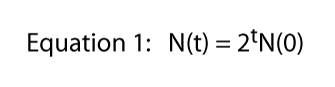
where t stands for any time at all (e.g., if t = 6, N(6) = 26[N(0)]).
Finally we note that this equation was derived from the specific situation shown in Figure 1, where one division per day was the hard and fast rule. That is where the 2 comes from in Equation 1 — from each individual Paramecium we obtain two individuals the next day. Of course the division rate could be anything. If there were two divisions per day but one cell always died, we would expect three individuals from each single individual and Equation 1 would be N(t) = 3tN(0). So the division rate could be any number at all and the general equation becomes,
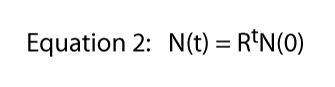
where R is usually called the finite rate of population increase (in the actual case of dividing Paramecium the finite rate of population increase is equal to the division rate). In Figure 2 we illustrate this equation for various values of R. It is normally referred to as the exponential equation, and the form of the data in Figure 2 is the general form called exponential.
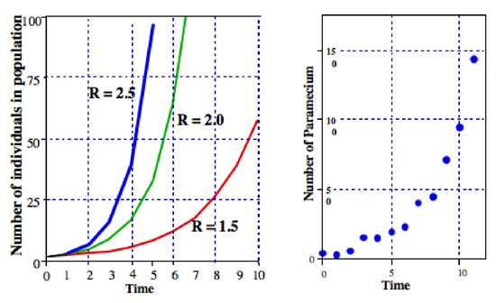
Figure 2: Left: general form of exponential growth of a population (equation 2). Right: actual numbers of Paramecium in a 1 cc sample of a laboratory culture.
Any value of R can be represented in an infinite number of ways (e.g., if R = 16, we could write R = 8 x 2, or R = 42, or R = 32/2, or R = 2.718282.77). That last expression (R = 2.718282.77) makes use of an important constant that might be recalled from elementary calculus, Euler’s constant. Expressing whatever value of R as Euler’s constant raised to some power is actually extremely useful — it brings the full power of calculus into the picture. If we symbolize Euler’s constant as e we can write Equation 2 as
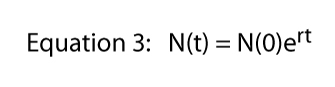
Now if we take the natural log of both sides of Equation 3 — remember ln(ex) = x — Equation 3 becomes: ln [N(t)] = ln [N(0)] + rt
And if we began the population with a single individual (as in the example above), we have

from which we see that the natural log of the population, at any particular time, is some constant, times that time. The constant r is referred to as the intrinsic rate of natural increase (Figure 2).
All sorts of microorganisms exhibit patterns that are very close to exponential population growth. For example, in the right hand graph of Figure 2 is a population of Paramecium growing in a laboratory culture. The pattern of growth is very close to the pattern of the exponential equation.
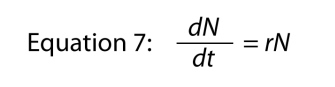
Another way of writing the exponential equation is as a differential equation, that is, representing the growth of the population in its dynamic form. Rather than asking what is the size of the population at time t, we ask, what is the rate at which the population is growing at time t. The rate is symbolized as dN/dt which simply means “change in N relative to change in t,” and if you recall your basic calculus, we can find the rate of growth by differentiating Equation 4, which gives us
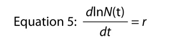
which is kind of remarkable, because it says that the rate of growth of the log of the number in the population is constant. That constant rate of growth of the log of the population is the intrinsic rate of increase.
Recall that the rate of change of the log of a number is the same as the “per capita” change in that number, which means we can write Equation 5 as

where we omit the variable t since it is obvious where it goes, and then we rearrange a bit to come up with
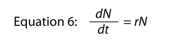
where the parameter r is, again, the intrinsic rate of natural increase. The basic relationship between finite rate of increase and intrinsic rate is
r = ln(R)
where ln refers to the natural logarithm. Note that Equation 6 and Equation 3 are just different forms of the same equation (Equation 3 is the integrated form of Equation 6; Equation 6 is the differentiated form of Equation 3), and both may be referred to simply as the exponential equation.

Figure 3: Hypothetical case of a pest population in an agroecosystem
According to model 1 (which has a relatively large estimate of R), the farmer needs to think about applying a control procedure about half way through the season. According to model 2 (which has a relatively small estimate of R), the farmer need not worry about controlling the pest at all, since its population exceeds the economic threshold only after the harvest. Clearly, it is important to know which model is correct. In this case, according to the available data (blue data points), either model 1 or 2 appears to provide a good fit, leaving the farmer still in limbo.
The exponential equation is also a useful model for developing intuitive ideas about populations. The classic example is a pond with a population of lily pads. If each lily pad reproduces itself (two pads take the place of where one pad had been) each month, and it took, say, three years for the pond to become half filled with lily pads, how much longer will it take for the pond to be completely covered with lily pads? If you don’t stop to think too clearly, it is tempting to say that it will take just as much time, three years, for the second half of the pond to become as filled as the first. The answer, of course, is one month.
Another popular example is the proverbial ancient Egyptian (or sometimes Persian) mathematician who asks payment from the king in the form of grains of wheat (sometimes rice). One grain on the first square of a chess board, two grains on the second square, and so forth, until the last square. The Pharaoh cannot imagine that such a simple payment could amount to much, and so agrees. But he did not fully appreciate exponential growth. Since there are 64 squares on the chess board, we can use Equation 2 to determine how many grains of wheat will be required to pay on the last square (R raised to the 64th power, which is about 18,446,744,074,000,000,000 — a lot of wheat indeed, certainly more than in the whole kingdom). These examples emphasize the frequently surprising way in which an exponential process can lead to very large numbers very rapidly.
The Idea of Density Dependence Modifies the Exponential Equation
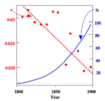
Figure 4: Growth of the human population of the United States of America during the nineteenth century (blue curve), and estimates of the intrinsic rates of increase during that period (red data points)
Note the general tendency for r to decrease throughout the century even while the overall population is increasing.
The idea was originally associated with the human population, and was brought to public attention as early as the eighteenth century by Sir Thomas Malthus. His writings influenced Darwin’s thinking, and formed an important component of the development of the idea of evolution by natural selection. Unfortunately, it is only the more exaggerated claims of Malthus that are normally cited, usually in the context of the growth of the human population. Malthus talked quite a lot about what in fact limits population growth. Indeed, an analysis of the growth of the US human population in the nineteenth century reveals an interesting pattern, one that is repeated with many other organisms. If we estimate the intrinsic rate of increase (the r in Equation 6) for short periods of time during the nineteenth century, we find that there is a general decrease in those estimates during the century, at the same time there is an increase in the numbers in the population (Figure 4).
These data for the US human population suggest something general about populations — as population numbers increase, the estimate of the intrinsic rate of natural increase; over a short period of time, tends to decrease. This means that there is a general relationship between the intrinsic rate of increase and population density. We can plot the data from population studies like the one shown in Figure 4 as a graph of population density versus the estimate of intrinsic rate of increase. The general appearance of such a graph is illustrated in Figure 5, for the same laboratory population of Paramecium that we looked at before. (Figure 5).
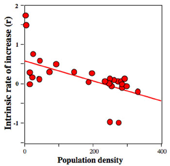
Figure 5: Representing the intrinsic rate of increase as a function of population density for a laboratory population of Paramecium
The higher the population density, the lower the intrinsic rate of increase.
The pattern in Figure 5 is very typical of many populations in both laboratory and natural settings. As with most data from real populations, there is considerable variation. But the trend is clear — with higher population densities, the intrinsic rate of increase tends to be smaller. So, ecologists have made a kind of generalization about this common pattern. The intrinsic rate of increase, as defined in the exponential equation, is not a constant number at all but rather is itself a function of the density of the population. As with many initial attempts at quantifying a concept, we assume a linear approximation (e.g., the straight line drawn through the data points in Figure 5).
If we presume the r of the exponential equation is a function of N (the population density), rather than writing
as we did before (we keep the equation numbering system the same, so this equation is still Equation 3), we must modify it in accordance with the observation that r is a function of N (which we write r = f[N]), which makes Equation 6 turn into
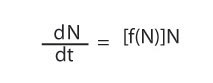
But if we assume f(N) is linear, we must write f(N) = a - bN, where a and b are two constants. So Equation 6 turns into
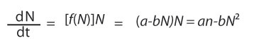
from which you can see that the differential equation of population growth takes on a quadratic form, which means it has a shape that looks sort of exponential when N is very small, at the beginning of a population trajectory, and levels off as N becomes large. The basic form of this equation is shown in Figure 6 when fitted to data from the same laboratory population of Paramecium used to compute the data plotted in Figure 5 (Figure 6).

Figure 6: A laboratory population of Paramecium
Note how the density first looks exponential (indeed these are the same data presented in figure 2, but over a longer time frame), but later, after the population gets to around 300 cells per cc, it levels off. This is the classic logistic pattern.
There is an alternative way of dealing with this same problem, one that usually makes more intuitive sense since it provides the arbitrary constants with biological meaning. Consider the situation in Figure 7. This is a picture of a caterpillar that lives in the tropical rain forests of Central America. The really interesting part of the picture is all the small white cocoons on its back. These are cocoons filled with small parasitic wasps. The adult wasp lays eggs on the caterpillar when it is young and the larval wasps eat the tissue of the growing caterpillar until they reach pupating size, at which time they emerge through the cuticle of the caterpillar’s skin and form a cocoon, as you see in Figure 7. Here we have a situation that would seem to create a natural limit for the population density of the wasps. If you count the cocoons on the caterpillar in Figure 7, you will find there are 80 cocoons on this one hapless caterpillar. Suppose there are 100 caterpillars in the environment. If this caterpillar represents the highest number of wasps that could possibly successfully complete their life cycle on a single caterpillar (most likely the case), we can then say that there is a ceiling on the potential population density of the wasps of 100 x 80 = 8000. Thus this environment for this species of wasp has a carrying capacity of 8000 (Figure 7).

Figure 7: Tropical American caterpillar with parasitic wasps emerging and forming cocoons on the caterpillar's back
Courtesy of John Vandermeer.
Now we go back to the exponential equation and ask what needs to be changed about it to take into account of this kind of population ceiling, the carrying capacity. As before we can speculate that what happens in a population is that its effective intrinsic rate of increase actually changes as the density of the population changes. But now we have a new biological concept we can use in developing this theory — the carrying capacity. Let us suppose that the rate at which a population is increasing at any given point in time is proportional to the relative amount of space available to the population — a population with very few individuals will have a lot of space left and will thus grow rapidly, whereas a population with many individuals will have less space left and will thus grow more slowly. That is, to take the concrete example of the parasitic wasps in Figure 7, if there are 100 caterpillars in the environment, and there is space for 80 wasps at the most in each of them, then there is space for 8000 wasps in this environment. The actual amount of space that remains available to the wasp population is 8000 - N, where N is the current population density of wasps. Thus the relative amount of space left will be (8000 - N)/8000 (divide by 8000 because we wish to calculate the relative amount of space left — the proportion or percentage of what could be maximally available). Population ecologists usually use the symbol K for the carrying capacity, so the intrinsic rate would be multiplied by (K - N)/K. Substituting this Figure for the f(N) (which is the function that the intrinsic rate of increase is) gives us our final result, the famous logistic equation that describes logistic population growth.
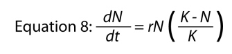
Its basic form has already been introduced (see Figure 6), and note that with a little bit of algebra the arbitrary constants, a and b of Equation 7, take on intuitive biological meaning (i.e., a = r and b = r/K). For many smaller organisms such as bacteria, ciliates, various amoeboid organisms, diatoms, and others, this equation describes population growth reasonably well. For larger organisms such as elephants, humans, trees, or even mice, it is usually thought to be too simple. More complicated models have been developed that take into account more aspects of an organism’s life, but these are beyond the scope of an elementary introduction. For now, all that is necessary to know is that much of population ecology, population genetics, and related fields have, as part of their founding rules, the exponential equation and the logistic equation.