


« Prev Next »

Community ecology is the study of a set of species co-occurring at a given time and place. A central aim of community ecology is to understand how communities are organized by identifying, describing, and explaining general patterns that underlie the structure of communities. An example of such a pattern is that some species never occur together in the same place. Such a pattern may be explained in various ways: one species may exclude the other through competition or, alternatively, they simply prefer different habitats.
Although it may be relatively easy to explain patterns when only a handful of species are involved, it has proven difficult to provide general rules about entire communities where many species co-occur and interact. Such general rules would be very useful as they increase our understanding of how communities function and allow predictions as to how they would respond to environmental changes, for example global warming or restoration efforts. Although there are few rules that are universally true in community ecology (Lawton 1999), there are regular, predictable patterns. Within most natural assemblages a few species comprise the majority of the individuals (Figure 1; Preston 1948). This pattern in distribution of species abundances is accompanied on a larger scale level, by the tendency of widespread species to also occur in higher densities compared to species restricted in their geographic distribution. This relationship is termed the distribution-abundance relationship.

Figure 1: The commonness and rarity of species in a community
In nearly every community in which species have been identified and counted, distributions are highly skewed such that a few species are present in the greatest numbers. In a mesotrophic ditch more than half of all the individuals belonged to one species Hygrotus decoratus (A1–A3). Other species of water beetles are Noterus crassicornis (B1–B2), Liopterus haemorrhoidalis (C1), Acilius canaliculatus (B3, C3) and Hydrochus carinatus (C2).
© 2011 Nature Education Photo courtesy of W. C. E. P. Verberk All rights reserved. 
Both patterns are among the most robust patterns in community ecology. Their robustness and consistency across species groups and ecosystems suggests that there are general macroecological rules underlying the abundance and distribution of species. In the remainder of this article, I discuss each one in more detail.
Patterns in Species Abundance
Knowing the abundance of different species can provide insight into how a community functions. Data on species abundances are relatively easy to obtain, and may give insight into less visible aspects of a community, such as competition and predation. For example, observations that two species occur together in many places, yet never co-occur at high densities (i.e., when one species is numerous, the other is scarce), suggests that these species compete with each other. Comparing species abundance among communities can be difficult because communities often comprise many different species whose abundance profiles differ widely among the communities. Species abundance curves, in which the number of species is plotted against their abundance, are used to deal with this complexity. By condensing the information on species abundances, they allow for comparisons of how various communities differ in the way they are organized. Contrasting patterns in species abundance may similarly indicate differences in the way that communities are organized. For example, the periodic intrusion of seawater into salt marshes (Figure 2A) may constitute a disturbance that prevents most species from becoming abundant other than a few species that are able to cope with the periodic exposure to salt water. As a result, there is a large disparity in the abundance of species from the species-poor communities found in salt marshes (Figure 2C). The rich structural complexity in fen wetlands (Figure 2B) may lead to a fine partitioning of available habitat space. As a result, the pattern in species abundance may be more uniform; for the many species that co-occur in fen wetlands, differences in their abundance are much more gradual, sometimes also referred to as being more evenly distributed (Figure 2D).

Figure 2: Differences between communities in equitability of abundances
(A) Communities in salt marshes are species poor and characterized by a very skewed pattern in species abundance, possibly owing to periodic disturbance by seawater. (B) In contrast, structurally complex fen systems are species rich and have a more even community abundance pattern, possibly owing to a fine partitioning of available niches. Hypothetical species abundance distributions illustrate the differences in species abundance distribution between (C) the salt marsh where 15 species show quite unequal abundances and (D) the fen system where the same number of individuals is distributed more equally over twice as many species.
© 2011 Nature Education Photos courtesy of W. C. E. P. Verberk All rights reserved.
In nearly every community in which species have been identified and counted, distributions are highly skewed. That is, there are many rare species and only a few common species. Although a skewed pattern in species abundance seems to be a universal feature of all communities, it may be more pronounced in some ecosystems, such as salt marshes (Figure 2A, C), and less pronounced in other ecosystems, such as fens (Figure 2B, D). To determine what "more" and "less" actually mean, we need to quantify the degree to which such patterns are skewed. One way to deal with skewed abundances is to transform them using logarithms. This is visualized by Preston's log-normal distribution of species abundance (Preston 1948). He constructed abundance intervals, each interval being twice the preceding one and graphed the number of species within each interval (Figure 3). When plotted on this log 2 scale, patterns in abundance were found to approach a normal distribution (hence the name log-normal distribution). For many communities a log-normal distribution provides an accurate description of the abundances of species in a community, and this distribution is therefore frequently used to model the relative abundance of species in communities. Besides the log-normal distribution, there are other mathematical models (e.g., geometric series, log series, broken stick) in use, each incorporating different mathematical assumptions and theoretical concepts of how communities function (McGill et al. 2007).
Using logarithms to transform data is simply another way of plotting abundance data that facilitates comparisons of the data across communities. However, assuming that abundances in natural communities are indeed log-normally distributed has some practical consequences. According to a log-normal distribution, not only are there few common species with a high local abundance, but also few species seem to be truly rare. This makes sense intuitively, as species with small populations are more likely to go extinct. Hence the number of species with small populations should be limited. Yet this prediction is not always borne out by field data; indeed, most species in a sample are rare. One reason may be that it requires extensive sampling before the log-normal distribution becomes evident. Incomplete sampling will often miss some species. Preston noted that more intensive sampling will "unveil" these species (i.e., shift the ‘veil line' in Figure 3 to the left). Deviations from a log-normal distribution, therefore, can be used to estimate the completeness of a species inventory and estimate how many more species might be found if sampling is more intensive. As community sampling is always incomplete, this information has significant practical value. Being able to extrapolate information from a limited number of samples improves the effectiveness of species inventories, including monitoring changes in species abundances due to global warming or restoration efforts, for example.

Figure 3: Species abundance distributions on a log-normal scale
The number of species plotted for different abundance intervals, each interval being twice the preceding one. The portion of the graph (red) left of Preston's veil line is theoretical, depicting those species that are expected to be present but their low abundance prevents them from being represented in the sample.
© 2011 Nature Education All rights reserved.
Distribution-abundance Relationship
Species that are restricted in their geographic distribution tend to be scarce whereas widespread species are likely to occur at high densities. This positive interspecific distribution-abundance relationship (Figure 4A) is intimately related to the patterns in species abundance discussed earlier. This relationship may seem self-evident: Surely there is a positive link between measures of a species' success on a local scale (its density) and on a regional scale (its geographic distribution). Yet although a larger area is more likely to be able to sustain a higher total number of individuals of a species, it is not clear why the density (number of individuals in a given area) should also increase.
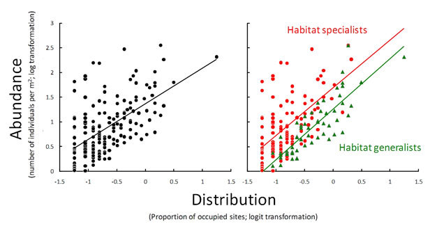
Figure 4: The interspecific distribution-abundance relationship
(A) Generally, a positive relationship results when plotting measures of abundance against measures of distribution for different species from a species group. (B) The same data, with species subdivided into habitat specialists (red) and habitat generalists (green), showing that habitat specialists may be more abundant relatively (i.e., for a given distribution). A logit transformation is given by logit (X) = log (X/1-XM).
© 2011 Nature Education Data from Verberk, W. C. E. P. et al. (2010) All rights reserved.
It is vital to understand how the processes linking the local abundance of a species and its regional distribution because this has some far reaching consequences. For example, suppose that restricted ranges inevitably lead to low densities. Then efforts to conserve a particular species by protecting a small part of high quality habitat will not be effective. Similarly, control of invasive species can be most fruitfully directed to prevent range expansion. If on the other hand, high local densities inevitably lead to range expansion, then the conservation efforts outlined above may be very effective, while control of invasive species is best achieved by local eradication efforts.
There are two broad classes of ecologically based explanations for interspecific distribution-abundance relationships. The first class postulates the existence of a positive feedback between local abundance and the regional distribution of a species (Figure 5A). Species that occur in large numbers across many localities will be more likely to maintain their wide distributions and high abundance. Larger populations produce more offspring, which increases the chances that the species will reach other localities (higher colonization) and expand its geographic range. Similarly, being widespread will ensure the continuous arrival of individuals to all places and thus a species will be less likely to disappear from a particular locality (lower local extinction). A consequence of this positive feedback is that there is a dichotomy: Species will either be widespread and abundant (so called core species) or they will be restricted and scarce (so called satellite species).

Figure 5: Explanations for a positive distribution-abundance relationship
(A) A positive feedback between local population size and regional distribution may generate a positive distribution-abundance relationship. (B) Spatially autocorrelated differences in habitat quality and the way they are experienced by different species generates a positive relationship between the abundance and distribution of species.
© 2011 Nature Education All rights reserved.
The second class focuses on niche differences among species. Both physical (temperature, rainfall) and biotic (predators, competitors) factors may limit the survival and reproduction of a species, and hence its local density and geographic distribution. The combination of these factors, and the point at which they limit a species' survival and reproduction, constitutes the multidimensional niche of a species (Hutchinson 1957). The density that a given species can attain at a certain locality is assumed to also reflect its tolerance to the environmental conditions prevailing at that locality. Localities are likely to be more similar if they are in close proximity because of spatial autocorrelation (i.e., the similarity in environmental conditions between localities is inversely related to the distance between them). Hence locally abundant species will also be able to occupy localities across a larger geographic range (Figure 5B). A distinction is made between species with a broad niche (generalists) and species with a narrow niche (specialists). Generalists are able to tolerate a broad set of environmental conditions and use a wide range of resources, enabling them to become both widespread and locally abundant; in other words, the jack-of-all-trades is the master of all (Brown 1984).
A relevant question is whether geographical distribution and local abundance both contribute to extinction risk. More specifically, if specialist and satellite species face a double jeopardy of extinction (i.e., they are prone to extinction due to their low abundance and restricted distribution), this raises the question why there are so many species within these categories (see patterns in abundance discussed above)? Although measuring a species' niche breadth is not a simple task given the large number of potentially relevant factors that may limit the survival and reproduction of a species, there is currently little evidence that generalists are more abundant than specialists. Indeed, specialists may even be more abundant than generalists after accounting for their narrow distribution (Figure 4B). Thus specialists may persist through numerically larger local populations. This suggests that the jack-of-all-trades (i.e., generalists having a broad geographic distribution) could in fact be the master of none (Verberk et al. 2010).
Explaining Both Macroecological Patterns: Two Opposite Approaches
The patterns in species abundance and geographic distribution discussed above have been explained in various ways. The various explanations differ in the assumptions and operational mechanisms, yet they all provide an explanation for the (same, near universal) patterns of a skewed pattern in species abundances or a positive distribution-abundance relationship. As the same pattern can arise in different ways, a more detailed description of the shape and form of these patterns in species abundance and geographic distribution is unlikely to tell us which explanation is most valid in a given situation. However, the validity of the assumptions, and the operation of the mechanisms, can be tested with empirical data. To illustrate the main points, this discussion is limited to explanations encompassing either niche dynamics or neutral dynamics.
Niche dynamics assumes that there are differences among species in their multidimensional niches that should give rise to patterns in the abundance and distribution of each species. A grassland experiment demonstrated such differences among species of plants (Harpole & Tilman 2007). Plants compete for various soil resources (e.g., phosphorous and nitrogen) essential for plant growth. Niche differences can facilitate species coexistence when, for example, one species is better able to tolerate low levels of phosphorus (thus that species can outcompete other species, but only under conditions of limited phosphorous) while another species is tolerant of low nitrogen levels (a superior competitor when nitrogen is limited). Plant numbers were shown to decrease when the experimenter added nutrients so that they were no longer limiting. Species could no longer partition the available space according to their specific niche requirements as the nutrient addition removed any spatial distribution where one or the other of these (previously limiting) resources was limiting, reducing the opportunities for coexistence among species. This demonstrates that species do indeed differ in their multidimensional niche; the point at which various resources become limiting for survival and reproduction varies among species.
According to niche dynamics, the abundance and distribution of a single species, and hence the emergent patterns across multiple species, are driven by causal mechanisms operating at the level of that species. Therefore, examining the effect of differences among species (for example differences in their dispersal capacity or ability to tolerate harsh conditions) on patterns in their abundance and geographic distribution may demonstrate the importance of those differences. For example, Magurran and Hendriks (2003) found that samples of a given community contain a mixture of both species from elsewhere and species which are biologically associated with that community. Species dispersing from elsewhere inflated the number of rare species, and the abundances of these immigrants did not follow a log-normal distribution, in contrast to the resident species associated with the community. Similarly, Sugihara et al. (2003) demonstrated a relationship between niche similarity among species and their abundance patterns. Communities in which differences among species' niches were more gradual or evenly distributed also had less skewed abundance patterns (e.g., Figure 2D), whereas communities with unevenly distributed niche differences among species had more skewed abundance patterns (e.g., Figure 2C). For distribution-abundance relationships, there is evidence that distribution-abundance relationships are driven by causal mechanisms operating at the level of that species (Verberk et al. 2010). Specific information on a species' diet, reproduction, dispersal, and habitat specialisation could explain most of a species' contribution to the overall distribution-abundance relationship.
Neutral dynamics assumes that species and habitats are equivalent, and patterns in species abundance and distribution arise from stochastic occurrences of birth, death, immigration, extinction, and speciation (Hubbel 1997). Different probabilities associated with these stochastic occurrences can be entered into a computer program to simulate communities. Such simulated communities constitute a null model: how much of the patterns seen in nature may be due to pure chance? Somewhat surprisingly, the simulated communities exhibited patterns in species abundance and distribution which were strikingly similar to those in nature, including Preston's log-normal distribution and a positive distribution-abundance relationship. One could thus infer that niche differences among species are unimportant. However, accurately modeling real-life patterns does not necessarily mean that the model's assumptions reflect the actual mechanisms underlying these real-life patterns. In fact, patterns in species' abundance and distribution-abundance relationships are generated across many species, without taking into account the identity of a species. Therefore, it may not be surprising that neutral models can accurately describe these community properties.
As so often occurs in ecology, different explanations are not always mutually exclusive. In dynamic environments with pronounced environmental gradients (e.g., communities of invertebrates in intertidal rocky shores), niche differences are likely to play an important role. In contrast, neutral dynamics may be the dominant force in less variable environments such as a community of tropical forest trees, where dispersal limitation and a long lifespan may prevent competitive exclusion. Neutral dynamics may be relatively important in some cases, depending on the species, environmental conditions and the spatial and temporal scale under consideration, whereas in other circumstances, niche dynamics may dominate. Thus niche and neutral dynamics may be operating simultaneously, constituting different endpoints of the same continuum.
Summary
I have discussed two of the most robust patterns in community ecology: (1) the skewed pattern in species abundance, in which a community contains many rare species and only a few common species and (2) the positive distribution-abundance relationship, in which widespread species tend also to occur in high abundance throughout their range. Understanding these patterns has important implications for practical issues like reserve selection and predicting extinction risk. Two independent approaches seek to explain these emergent patterns. The first focuses on neutral dynamics with patterns in species abundance and distribution arising from stochastic occurrences of birth, death, immigration, extinction, and speciation. The second focuses on niche differences among species as the driving force behind the abundance and distribution of a single species, and hence the emergent patterns across multiple species. Both may be operating simultaneously, constituting different endpoints of the same continuum.
Glossary
Abundant: a species is said to be abundant when it is locally numerous or occurs in high densities.
Community: an assemblage of two or more interacting populations of different species occupying the same geographical area at a given time.
Community ecology: the study of the organization and functioning of communities.
Dispersal limitation: the situation where a species' dispersal capacity is insufficient to reach all suitable localities. As a result some localities are not occupied despite their suitability.
Distribution-abundance relationship: the relationship between the local abundance of species and the size of their ranges within a region.
Generalists: species that is able to tolerate a broad set of environmental conditions and use a wide range of resources.
Localities: a specific location in space.
Macroecology: the study of relationships between organisms and their environment at large spatial scales to characterize and explain patterns in species abundance, distribution and diversity.
Multidimensional niche: a multidimensional composite in which all of the boundaries of tolerance of diverse environmental influences are assembled into a single, multivariate factor. This is also known as a hypervolume of environmental tolerance, in which an individual can potentially survive or in which a species can maintain viable populations.
Neutral dynamics: changes in the abundance and or distribution of a species as a result of stochastic occurrences of birth, death, immigration, extinction and speciation.
Niche breadth: the range of environmental conditions a species can tolerate (when related to habitat breadth) or the range of resources a species can utilize (when related to diet breadth). Measuring and calculating niche breadth usually involves measuring abundance of species in various categories of habitat and relating the proportion of a species' population found in each category to the proportion of sampling effort (area sampled) for that category. A species with a narrow niche has specialized exclusively on one category and consequently bypasses all other categories.
Niche dynamics: changes in the abundance and or distribution of a species as a result of species performance (e.g., survival, reproductive success), which is a function of how well a species capabilities match to the prevailing habitat conditions.
Normal distribution: a continuous probability density function where multiple values or measurements are symmetrically distributed around a single mean value, giving rise to bell-shaped density curves with a single peak. The graph of the associated probability density function is also known as the Gaussian function or bell curve.
Patterns: regularities in the organization of communities as evidenced by consistent recurring observations.
Reserve selection: the process of selecting sites to be included in nature reserve networks to safeguard the biodiversity contained within these sites. Sites can be selected according to various criteria (e.g., in the short term, the contribution in terms of natural values compared to already protected sites may be important, while in the long term it may be important to also take into account climatic projections).
Restricted: a species is said to be restricted when it can only be found in a small geographic area; it has a small geographic range.
Scarce: a species is said to be scarce when it is not locally numerous or occurs in low densities.
Specialists: a species that is able to tolerate a narrow set of environmental conditions and use a narrow range of resources.
Species abundance distribution (SAD): a description of the commonness and rarity of species in a community by means of a frequency distribution of species abundances.
Widespread: a species is said to be widespread when it can be found across a large geographic area; it has a large geographic range.
References and Recommended Reading
Brown, J. H. On the relationship between abundance and distribution of species. The American Naturalist 124, 255–279 (1984).
Harpole, W. S. & Tilman, D. Grassland species loss resulting from reduced niche dimension. Nature 446, 791–793 (2007).
Hubbell, S. P. A unified theory of biogeography and relative species abundance and its application to tropical rain forests and coral reefs. Coral Reefs 16 (Suppl.), S9–S21 (1997).
Hutchinson, G. E. Concluding remarks. Cold Spring Harbor Symposium. Quantitative Biology 22, 415–427 (1957).
Lawton, J. H. Are there general laws in ecology? Oikos 84, 177–192 (1999).
Magurran, A. E. & Hendriks, P. A. Explaining the excess of rare species in natural species abundance distributions. Nature 422, 714–716 (2003).
McGill, B. J. et al. Species abundance distributions: Moving beyond single prediction theories to integration within an ecological framework. Ecology Letters 10, 995–1015 (2007).
Preston, F. W. The commonness, and rarity, of species. Ecology 29, 254–283 (1948).
Sugihara, G. et al. Predicted correspondence between species abundances and dendrograms of niche similarities. Proceedings of the National Academy of Sciences of the United States of America 100, 5246–5251 (2003).
Verberk, W. C. E. P., van der Velde, G. & Esselink, H. Explaining abundance-occupancy relationships in specialists and generalists: A case study on aquatic macroinvertebrates in standing waters. Journal of Animal Ecology 79, 589–601 (2010).