How individuals are arranged in space can tell you a great deal about their ecology. For instance, Figure 1 shows the distribution of a hypothetical species. Most people would describe this as a random pattern in space. However, if you look closely you will notice that individuals are not actually randomly distributed, they are maintaining a fairly uniform distance between each other. Why do you think that is? Figure 2 shows the distribution of another hypothetical species. This time they are grouped together in certain 5 x 5 meter areas but not in others. What might this tell you about this species and its interactions with the environment? Figure 3 shows the distribution of individuals of a hypothetical species that is actually random. One thing that you'll notice is that it is difficult to think of this as random!

Figure 1: Clumped dispersion of individuals

The average number of individuals per square is 6.25, the variance is 125, and the ratio of the two is 20.

© 2011 Nature Education All rights reserved.

These three figures illustrate the three different patterns of dispersion that ecologists observe. Clumped dispersion (Figure 1) where individuals are aggregated in certain areas of the sampled space. Uniform dispersion (Figure 2), where individuals are almost equally spaced apart from each other and random dispersion (Figure 3).

Figure 2: Uniform dispersion of individuals

The average number of individuals per square is 10, and the variance is 4.27. The variance to mean ratio is 0.427.

© 2011 Nature Education All rights reserved.

Behavioral and ecological factors influence dispersion. Uniform patterns of dispersion are generally a result of interactions between individuals like competition and territoriality. Clumped patterns usually occur when resources are concentrated in small areas within a larger habitat or because of individuals forming social groups. At large spatial scales most organisms appear to have clumped distributions because their habitats are not uniformly distributed over wide areas. Although you might not think of plants as territorial, they too can have uniform dispersion patterns that are a result of territoriality and competition (e.g., shading, allelopathy, and root interactions; Mahall & Callaway 1992, Schenk et al. 1999). Random dispersion patterns are atypical in nature and could indicate a uniform or random distribution of resources or a lack of interactions among individuals in the population.

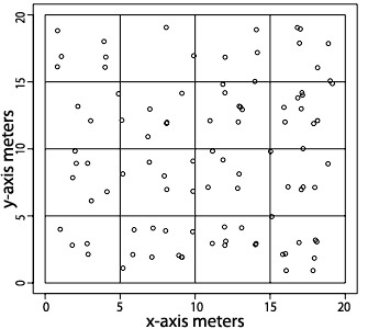
Figure 3: Random dispersion of individuals

The mean number of individuals per square is 5.94, the variance is 5, and the ratio is 0.841.

© 2011 Nature Education All rights reserved.

Humans are not always very good at distinguishing among the different patterns of dispersion, so statistical methods are usually used to tell the difference between them.

A very simple method that can be used to determine dispersion patterns is based on the sample mean and variance of the number of individuals counted in repeated quadrats in a particular area that is sampled. The sample mean is the average collected from the sample. As an example, let's examine Figure 1. This figure is divided into squares, and each square represents a sample of organisms in space. In this case the organisms are clumped in space and there are 4 samples with 25 organisms and 12 with no organisms. The sample mean is calculated as the sum of all of the observations (25 + 25 + 25 + 25 + 0 + 0 + 0 + 0 + 0 + 0 + 0 + 0 + 0 + 0 + 0 + 0) divided by the total number of samples (16). Thus the mean number per square in Figure 1 is 6.25. The variance is calculated by squaring the differences between the sample mean and each of the observations, adding them up to produce the sum of the squares, and dividing by the sample size minus 1. So the variance in this case would be ([25 - 6.25]² + [25 - 6.25]² + [25 - 6.25]² + [25-6.25]² + [0 - 6.25]² + [0 - 6.25]² + [0 - 6.25]² + [0 - 6.25]² + [0 - 6.25]² + [0 - 6.25]² + [0-6.25]² + [0 - 6.25]² + [0 - 6.25]² + [0 - 6.25]² + [0 - 6.25]²)/(16 - 1) which is 125. So in Figure 1 the average number of individuals per grid square is 6.25 and the variance among grid squares is 125. The ratio of the variance to the mean can then be used to determine whether the pattern is uniform or clumped, and is referred to as the index of dispersion (Krebs 1999). In this case the ratio is 20, which is much greater than 1! This indicates that individuals in this population are exhibiting a clumped spacing pattern in the sampled habitat. If this ratio is less than one, it indicates a uniform distribution (e.g., Figure 2, ratio = 0.427). Whereas if it is one, that indicates individuals are randomly distributed in space (e.g., Figure 3, ratio = 0.841). While this method is extraordinarily simple and widely illustrated in many texts, it can potentially fail to detect some non-random patterns of dispersion (see Krebs 1999).

The distances between individuals can also be used to determine dispersion patterns. Several indices exist, but all operate using similar principles. If individuals are aggregated or clumped (Figure 2), their nearest neighbor will be much closer than you would expect if individuals were randomly distributed in space (Figure 3). If they were uniformly distributed (Figure 1), on average, you would predict individuals to be further apart than would be expected if they were randomly distributed.

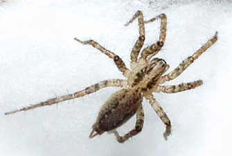Figure 4: Agelenopsis sp. on a sheet web

© Creative Commons Patrick0Moran via Wikimedia Commons Some rights reserved.

Explaining these patterns requires investigation of the availability of suitable habitat as well as the interactions among individuals. At a larger spatial scale a very small amount of the habitat is suitable for websites and, of course, that is where the spiders are (Riechert 1981). These spiders prefer large depressions in grassland habitats with characteristics attractive to insect prey (e.g., flowering shrubs, the presence of litter, and animal feces) and have favorable thermal properties (Reichert & Gillespie 1986). The spatial distribution of these suitable habitats is what generates the clumped pattern at a larger scale. Since high quality websites are limited in the habitat, and the presence of other spiders in close proximity reduces the fitness of the resident spider, residents will actively patrol their website and engage in aggressive behavior towards other spiders enter into their territory (Riechert 1981). These interactions generate a minimum spacing among individuals within suitable habitat patches, and the occasional displacement of individuals from their website (Riechert 1981, Riechert & Gillespie 1986). Aggressive interactions like these are typical of the types of behavioral interactions that generate uniform spacing patterns.