


« Prev Next »
What is an alternative stable state?
The current condition of an ecological system is its state. Because , it is possible for them to occupy more than one state for a given set of environmental conditions. In other words, while a system may have the Which alternative state is occupied depends on the history of the system and the perturbations to which it has been exposed. Alternative states are stable when they are maintained following further small perturbations. In the following article we will learn more about alternative stable states in ecology and develop a simple model that reveals how important related concepts are defined.
Purported examples of alternative stable states (ASS)
There are many observed examples that infer the presence of ASS (see Beisner et al. 2003b, Folke et al. 2004 and Knowlton 2004 for reviews), including the collapse of fisheries owing to food web interactions and harvesting (Steele 1998, Jackson et al. 2001) and the shift from healthy coral reef communities to macroalgae (Hughes 1994) in marine environments. In the Serengeti, there are shifts between woodlands and herbaceous plants regulated by elephant activity and their pests (Dublin et al. 1990). Another commonly studied example is a shift between clear and turbid water states in ponds and lakes (e.g. Scheffer 1993, Beisner et al. 2003a). There are fewer examples from experimentally-induced ASS (but see Van de Koppel et al. 2001, Petraitis and Dudgeon 2004, Schröder et al. 2005) and one reason may be because the scale at which disturbances must occur are often too large for experimentation (Petraitis and Latham 1999). ASS are not restricted to ecological systems however; rather they are a generic feature of dynamical systems. Thus we can also find examples from the collapse of societies (Diamond 2005), in the tendencies of stock markets, as well as crime and disease epidemics (Gladwell 2000) among others.
Why do we need to understand ASS?
The fact that ASS can exist is important for a number of reasons. Ecologists are interested in observing and understanding their study systems so as to be able to predict what they might do in the future. The problem with ASS is that if we do not know that they are possible, they present surprises. Thus, our ecological frameworks need to include them, where they may occur, to predict when and why a sudden change might happen. Just knowing the habitat conditions is not good enough if it is possible that two states might persist there. We also need to know if a state change will be easily reversed or not, and how this might best be done if the outcome is an undesirable one. Ecologists must therefore understand the dynamics of their systems to avoid surprising catastrophic changes that are difficult to reverse. To understand dynamics, we need a good theoretical framework, best accomplished with a mathematical model. We will now explore how one might build such theoretical understanding by using a simple example. Through this modelling example we will be able to clearly see how important related concepts to the study of ASS, like resilience and hysteresis, are defined and fit together. Also the catastrophic potential for mistakes that can arise from managing an ecological system as if ASS weren't present become evident through a modelling framework.
Modelling alternative stable states: A simple example
(i) The model:
One of the earliest frameworks for ASS was developed by Noy-Meir (1975) for grazing animals on pasture land. In the model, vegetation grows based on resource availability, but the density of herbivores is controlled by human managers who decide how many grazers to allow on a patch of land. The dynamics of the vegetation (V) through time (t) can be written generally as:
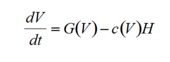
where G(V) is a function defining vegetation growth and c(V) is a function describing the consumption of vegetation by herbivores (H).
A graphical approach provides the simplest glimpse into the dynamics of the system (Fig. 1). The vegetation population grows (G(V)) logistically, with high growth rates when plant biomass is low and resources are abundant, but then declining at higher biomasses as competition for limited resources increases (Figure 1a). Vegetation is consumed (c(V)) by the herbivore according to a Holling Type III functional response (Fig. 1b). The total amount of vegetation removed depends on the stocking density of the herbivores (H), as set by the human managers of the pastureland.
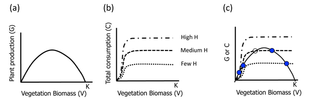
Figure 1
(a) Plant growth (logistic) as a function of plant biomass, where K represents the environmental carrying capacity; (b) herbivore consumption of plant biomass as a function of plant biomass showing a type III functional response whereby herbivory initially increases and then levels off as herbivores become saturated. Three levels of herbivory are shown, as established by stocking densities; and (c) joint plots of plant growth and herbivory. Filled dots (L and U) represent stable equilibria while the empty dot (M) represents an unstable equilibrium point. The letters L,M and H refer to Low, Medium and High vegetation biomass equilibria respectively.
© 2012 Nature Education All rights reserved. 
(ii) Defining the "states":
Now we can ask, what is the state (i.e. equilibrium biomass or V*) of the vegetation in the pasture? And how does this state vary with the number of herbivores stocked. Equilibria occur when the vegetation biomass is no longer changing, thus when dV/dt = 0. Following through algebraically for Eq.1, that means G(V) = c(V)H; and graphically, that the equilibria occur at the intersection of our two sets of lines (Figures 1a and 1b), when plotted together (Figure 1c).
(iii) Stability of "states":
We can now examine the dynamics around each of the equilibria (states) in Figure 1c by asking what happens if we change V very slightly from V* for different levels of herbivore stocking. V will simply return to V* in cases when there are many or few H (top two panels). Graphically, this is because moving the dot to the right along the G line results in more herbivory than plant growth (c line > G line). Likewise, a slight decrease in V (moving dot to the left along the G line) leads to greater plant growth than herbivory (G line > c line). Thus the system always returns to the original equilibrium point. These states or equilibria are therefore called stable.
However in the case of moderate herbivory (Figure 1c; bottom panel), a different situation occurs. Note that there are three equilibrium points now (two filled and one empty dot; Figure 1c). While the two extreme ones (U and L) are stable (as in the cases discussed already), the middle one (M) is unstable. For the middle equilibrium point, a slight increase in V leads to dominance of plant growth (G line > c line) and a continued shift to the right as plants will grow, until they reach the upper equilibrium point (U). A slight decrease in V leads to greater herbivory (c line > G line) and thus further reduction in V* to the lower stable equilibrium (L). For this intermediate herbivore stocking density therefore, we have an example of ASS: there is a low V* (L) and a high V* (U) separated by an unstable equilibrium (M).
(iv) Generating S-curves:
Another way of examining the dynamics of equilibria is by using phase space to plot all possible equilibria in a graph of V vs. H. Understanding such plots is important to interpreting ASS, as one of their common defining features is a phase space plot with a characteristic S-curve (Figure 2) (Schröder et al. 2005). Figure 2 shows how an S-curve is generated for our model: take the value of V* (read off the X-axis) for each equilibrium dot in Fig. 2a and plot this on the Y-axis of Fig. 2b at the value of H to which it corresponds. For example, the left-most (blue) point in Figure 2b thus represents the case where V is high and H is low (blue point in Figure 2a). Each equilibrium is thus transcribed to the new figure and then the points are joined together with a (reversed) S-curve to represent all possible equilibria. The lines marked f1 and f2 in Figure 2a represent important herbivore densities (called bifurcation points). Between these two H lines is the region within which alternative states are possible (i.e. three equilibria). Arrows around each equilibrium show the changes in the biomass of V that would result with slight perturbations from V* as discussed in the previous section. Unstable equilibrium points occur along the dotted line in this region.
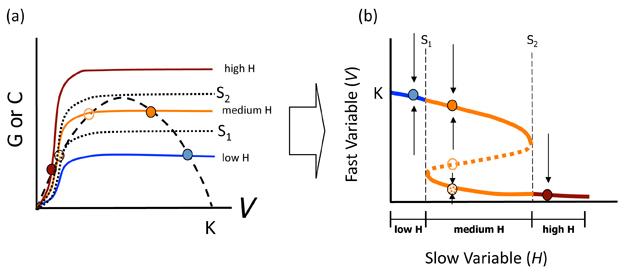
Figure 2
Equilibrium points and lines are similarly coloured in both graphs to show the correspondence. The set of stable equilibria are shown in (b) as solid lines while the set of unstable equilibria are shown as the dashed part of the S-curve. Bifurcation points (f1 and f2) which separate dynamical regions where only one equilibrium point is present from those in which alternative states occur are shown as dotted lines. Arrows in (b) show the dynamics of the system for slight perturbations of V off of the corresponding equilibrium points.
© 2012 Nature Education All rights reserved.
(v) Resilience:
S-curves allow us identify the resilience of the stable states. Resilience is the amount of change or disruption required to transform a system from being maintained by one set of mutually reinforcing processes and structures, to a different set of processes and structures (Peterson et al. 1998). It is an important concept, because it defines how close our system may be to a drastic shift. Returning to our example, for equilibria occurring along the top solid blue line in Figure 2b, all are infinitely resilient as long as H remains low: there will always be high vegetation biomass if there are few herbivores. For equilibria along the lowest end of the S-curve in red, this low V equilibrium is also infinitely resilient as long as herbivores are abundant. It is only for medium H's (orange lines) that resilience changes. Travelling from left to right, equilibria along the top part of the S-curve have decreasing resilience until f2 is reached, at which point resilience of the high V* state is 0. For equilibria occurring along the bottom arm of the orange part of the S-curve, moving again from left to right, resilience increases from 0 at f1. The difference between each solid line and the dotted line defines resilience in each case. Thus, some factor (e.g. a lawn mower, an insect outbreak) that removed more vegetation than that difference for the top solid line would cause a shift to the lower equilibrium line. The opposite case would apply with respect to the resilience of the lower equilibrium line in the face of a "perturbation", such as land managers deciding to plant new vegetation (causing a tip toward the upper equilibrium line). When resilience of either state is low, small stochastic perturbations alone in V* may result in a shift in state even without changing H.
Relevance
Figure 3 shows us why it is important to understand whether such dynamics are possible for the management of an ecological system. If a linear model applies (Figure 3a), there will be no catastrophic surprises when H is changed and a more vegetated state will be easily recovered by simply reversing the last action (i.e. remove one herbivore when there is one too many). This is not the case where alternative states occur (Figure 3b). After flipping to the low V* state, much more work must be done to reverse this action. This contingency represents hysteresis: a condition wherein the reverse path is not the same as the forward path. In our example, we need either to reduce drastically the number of herbivores (H), lower than before we dropped to the depleted V* state (Figure 3b; dotted arrows). Or we need to plant lots of new vegetation to increase V*, after reducing H to a more reasonable number. In either case, going back is not as simple as was going forward. It is the same principle as in "the straw that broke the camel's back". That extra piece of straw turned a once-intact camel into a broken one. One cannot simply remove the piece of straw and have the camel stand up again. One needs to do some more work (surgery?). Thus, managing a complex ecosystem, community or population as if Figure 3a were the case might lead us to some important mistakes that we might avoid were we aware that an ASS was present. Ecological theory and a good understanding of some of the non-linear relationships in our focal system can help ensure we use the right underlying framework to avoid what are often undesirable consequences that are difficult to reverse.
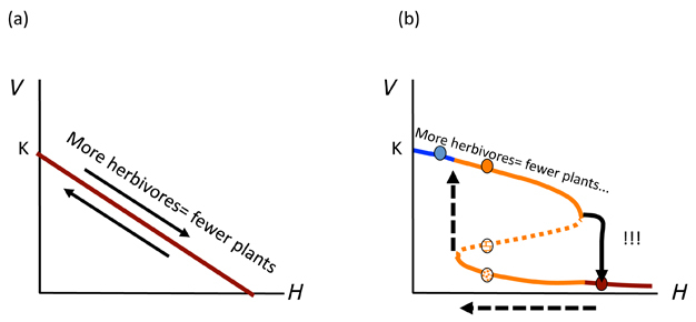
Figure 3
In (a) the incorrect simple linear model is shown whereby additions or removals of herbivores (H) simply move the plant biomass (V*) up or down. In (b) the multiple stable state model discussed in the text is represented whereby increasing H beyond a critical point (bend in the curve) leads to a precipitous decline (!!!) in V*. For the hysteretic system to return to the previously high equilibrium line, H must be reduced to a much lower level (horizontal dashed arrow) before V* will increase (vertical dashed arrow) again.
© 2012 Nature Education All rights reserved.
Glossary
Hysteresis: Observed following a perturbation to an equilibrium point, hysteresis is when the return trajectory to the original equilibrium point or state is different than the outgoing trajectory. In ecological terms, this often means that the "work" that must be done to return to an original state after a disturbance is much more than the "work" done by the original perturbation itself. Hysteresis is a characteristic of alternative stable states and can be used to identify their presence because it means that more than one state can be observed under identical environmental conditions — at least over some range of conditions.
Resilience: The amount of change or size of perturbation required to transform a system from being maintained by one set of mutually reinforcing processes and structures (i.e. one stable ecological state), to a different set of processes and structures (i.e. another stable ecological state) (Peterson et al. 1998). It represents the resistance to change of a particular ecological state.
Stable equilibrium (state): In ecological studies the state can be defined by the set of biotic and abiotic conditions observed for a focal ecosystem or component thereof. When the state is stable, these processes and structures are mutually reinforcing.
References and Recommended Reading
Beisner, B. E., Dent, L. M. & Carpenter, S. R. Variability of lakes on the landscape: Roles of phosphorus, food webs and dissolved organic carbon. Ecology 84,1563-1575 (2003a).
Beisner, B.E., D. Haydon, K.L. Cuddington. Alternative Stable States in Ecology. Frontiers in Ecology and the Environment 1, 376-382 (2003b).
Diamond, J. M. Collapse. New York, USA: Viking Press (2005).
Dublin, H. T., Sinclair, A. R., McGlade, J. Elephants and Fire as causes of multiple stable states in the Serengeti-Mara woodlands. Journal of Animal Ecology 59, 1147-1164 (1990).
Folke, C., Carpenter, S. R., Walker, B., Scheffer, M., Elmqvist, M. T., Gunderson, L., Holling C. S. Regime Shifts, Resilience, and Biodiversity in Ecosystem Management. Annual Review of Ecology, Evolution, and Systematics 35, 557-581(2004).
Gladwell, M. The Tipping Point., Boston, USA: Little, Brown (2000).
Hughes, T. P. Catastrophes, phase shifts, and large-scale degradation of a Caribbean coral reef. Science 265,1547-1551 (1994).
Jackson J. B. C., Kirby M. X., Berger W. H., Bjorndal K. A., Botsford L. W., & 14 more Historical overfishing and the recent collapse of coastal ecosystems. Science 293, 629-638 (2001).
Knowlton, N. Multiple "stable" states and the conservation of marine ecosystems. Progress in Oceanography 60, 387-396 (2004).
Noy-Meir, I. Stability of Grazing Systems: An Application of Predator-Prey Graphs. Journal of Ecology 63, 459-481 (1975).
Petraitis, P.S., Dudgeon, S. R. Detection of alternative stable states in marine communities. Journal of Experimental Marine Biology and Ecology 300, 343-372 (2004).
Petraitis, P. S., Latham, R. E. The importance of scale in testing the origins of alternative community states. Ecology 80, 429-442 (1999).
Scheffer, M., Hosper, S. H., Meijer, M. L., Moss, B. Alternative equilibria in shallow lakes. Trends in Ecology and Evolution 8, 275-279 (1993)
Schröder, A., Persson, L., De Roos, A. M. Direct experimental evidence for alternative stable states: A review. Oikos 110, 3-19 (2005).
Steele J.H. Regime shifts in marine ecosystems. Ecological Applications 8, S33-S36 (1998).
Van De Koppel, J., Herman, P. M. J., Thoolen, P., Heip, C. H. R. Do alternate stable states occur in natural ecosystems? Evidence from a tidal flat. Ecology 82, 3449-3461 (2001).