


« Prev Next »
What is Aging?
Aging is a progressive decline in physiological function, leading to an age-dependent decrease in rates of survival and reproduction (Rose 1991). At the individual level, physiological condition at a particular age determines whether an individual lives or dies and how successful that individual is in reproducing. At the population level, age-specific rates of survival and reproduction summarize the underlying physiological states of the individuals in a population. Demographically, aging is diagnosed if we observe an age-specific decrease in survival in the population; from such a pattern we infer that age-progressive physiological degeneration must have taken place. In particular, the age-specific rate of survival and its complement, the mortality rate, are convenient indicators of the loss of physiological function with age, even beyond the time of reproductive decline or menopause. Recent life tables of male and female populations of the United States demonstrate this in humans, with increasing mortality from about age 30 through age 100 years and — importantly — slowed increases in mortality when compared with early- to mid-20th-century life tables of the US population (Arias 2007).
The combination of increased human life expectancy and the decreases in mortality rates (due to medical advances) establishes the ballooning population of advanced-age adults as a primary economic and social concern and adds a sense of urgency to improving quality of health during these advanced ages (Lutz et al. 2008). This has lead to many more studies on the biodemography of aging (Vaupel 2010) and the underlying molecular causes of deteriorating health (Kenyon 2010). Simple and effective guidelines for interpreting survival and mortality data are needed. Here we aim to provide such guidelines by introducing the basics of demography and illustrating key principles with a case study of aging in mice. For further in-depth coverage see Machin et al. (2006).
How do we Define Aging Demographically?
To measure aging we must follow one or more cohorts of individuals over time, recording at regular intervals (census intervals) the numbers of dead individuals and their age at death, until all individuals have died. The times it takes individuals to die ("failure times") represent our raw data. Using such data, we can characterize the distribution of "time to death" for a given cohort and analyze patterns of survival and mortality. For example, we are often interested in whether the probability of death increases with advancing age, which is the hallmark of senescence. From these "failure time" data we construct a "life table" for each cohort. The life table provides longitudinal data on survival and mortality of all individuals, from birth to death (Chiang 1984).
The Life Table
The cohort life table records the number of individuals alive (Nx) in each age class (census interval), x to x + 1, in a column as well as the number of deaths in each age class. Mortality rates provide a measure of the proportion of individuals in a cohort dying within a given time interval. However, many studies focus instead on the related survival parameter (i.e., the fraction alive at age x = lx = Nx/N0, where Nx is the number of individuals alive in each age class x and N0 is the number alive at age x = 0). We argue here that calculating a population survival vector of lx for each x is an insufficient representation of mortality pattern. While plotting survival can provide useful information, a careful study of demographic aging should rely on the analysis of mortality rate. Age-specific mortality is the probability of dying in the discrete time interval from age x to x + 1 and is estimated by qx = Dx/Nx (where Dx is the number of deaths in each census interval x to x + 1). However, qx is not a powerful mortality estimator since its value depends on the size of the census interval Δx and has an upper bound of 1. A better measure of mortality is the instantaneous rate of mortality (also called the "force of mortality" or "hazard rate"), the probability of death at a specific age x on a continuous time scale. This is estimated by μx, which is the limit of the probability of dying in a given time interval as this time interval becomes infinitesimally small. At age x = 0, no individual has died yet, so μx = 0. For ages x > 0, μx is positive but not bounded by unity like age-specific mortality qx. For small census intervals, μx can be conveniently approximated as μx ≈ - ln (1 - qx).
Since mortality tends to increase exponentially with age (known as the "Gompertz law" after Gompertz' model of exponential increase) (Gompertz 1825), it is useful to consider the natural logarithm of μx which helps in visualizing the two parameters of a mortality curve. The Gompertz model is applied to the hazard rates in the form μx = IMR*e(RoA*x). The slope (rate-of-aging, RoA) and intercept (initial adult mortality rate, IMR) of the mortality trajectory have different demographic interpretations. The slope defines the rate of aging (i.e., RoA); the intercept defines the initial adult mortality rate (IMR) or "frailty" (Finch 1990). The equation of the straight line model fit is then ln(μx) = ln(IMR) + RoA*x.
Interpreting Aging Patterns
To qualitatively interpret patterns of demographic aging, it is important to plot lnμx across age classes for each population or experimental treatment group (e.g., Bronikowski et al. 2006). By inspecting the mortality trajectory of a given group across time, we diagnose aging if we observe that lnμx increasing progressively across age classes. By plotting and comparing the trajectories for two or more groups (e.g., control versus treatment), we can assess whether these groups differ in their rate of aging and frailty. Qualitatively, a cohort with consistently reduced mortality across age classes (leading to a lower slope) exhibits reduced demographic aging relative to other cohorts (Promislow & Bronikowski 2006). Unfortunately, many papers only show survival curves but do not report mortality rates. While plotting survival can provide useful information, a careful study of demographic aging should rely on the analysis of mortality rate (Sacher 1977). Here an instructive example would be the case where two groups differ in survival (according to expectation) but where the "long-lived" group is simply "long-lived" because the other group suffered temporarily from an increased, transient bout of mortality (a "spike" in mortality), causing the survival curves to separate yet with the "long-lived" group otherwise being indistinguishable from the other group in terms of frailty or the rate of aging.
Ultimately, survival and its flipside, mortality, determine how long an individual lives, and life span is frequently used as a measure of aging. Due to genetic, environmental, or experimental differences, life span can vary among different species, populations of a single species, or even individuals in a population. By comparing life spans between two treatments, for example, we might find that the groups differ in life span and thus perhaps in their underlying aging process. However, "life span" is not a particularly useful concept or measure (Carey 2003). A major problem is that life span cannot be defined unambiguously. "Maximum" life span is commonly reported but represents an extreme-value statistic which is difficult to estimate accurately. By definition, most individuals in a cohort have died without reaching maximum life span. Thus, since sample sizes are often very low, one cannot have much confidence in estimates of maximum life span. Indeed, although different species have different life expectancies, there is no evidence that there is a species-specific age beyond which no individual can live (Wilmoth 1997). Thus, the measure "maximum life span" might not actually exist.
Mortality rate is a much more informative measure of demographic aging than cohort survival or median life span (Pletcher et al. 2000, Gems et al. 2002). While this is typically appreciated by demographers, epidemiologists, and evolutionary biologists, many papers on the molecular biology of aging focus exclusively on survival and life span. So why is mortality rate a superior metric of survival or life span? In short, the mortality rate contains information about age-specific changes, whereas problems can occur when utilizing survival rate as a metric of aging. For example, different mortality patterns can produce similar survival curves; conversely, similar mortality patterns can also produce different survival curves. Furthermore, mortality rates can be compared among ages, populations, experimental treatments, and even different species (e.g., Bronikowski et al. 2002). By estimating mortality rates we can make biologically important observations that we would be unable to make by considering survival rates alone. To illustrate key principles of analyzing and interpreting aging data, we present a re-analysis of a published study on aging in mice.
Case Study: Caloric Restriction in Laboratory Mice
In 1986, Weindruch and colleagues published a paper in which they reported on the aging effects of three levels of caloric restriction (also known as dietary restriction) applied to a population of laboratory mice. Genetically identical female mice of a hybrid strain (C3B10RF1) of Mus musculus were calorically restricted beginning at weaning (approximately one month of age). The four treatment groups were: control (ad libitum diet); 85 kcal/week (= 25% reduction in caloric intake); 50 kcal/week (55% reduction in caloric intake); and 40 kcal/week (65% reduction in caloric intake). The authors reported extensions of both mean and maximum life span in all the calorically restricted groups, with maximum life span ordering as 40 kcal > 5 0kcal > 85 kcal > control; the same ordering was observed for median life span (Table 1, Figure 1). That is, the more calorically restricted the mice, the greater their life span was extended. Can we necessarily assume, therefore, that the aging process was slowest in the most calorically restricted mice and progressively faster in animals with incrementally less restricted food consumption?
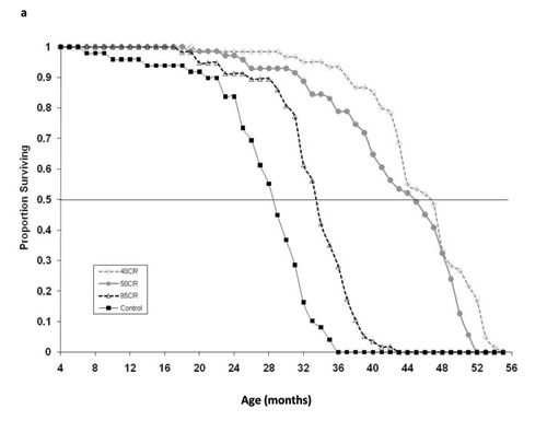
Figure 1: Survival curves for four treatment groups in the caloric restriction experiment of Weindruch et al. (1986): Control (ad libitum) and 85, 50 and 40 kcal/week feeding treatments.
Symbols are the observed mortality rates, lines are the Gompertz maximum likelihood models.
© 2010 Nature Education All rights reserved. 
We obtained the raw data from the authors in the form of "age-at-death," fit mortality models and performed hypothesis testing in program WinModest (Pletcher 1999). We fit the Gompertz model to the age-at-death data and estimated the two parameters for the Gompertz model (IMR and RoA) for each of the four treatment groups. Control mice had the highest IMR, the measure of "frailty." However, the ordering of IMR for the other groups did not match the ordering of median and maximum life span (Table 1; Figure 2). The group with the lowest IMR was in fact the 85 kcal/week treatment group. The 50 and 40 kcal groups were in between the control and the 85 kcal animals. Examining estimates of the Gompertz rate-of-aging parameter (RoA), we found that the 85 kcal group and the control group aged faster than the 40 and 50 kcal treatment groups. We further estimated a useful index of aging, the mortality rate doubling times (MRDT), which is a simple transformation RoA that includes units of time (MRDT = ln(2)/RoA) (see Finch et al. 1990). The 85 kcal and control groups had MRDTs of 2.78 months and 2.9 months, respectively. And the MRDTs of the 40 and 50 kcal groups were 3.4 and 3. 95 months, respectively. The practical conclusions from these analyses are that:
- the effects of caloric restriction on IMR (frailty) were not predicted by the amount of dietary restriction and did not follow the ranking suggested by the survival curves (Figure 1);
- similarly, the effects of caloric restriction on RoA did not rank order with amount of dietary restriction.
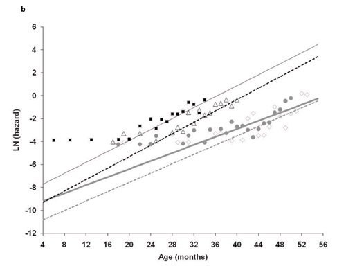
Figure 2: Ln (instantaneous mortality rate) for the same four treatment groups
Symbols are the observed mortality rates, lines are the Gompertz maximum likelihood models.
© 2010 Nature Education All rights reserved.
In other words, the control and 85 kcal groups had equivalent rates of aging, and aging was slowest in the 50 kcal treatment group (not the 45 kcal group as suggested by the survival curves).
|
Treatment
|
Median
|
IMR (mo-1)
|
RoA
|
MRDT (mo)
|
Change-in-Median (%)
|
|
Control |
34 |
0.00044 |
0.239 |
2.90 |
- |
| 85.0 |
34 |
0.00009 |
0.250 |
2.78 |
17.2 |
| 50.0 |
45 |
0.0001 |
0.176 |
3.95 |
55.2 |
|
40.0 |
47 |
0.00002 |
0.203 |
3.41 |
62.1 |
| Table 1: Estimates of mortality parameters for a mouse caloric restriction study by Weindruch et al. (1986) Notes: Median (in months) is the age at which survival lx = 0.5; initial mortality (per month) is the IMR parameter from the Gompertz equation (μx = IMR*e(RoA*x)); slope (RoA) represents the rate of aging parameter from the Gompertz model; MRDT is the mortality rate doubling time (in months), where MRDT = ln(2)/RoA. | |||||
Summary
This case study highlights the general issues raised earlier. First, that maximum lifespan is not an easily obtainable metric. Specifically, it is unambiguous in the sense that once the last animal dies, it is most definitely dead. But to estimate the variance in maximum lifespan, many replicate populations would need to be followed for each treatment group (with each replicate providing a single observation of maximum lifespan). Second, median lifespan, although measurable from a single population, provides no information on the age-specificity and patterns in age-specific vital rates that are contributing to differences in "aging" (i.e., differences in physiological frailty and rates of increasing mortality across the adult lifespan). Finally, our partitioning of aging into two components — IMR and RoA — allows us to unravel causation in a demographic sense. Specifically, it allows us to specify an aging rate that is separate from its starting value (IMR), independent of fluctuations in survival due to temporary experimental impacts, and not necessarily equivalent to expectations due to median or maximum lifespan.
References and Recommended Reading
Arias, E. United States Life Tables, 2004. Hyattsville, MA: National Center for Health Statistics, 2007.
Bronikowski, A. M. et al. The aging baboon: Comparative demography in a non-human primate. Proceedings of the National Academy of Sciences of the United States of America 99, 9591–9595 (2002).
Bronikowski, A. M. et al. The evolution of aging and age-related physical decline in mice selectively bred for high voluntary exercise. Evolution 60, 1494–1508 (2006).
Carey, J. R. Longevity: The Biology and Demography of Life Span. Princeton, NJ: Princeton University Press, 2003.
Chiang, C. L. The Life Table and its Applications. Malabar, FL: Krieger, 1984.
Finch, C. Longevity, Senescence and the Genome. Chicago, IL: University of Chicago Press, 1990.
Finch, C. E., Pike, M. C., & Witten, M. Slow mortality rate accelerations during aging in some animals approximate that of humans. Science 249, 902–905 (1990).
Gems, D., Pletcher, S., & Partridge, L. Interpreting interactions between treatments that slow aging. Aging Cell 1, 1–9 (2002).
Gompertz, B. On the nature of the function expressive of the law of human mortality, and on a new mode of determining the value of life contingencies. Philosophical Transactions of the Royal Society London 115, 513–583 (1825).
Kenyon, C. The genetics of ageing. Nature 464, 504–512 (2010).
Lutz, W., Sanderson, W., & Scherbov, S. The coming accleration of global population ageing. Nature 451, 716–719 (2008).
Machin, D., Cheung, Y. B., & Parmer, M. K. N. Survival Analysis: A Practical Approach. Chichester, UK: John Wiley & Sons, 2006.
Pletcher, S. D. Model fitting and hypothesis testing for age-specific mortality data. Journal of Evolutionary Biology 12, 430–439 (1999).
Pletcher, S. D., Khazaeli, A. A., & Curtsinger, J. W. Why do life spans differ? Partitioning mean longevity differences in tems of age-specific mortality parameters. Journal of Gerontology A: Biological Sciences 55, B381–B389 (2000).
Promislow, D. E. L. & Bronikowski, A. M. "The evolutionary genetics of senescence." In Evolutionary Genetics: Concepts and Case Studies, eds. J. Wolf & C. Fox (Oxford, UK: Oxford University Press, 2006): 464–481.
Rose, M. R. Evolutionary Biology of Aging, Oxford, UK & New York, NY: Oxford University Press, 1991.
Sacher, G. A. "Life table modification and life prolongation." In Handbook of the Biology of Aging, eds. C. E. Finch & L. Hayflick (New York, NY: Van Nostrand Reinhold Company, 1977): 582-638.
Vaupel, J. W. Biodemography of human ageing. Nature 464, 536–541 (2010).
Weindruch, R. et al. The retardation of aging in mice by dietary restriction: longevity, cancer, immunity, and lifetime energy-intake. Journal of Nutrition 116, 641–654 (1986).
Wilmoth, J. R. "In search of limits." In Between Zeus and the Salmon: The Biodemography of Longevity, eds. K. W. Wachter & C. E. Finch (Washington, DC: National Academy Press, 1997): 38–64.