
Abstract
We report significant relations between past changes in the market correlation structure and future changes in the market volatility. This relation is made evident by using a measure of “correlation structure persistence” on correlation-based information filtering networks that quantifies the rate of change of the market dependence structure. We also measured changes in the correlation structure by means of a “metacorrelation” that measures a lagged correlation between correlation matrices computed over different time windows. Both methods show a deep interplay between past changes in correlation structure and future changes in volatility and we demonstrate they can anticipate market risk variations and this can be used to better forecast portfolio risk. Notably, these methods overcome the curse of dimensionality that limits the applicability of traditional econometric tools to portfolios made of a large number of assets. We report on forecasting performances and statistical significance of both methods for two different equity datasets. We also identify an optimal region of parameters in terms of True Positive and False Positive trade-off, through a ROC curve analysis. We find that this forecasting method is robust and it outperforms logistic regression predictors based on past volatility only. Moreover the temporal analysis indicates that methods based on correlation structural persistence are able to adapt to abrupt changes in the market, such as financial crises, more rapidly than methods based on past volatility.
Introduction
Forecasting changes in volatility is essential for risk management, asset pricing and scenario analysis. Indeed, models for describing and forecasting the evolution of volatility and covariance among financial assets are widely applied in industry1,2,3,4. Among the most popular approaches are worth mentioning the multivariate extensions of GARCH5, the stochastic covariance models6 and realized covariance7. However most of these econometrics tools are not able to cope with more than few assets, due to the curse of dimensionality and the increase in the number of parameters1, limiting their insight into the volatility evolution to baskets of few assets only. This is unfortunate, since gathering insights into systemic risk and the unfolding of financial crises require modelling the evolution of entire markets which are composed by large numbers of assets1.
We suggest to use network filtering8,9,10,11,12,13,14 and metacorrelation as valuable tools to overcome this limitation. Correlation-based filtering networks are tools which have been widely applied to filter and reduce the complexity of covariance matrices made of large numbers of assets (of the order of hundreds), representative of entire markets. This strand of research represents an important part of the Econophysics literature and has given important insights for risk management, portfolio optimization and systemic risk regulation15,16,17,18,19,20.
The volatility of a portfolio depends on the covariance matrix of the corresponding assets21. Therefore, the latter can provide insights into the former. In this work we elaborate on this connection showing that correlation matrices can be used to predict variations of volatility. The approach we propose exploits network filtering to explicitly predict future volatility of markets made of hundreds of stocks. This is quite an innovative use of correlation-based networks, which have been so far mostly used for descriptive analyses, with the connections with risk forecasting being mostly overlooked. Some works have shown that is possible to use dimensionality reduction techniques, such as spectral methods22, as early-warning signals for systemic risk23,24: however these approaches, although promising, do not provide proper forecasting tools, as they are affected by high false positive ratios and are not designed to predict a specific quantity.
We quantify the rate of change in the structure of the market correlation matrix by using two tools: (1) the “correlation structure persistence” 〈ES〉 which is a measure of similarity between past correlation structures computed from network filtering; (2) the metacorrelation, that is the correlation between correlation matrices at different times; we discuss performances, advantages and disadvantages of the two approaches. We show how such measures exhibit significant predicting power on the market volatility, providing a tool to forecast it. We assess the reliability of these forecasting through out-of-sample tests on two different equity datasets.
The rest of this paper is structured as follows: we first describe the two datasets we have analysed and we introduce the correlation structure persistence and metacorrelation; then we show how our analyses point out a strong interdependence between correlation structure persistence and future changes in the market volatility; moreover, we describe how this result can be exploited to provide a forecasting tool useful for risk management, by presenting out-of-sample tests and false positive analysis; then we investigate how the forecasting performance changes in time; finally we discuss our findings and their theoretical implications.
Results
We have analysed two different datasets of equity data. The first set (NYSE dataset) is composed by daily closing prices of N = 342 US stocks traded in New York Stock Exchange, covering 15 years from 02/01/1997 to 31/12/2012. The second set (LSE dataset) is composed by daily closing prices of N = 214 UK stocks traded in the London Stock Exchange, covering 13 years from 05/01/2000 to 21/08/2013. All stocks have been continuously traded throughout these periods of time. These two sets of stocks have been chosen in order to provide a significant sample of the different industrial sectors in the respective markets.
For each asset i (i = 1, ..., N) we have calculated the corresponding daily log-return ri(t) = log (Pi(t)) − log (Pi(t − 1)), where Pi(t) is the asset i price at day t. The market return rM(t) is defined as the average of all stocks returns: rM(t) = 1/N∑iri(t). In order to calculate the correlation between different assets we have then analysed the observations by using n moving time windows, Ta with a = 1, ..., n. Each time window contains θ observations of log-returns for each asset, totaling to N × n observations. The shift between adjacent time windows is fixed to dT = 5 trading days: therefore, adjacent time windows share a significant number of observations. We have calculated the correlation matrix within each time window, {ρij(Ta)}, by using an exponential smoothing method25 that allows to assign more weight on recent observations. The smoothing factor of this scheme has been chosen equal to θ/3 according to previously established criteria25.
A measure of correlation structure persistence with filtering networks
From each correlation matrix {ρij(Ta)} we computed the corresponding Planar Maximally Filtered Graph (PMFG)26 which is one realization of a broader class of filtering networks associating a sparse graph to a correlation matrix27. Specifically, the PMFG is a sparse network representation of the correlation matrix that retains only a subset of most significant entries, selected through the topological criterion of being maximally planar9. In general, any correlation matrix can be represented as a graph, where each node is an asset and each link between two nodes represents the correlation between them. From this network, which is typically fully connected, several different planar graphs can be extracted as subgraphs: a graph is planar if it can be embedded on a plane without link crossing26. The Planar Maximally Filtered Graph (PMFG) is the planar graph associated with the original correlation matrix which maximizes the sum of weights accordingly with a given greedy algorithm26. The PMFG can be seen as a generalization of the Minimum Spanning Tree: the PMFG is able to retain a higher amount of information9, having a less strict topology constraint allowing to keep a larger number of links. Moreover, the MST is a subgraph of PMFG. In terms of computational complexity the algorithm that builds PMFG is O(N3); recently27 a new algorithm has been proposed, able to build a chordal planar graph (called Triangulated Maximally Filtered Graph, TMFG) with an execution time O(N2), making possible a much higher scalability and the application to Big Data27. Such networks have been shown to provide a deep insight into the dependence structure of financial assets9,10,28.
Once the n PMFGs, G(Ta) with a = 1, ..., n, have been computed we have calculated a measure that monitors the correlation structure persistence, based on a measure of PMFG similarity. This measure, that we call ES(Ta, Tb), computes the edges in common between a PMFG computed over the time-windows Ta and Tb of length θ. Its average over a set of L windows Tb (see Fig. 1 and Eqs 2 and 3 in Methods) is denoted with 〈ES〉(Ta). This measure uses past data only and indicates how slowly the correlation structure measured at time window Ta is differentiating from structures associated to previous time windows.

Scheme of time windows setting for 〈ES〉(Ta) and q(Ta) calculation.
Ta is a window of length θ. The correlation structure persistence 〈ES〉(Ta) (upper axis) is computed by using data in Ta and in the first L time windows before Ta. The volatility ratio q(Ta) is computed by using data in Ta and in the future time window  . In the upper axis the time windows are actually overlapping, but they are here represented as disjoint for the sake of simplicity.
In Fig. 2 we show the ES(Ta, Tb) matrices (Eq. 3) for the NYSE and LSE dataset, for θ = 1000. We can observe a block structure with periods of high structural persistence and other periods whose correlation structure is changing faster. In particular two main blocks of high persistence can be found before and after the 2007–2008 financial crisis; a similar result was found in a previous work20 with a different measure of similarity. These results are confirmed for all values of θ considered.

ES(Ta, Tb) matrices for θ = 1000, for NYSE (left) and LSE dataset (right).
A block-like structure can be observed in both datasets, with periods of high structural persistence and other periods whose correlation structure is changing faster. The 2007–2008 financial crisis marks a transition between two main blocks of high structural persistence.
A measure of correlation structure persistence with metacorrelations
We have considered a more direct measure of correlation structure persistence, the metacorrelation z(Ta, Tb), that is the Pearson correlation computed between the coefficients of correlation matrices at Ta and Tb (see Methods for more details). Such measure does not make use of any filtering network. Let us note that, although conceptually simpler, this measure requires an equivalent computational complexity (O(N 2)) than 〈ES〉(Ta) (when computed with the TMFG approach27) but it requires a larger memory usage. Figure 3 displays the similarity matrices obtained with this measure for NYSE and LSE datasets: we can observe again block-like structures, that however carry different information from the ES(Ta, Tb) in Fig. 2; in particular, blocks show higher intra-similarity and less structure. Similarly to the construction of ES(Ta). we have defined 〈z〉(Ta) as the weighted average over L past time windows (see Methods Eqs 2 and 5).

z(Ta, Tb) matrices for θ = 1000, for NYSE (left) and LSE dataset (right).
A block-like structure can be observed in both datasets, with periods of high structural persistence and other periods whose correlation structure is changing faster. The blocks of high similarity show higher compactness than in Fig. 2.
A forward looking measure of volatility: volatility ratio
The volatility ratio q(Ta)29,30 is a foward-looking measure that, at each time window Ta, compute the ratio between the estimated volatility in the following time-window  and the one estimated from Ta. Unlike 〈ES〉(Ta) or 〈z〉(Ta) the value of q(Ta) is not known at the end of Ta as it requires information from the next time-window. Figure 1 shows a graphical representation of the time window set-up.
Interplay between correlation structure persistence and volatility ratio
To investigate the relation between 〈ES〉(Ta) and q(Ta) we have calculated the two quantities with different values of θ and L in Eqs 2 and 6, to assess the robustness against these parameters. Specifically, we have used θ ∈ (250, 500, 750, 1000) trading days, that correspond to time windows of length 1, 2, 3 and 4 years respectively; L ∈ (10, 25, 50, 100), that correspond (given dT = 5 trading days) to an average in Eq. 2 reaching back to 50, 125, 250 and 500 trading days respectively. θforward has been chosen equal to 250 trading days (one year) for all the analysis.
In Fig. 4 we show 〈ES〉(Ta) and q(Ta) as a function of time, for θ = 1000 and L = 100. As expected, main peaks of q(Ta) occur during the months before the most turbulent periods in the stock market, namely the 2002 market downturn and the 2007–2008 credit crisis. Interestingly, the corresponding 〈ES〉(Ta) seems to follow a specular trend. This is confirmed by explicit calculation of Pearson correlation between the two signals, reported in Tables 1 and 2: as one can see, for all combinations of parameters the correlation is negative.

〈ES〉(Ta) and q(Ta) signals represented for θ = 1000 and L = 100, for both NYSE (left graph) and LSE (right graph) datasets.
It is evident the anticorrelation between the two signals. The financial crisis triggers a major drop in the structural persistence and a corresponding peak in q(Ta).
In order to check the significance of this anticorrelation we cannot rely on standard tests on Pearson coefficient, such as Fisher transform31, as they assume i.i.d. series32. Both 〈ES〉(Ta) and q(Ta) are instead strongly autocorrelated, due to the significant overlapping between adjacent time windows. In Supplementary Material, Fig. S3, the autocorrelation of q(Ta) is analysed at different lags. Therefore we have calculated confidence intervals by performing a block bootstrapping test33. This is a variation of the bootstrapping test34, conceived to take into account the autocorrelation structure of the bootstrapped series. The only free parameter in this method is the block length, that we have chosen applying the optimal selection criterion proposed in literature35: such criterion is adaptive on the autocorrelation strength of the series as measured by the correlogram. We have found, depending on the parameters θ and L, optimal block lengths ranging from 29 to 37, with a mean of 34 (corresponding to 170 trading days). By performing block bootstrapping tests we have therefore estimated confidence intervals for the true correlation between 〈ES〉(Ta) and q(Ta); in Tables 1 and 2 correlations whose 95% and 99% confidence intervals (CI) do not include zero are marked with one and two stars respectively. As we can see, 14 out of 16 correlation coefficients are significantly different from zero within 95% CI in the NYSE dataset, and 12 out of 16 in the LSE dataset. For what concerns the 99% CI, we observe 13 out of 16 for the NYSE and 9 out of 16 for the LSE dataset. Non-significant correlations appear only for θ = 250, suggesting that this length is too small to provide a reliable measure of structural persistence. Very similar results are obtained by using Minimum Spanning Tree (MST)36 instead of PMFG as network filtering.
Given the interpretation of 〈ES〉(Ta) and q(Ta) given above, anticorrelation implies that an increase in the “speed” of correlation structure evolution (low 〈ES〉(Ta)) is likely to correspond to underestimation of future market volatility from historical data (high q(Ta)), whereas when the structure evolution “slows down” (high 〈ES〉(Ta)) there is indication that historical data is likely to provide an overestimation of future volatility. This means that we can use 〈ES〉(Ta) as a valuable predictor of current historical data reliability. This result is to some extent surprising as 〈ES〉(Ta) is derived from PMFGs topology, which in turns depends only on the ranking of correlations and not on their actual value: yet, this information provides meaningful information about the future market volatility and therefore about the future covariance.
In Tables 3 and 4 we show the correlation between 〈z〉(Ta) and q(Ta). As we can see, although an anticorrelation is present for each combination of parameters θ and L, correlation coefficients are systematically closer to zero than in Tables 1 and 2, where 〈ES〉(Ta) was used. Moreover the number of significant Pearson coefficients, according to the block bootstrapping, decreases to 12 out of 16 in NYSE and to 10 out of 16 in LSE dataset. Since 〈z〉(Ta) does not make use of PMFG, this result suggests that the filtering procedure associated to correlation-based networks is enhancing the relation between past correlation structure and future volatility changes. We shall however see in the next session that for forecasting purposes network filtering might not be always beneficial.
Forecasting volatility with correlation structure persistence
In this section we evaluate how well the correlation structure persistence 〈ES〉(Ta) can forecast the future through its relation with the forward-looking volatility ratio q(Ta). In particular we focus on estimating whether q(Ta) is greater or less than 1: this information, although less complete than a precise estimation of q(Ta), gives us an important insight into possible overestimation (q(Ta) < 1) or underestimation (q(Ta) > 1) of future volatility. The equivalent assessment of forecasting power of 〈z〉(Ta) is reported in Supplementary Material (Tables S1–S4 and Fig. S1).
We have proceeded as follows. Given a choice of parameters θ and L, we have calculated the corresponding set of pairs {〈ES〉(Ta), q(Ta)}, with a = 1, ..., n. Then we have defined Y(Ta) as the categorical variable that is 0 if q(Ta) < 1 and 1 if q(Ta) > 1. Finally we have performed a logistic regression of Y(Ta) against 〈ES〉(Ta): namely, we assume that37:

where S(t) is the sigmoid function  38; we estimate parameters β0 and β1 from the observations {〈ES〉(Ta), q(Ta)}a=1, ... ,n through Maximum Likelihood39.
Once the model has been calibrated, given a new observation 〈ES〉(Tn+1) = x we have predicted Y(Tn+1) = 1 if P{Y(Tn+1) = 1|〈ES〉(Tn+1) = x} > 0.5, and Y(Tn+1) = 0 otherwise. This classification criterion, in a case with only one predictor, corresponds to classify Y(Tn+1) according to whether 〈ES〉(Tn+1) is greater or less than a threshold r which depends on β0 and β1, as shown in Fig. 5 (right graphs) for a particular choice of parameters. Therefore the problem of predicting whether market volatility will increase or decrease boils down to a classification problem39 with 〈ES〉(Ta) as predictor and Y(Ta) as target variable.

Partition of data into training (left graphs) and test (right graphs) set.
Training sets are used to regress Y(Ta) against 〈ES〉(Ta), in order to estimate the coefficents in the logistic regression and therefore identify the regression threshold, shown as a vertical continuous line. The test sets are used to test the forecasting performance of such regression on a subset of data that has not been used for regression; the model predicts Y(Ta) = 1 (q(Ta) > 1, blue squares in the figure) if 〈ES〉(Ta) is less than the regression threshold, and Y(Ta) = 0 (q(Ta) < 1, red stars in the figure) otherwise.
We have made use of a logistic regression because it is more suitable than a polynomial model for dealing with classification problems37. Other classification algorithms are available; we have chosen the logistic regression due to its simplicity. We have also implemented the KNN algorithm39 and we have found that it provides similar outcomes but worse results in terms of the forecasting performance metrics that we discuss in this section.
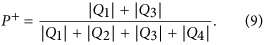
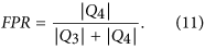
We have then evaluated the goodness of the logistic regression at estimating Y(Tn+1) given a new observation 〈ES〉(Tn+1). To this end, we have computed three standard metrics for assessing the performance of a classification method: the probability of successful forecasting P+, the True Positive Rate TPR and the False Positive Rate FPR. P+ represents the expected fraction of correct predictions, TPR is the method goodness at identifying true positives (in this case, actual increases in volatility) and FPR quantifies the method tendency to false positives (predictions of volatility increase when the volatility will actually decrease): see Methods for more details. Overall these metrics provide a complete summary of the model goodness at predicting changes in the market volatility37.
In order to avoid overfitting we have estimated the metrics above by means of an out-of-sample procedure37,39. We have divided our dataset into two periods, a training set and a test set. In the training set we have calibrated the logistic equation in Eq. 1, estimating the parameters β0 and β1; in the test set we have used the calibrated model to measure the goodness of the model predictions by computing the measures of performance in Eqs 9, 10, 11. In Fig. 5 this division is shown for a particular choice of θ and L, for both NYSE and LSE dataset. In this example the percentage of data included in the test set (let us call it ftest) is 30%.
Probabilities of successful forecasting P+ are reported in Tables 5 and 6, for ftest = 30%. As we can see P+ is higher than 50% for all combinations of parameters in NYSE dataset, and in almost all combinations for LSE dataset. Stars mark those values of P+ that are significantly higher than the same probability obtained by using the most recent value of q instead of 〈ES〉(Ta) as a predictor for q(Ta) in the logistic regression (let us call  such probability, reported in Tables S5 and 6 in Supplementary Material). Specifically, we have defined a null model where variations from such probability
  are due to random fluctuations only; given n observations, such fluctuations follow a Binomial distribution
  , with mean
  and variance
  . Then p-values have been calculated by using this null distribution for each combination of parameters. This null hypothesis accounts for the predictability of q(Ta) that is due to the autocorrelation of q(Ta) only; therefore P+ significantly higher than the value expected under this hypothesis implies a forecasting power of 〈ES〉(Ta) that is not explained by the autocorrelation of q(Ta). From the table we can see that P+ is significant in 12 out of 16 combinations of parameters for NYSE dataset, and in 13 out of 16 for LSE dataset. This means that correlation persistence is a valuable predictor for future average correlation, able to outperform forecasting method based on past average correlation trends. These results are robust against changes of ftest, as long as the training set is large enough to allow an accurate calibration of the logistic regression. We have found this condition is satisfied for ftest < 40%. In Supplementary Material, Fig. S3 reports the autocorrelation of q(Ta). We also investigated a null model that uses the weighted average version of q(Ta): results are very similar and reported in Supplementary Material (Tables S9 and 10).
It must be noted that P+ does not give any information on the method ability to distinguish between true and false positives. To investigate this aspect we need TPR and FPR. A traditional way of representing both measures from a binary classifier is the so-called “Receiver operating characteristic” (ROC) curve40. In a ROC plot, TPR is plotted against FPR as the discriminant threshold is varied. The discriminant threshold pmax is the value of the probability in Eq. 1 over which we classify Y(Ta) = 1: the higher pmax is, the less likely the method is to classify Y(Ta) = 1 (in the analysis on P+ we chose pmax = 0.5). Ideally, a perfect classifier would yield TPR = 1 for all pmax > 0, whereas a random classifier is expected to lie on the line TPR = FPR. Therefore a ROC curve which lies above the line TPR = FPR indicates a classifier that is better than chance at distinguishing true from false positives37.
As one can see from Fig. 6, the ROC curve's position depends on the choice of parameters θ and L. In this respect our classifier performs better for low values of L and θ. This can be quantified by measuring the area under the ROC curve; such measure, often denoted by AUC37, is shown in Tables 7 and 8. For both datasets the optimal choice of parameters is θ = 500 and L = 10. In Supplementary Material, Tables S7 and 8 and Fig. S4, the ROC curve and AUC values are reported for the case when q(Ta) is used as predictor, showing that q(Ta) underperforms 〈ES〉(Ta) in terms of ROC analysis as well.

Receiver operating characteristic (ROC) curve.
Left graph: True positive rate (TPR) against False positive rate (FPR) as the discriminant threshold pmax of the classifier is varied, for each combination of parameters θ and L in the NYSE dataset. The closer the curve is to the upper left corner of each graph, the better is the classifier compared to chance. Right graph: True positive rate (TPR) against False positive rate (FPR) as the discriminant threshold pmax of the classifier is varied, for each combination of parameters θ and L in the LSE dataset.
We also tested the predictive power of metacorrelations z(Ta, Tb) (see Supplementary Material). By comparing with the results for ES(Ta, Tb) we observed that 〈z〉(Ta) has almost always a slightly higher P+ than 〈ES〉(Ta) in the NYSE dataset, whereas on average it has lower values than 〈ES〉(Ta) in the LSE dataset (with 9 out of 16 values of P+ less than the corresponding 〈ES〉(Ta) probabilities). On the other hand, the ROC analysis shows that the predictor 〈ES〉(Ta) performs better than 〈z〉(Ta) in the NYSE dataset and worse in the LSE dataset. Results for forecasting with z(Ta, Tb) are reported in Section S.1 of Supplementary Material (Tables S1 and S4 and Fig. S1). We therefore conclude that the advantage of network filtering in measuring the correlation structure persistence is clear only when it comes to the correlation analysis with q(Ta), whereas for the forecasting model it might be convenient to use one measure or the other depending on whether one wants to maxmise the probability of forecasting (P+) or minimise the impact of false positive (ROC analysis).
Temporal evolution of forecasting performance
In this section we look at how the forecasting performance changes at different time periods. In order to explore this aspect we have counted at each time window Ta the number N+(Ta) of Y(Ta) predictions (out of the 16 predictions corresponding to as many combinations of θ and L) that have turned out to be correct; we have then calculated the fraction of successful predictions n+(Ta) as n+(Ta) = N+(Ta)/16. In this way n+(Ta) is a proxy for the goodness of our method at each time window. Logistic regression parameters β0 and β1 have been calibrated by using the entire time period as training set, therefore this is an in-sample analysis.
In Fig. 7 we show the fraction of successful predictions for both NYSE and LSE datasets (upper graphs, blue circles). For comparison we also show the same measure obtained by using the most recent value of q(Ta) as predictor (bottom graphs); as in the previous section, it represents a null model that makes prediction by using only the past evolution of q(Ta). As we can see, both predictions based on 〈ES〉(Ta) and on past values of q(Ta) display performances changing in time. In particular n+(Ta) drops just ahead of the main financial crises (the market downturn in March 2002, 2007–2008 financial crisis, Euro zone crisis in 2011); this is probably due to the abrupt increase in volatility that occurred during these events and that the models took time to detect. After these drops though performances based on 〈ES〉(Ta) recover much more rapidly than those based on past value of q(Ta). For instance in the first months of 2007 our method shows quite high n+(Ta) (more than 60% of successful predictions), being able to predict the sharp increase in volatility to come in 2008 while predictions based on q(Ta) fail systematically until 2009. Overall, predictions based on correlation structure persistence appear to be more reliable (as shown by the average n+(Ta) over all time windows, the horizontal lines in the plot) and faster at detecting changes in market volatility. Similar performances to 〈ES〉(Ta) can be observed when n+(Ta) is calculated using 〈z〉(Ta) as measure of correlation structure persistence (see Supplementary Material, Fig. S2).

Fraction of successful predictions as a function of time.
NYSE (left graph) and LSE dataset (right graph). Forecasting is based on logistic regression with predictor 〈ES(Ta)〉 (top graphs) and most recent value of q(Ta) (bottom graphs). Horizontal lines represent the average over the entire period.
Discussion
In this paper we have proposed a new tool for forecasting market volatility based on correlation-based information filtering networks, metacorrelation and logistic regression, useful for risk and portfolio management. The advantage of our approach over traditional econometrics tools, such as multivariate GARCH and stochastic covariance models, is the “top-down” methodology that treats correlation matrices as the fundamental objects, allowing to deal with many assets simultaneously; in this way the curse of dimensionality, that prevents e.g. multivariate GARCH to deal with more than few assets, is overcome. We have proven the forecasting power of this tool by means of out-of-sample analyses on two different stock markets; the forecasting performance has been proven to be statistically significant against a null model, outperforming predictions based on past market correlation trends. Moreover we have measured the ROC curve and identified an optimal region of the parameters in terms of True Positive and False Positive trade-off. The temporal analysis indicates that our approach, based on correlation structure persitance, is able to adapt to abrupt changes in the market, such as financial crises, more rapidly than methods based on past volatility.
This forecasting tool relies on an empirical fact that we have reported in this paper for the first time. Specifically, we have shown that there is a deep interplay between future changes in market volatility and the rate of change of the past correlation structure. The statistical significance of this relation has been assessed by means of a block-bootstrapping technique. An analysis based on metacorrelation has revealed that this interplay is better highlighted when filtering based on correlation filtering graphs (Planar Maximally Filtered Graphs) is used to estimate the correlation structure persistence. However, when it comes to forecasting performances, metacorrelation might be preferable to network filtering On the other hand, the use of planar graphs allows a better visualisation of the system, making possible a clearer interpretation of correlation structure changes. We must note that correlation filtering networks retain a much smaller amount of information than the whole correlation matrix and nonetheless reveal larger relations with future volatility changes and comparable forecasting performances. This could be crucial for a possible use of this tools in the context of big-data analytic where several thousands of indicators are simultaneously considered.
This finding sheds new light into the dynamic of correlation. Both metacorrelation and the topology of correlation filtering networks depend on the ranking of the N(N − 1)/2 pairs of cross-correlations; therefore a decrease in the correlation structure persistence points out a faster change of this ranking. Our result indicates that such increase is typically followed by a rise in the market volatility, whereas decreases are followed by drops. A possible interpretation of this is related to the dynamics of risk factors in the market. Indeed higher volatility in the market is associated to the emergence of a (possibly new) risk factor that makes the whole system unstable; such transition could be anticipated by a quicker change of the correlation ranking, triggered by the still emerging factor and revealed by the correlation structure persistence. Such persistence can therefore be a powerful tool for monitoring the emergence of new risks, valuable for a wide range of applications, from portfolio management to systemic risk regulation. Moreover this interpretation would open interesting connections with those approaches to systemic risk that make use of Principal Component Analysis, monitoring the emergence of new risk factors by means of spectral methods23,24. We plan to investigate all these aspects in a future work.
Methods
Correlation structure persistence with filtering networks 〈ES〉(Ta)
We define the correlation structure persistence at time Ta as:

where  is an exponential smoothing factor, L is a parameter and ES(Ta, Tb) is the fraction of edges in common between the two PMFGs G(Ta) and G(Tb), called “edge survival ratio”15. In formula, ES(Ta,Tb) reads:

where Nedges is the number of edges (links) in the two PMFGs (constant and equal to 3N − 6 for a PMFG26), and  (
( ) represents the edge-sets of PMFG at Ta (Tb). The correlation structure persistence 〈ES〉(Ta) is therefore a weighted average of the similarity (as measured by the edge survival ratio) between G(Ta) and the first L previous PMFGs, with an exponential smoothing scheme that gives more weight to those PMFGs that are closer to Ta. The parameter ω0 in Eq. 2 can be calculated by imposing
  . Intuitively, 〈ES〉(Ta) measures how slowly the change of correlation structure is occurring in the near past of Ta.
Correlation structure persistence with metacorrelation 〈z〉(Ta)
Given two correlation matrices {ρij(Ta)} and {ρij(Tb)} at two different time windows Ta and Tb, their metacorrelation z(Ta,Tb) is defined as follows:

where 〈...〉ij is the average over all couples of stocks i, j. Similarly to Eq. 2 we have then defined z(Ta) as the weighted average over L past time windows:

Volatility ratio q(Ta)
In order to quantify the agreement between the estimated and the realized risk we here make use of the volatility ratio, a measure which has been previously used29,41 for this purpose and defined as follows:

where  is the realized volatility of the average market return rM(t) computed on the time window
  ; σ(Ta) is the estimated volatility of rM(t) computed on time window Ta, by using the same exponential smoothing scheme25 described for the correlation {ρij(Ta)}. Specifically,
  is the time window of length θforward that follows immediately Ta: if tθ is the last observation in Ta,
  covers observations from tθ+1 to
  (Fig. 1). Therefore the ratio in Eq. 6 estimates the agreement between the market volatility estimated with observations in Ta and the actual market volatility observed over an investment in the N assets over
  . If q(Ta) > 1, then the historical data gathered at Ta has underestimated the (future) realized volatilty, whereas q(Ta) < 1 indicates overestimation. Let us stress that q(Ta) provides an information on the reliability of the covariance estimation too, given the relation between market return volatility and covariance21:


where Covij(Ta) and  are respectively the estimated and realized covariances.
Measures of classification performance
With reference to Fig. 5b,d, let us define the number of observations in each quadrant Qi (i = 1, 2, 3, 4) as |Qi|. In the terminology of classification techniques39, |Q1| is the number of True Positive (observations for which the model correctly predicted Y(Ta) = 1), |Q3| is the number of True Negative (observations for which the model correctly predicted Y(Ta) = 0), |Q2| the number of False Negative (observations for which the model incorrectly predicted Y(Ta) = 0) and |Q4| the number of False Positive (observations for which the model incorrectly predicted Y(Ta) = 1). We have then computed the following measures of quality of classification, that are the standard metrics for assessing the performances of a classification method39:
-
Probability of successful forecasting (P+)39: represents the method probability of a correct prediction, expressed as fraction of observed 〈ES〉(Ta) values through which the method has successfully identified the correspondent value of Y(Ta). In classification problems, sometimes, the error rate I is used37, which is simply I = 1 − P+. P+ is computed as follows:
-
True Positive Rate (TPR)39: it is the probability of predicting Y(Ta) = 1, conditional to the fact that the real Y(Ta) is indeed 1 (that is, to predict an increase in volatility when the volatility will indeed increase); it represents the method sensitivity to increase in volatility. It is also called “recall”37. In formula:

-
False Positive Rate (FPR)39: it is the probability of predicting Y(Ta) = 1, conditional to the fact that the real Y(Ta) is instead 0 (that is, to predict an increase in volatility when the volatility will actually decrease). It is also called “1-specificity”37. In formula:


Additional Information
How to cite this article: Musmeci, N. et al. Interplay between past market correlation structure changes and future volatility outbursts. Sci. Rep. 6, 36320; doi: 10.1038/srep36320 (2016).
Publisher’s note: Springer Nature remains neutral with regard to jurisdictional claims in published maps and institutional affiliations.
References
Daníelsson, J. Financial risk forecasting (Wiley, 2011).
Hafner, C. M. & Manner, H. Multivariate time series models for asset prices. Handbook of Computational Finance 89–115 (2012).
Bouchaud, J.-P. & Potters, M. Theory of Financial Risk and Derivative Pricing: From Statistical Physics to Risk Management (Cambridge, 2000).
Preis, T., Kenett, D. Y., Stanley, H. E., Helbing, D. & Ben-Jacob, E. Quantifying the behavior of stock correlations under market stress. Scientific Reports 2, 752 (2012).
Bauwens, L., Laurent, S. & Rombouts, J. Multivariate GARCH models: a survey. Journal of Applied Econometrics 21, 79–109 (2006).
Clark, P. A subordinate stochastic process model with finite variance for speculative prices. Econometrica 41, 135–155 (1973).
Andersen, T., Bollerslev, T., Diebold, F. & Labys, P. Forecasting realized volatility. Econometrica 71(2), 579–625 (2003).
Mantegna, R. N. Hierarchical structure in financial markets. Eur. Phys. J. B 11, 193 (1999).
Tumminello, M., Aste, T., Di Matteo, T. & Mantegna, R. A tool for filtering information in complex systems. Proc. Natl. Acad. Sci. 102, 10421–10426 (2005).
Aste, T. & Matteo, T. D. Dynamical networks from correlations. Physica A 370, 156–161 (2006).
Onnela, J. P., Chakraborti, A., Kaski, K., Kertész, J. & Kanto, A. Asset trees and asset graphs in financial markets. Phys. Scr. T106, 48 (2003).
Onnella, J.-P., Kaski, K. & Kertész, J. Clustering and information in correlation based financial networks. Eur. Phys. J. B 38, 353–362 (2004).
Buccheri, G., Marmi, S. & Mantegna, R. N. Evolution of correlation structure of industrial indices of U.S. equity markets. Phys. Rev. E 88, 012806 (2013).
Caldarelli, G. Scale-Free Networks (Oxford Finance Series, 2007).
Onnela, J. P., Chakraborti, A., Kaski, K. & Kertész, J. Dynamic asset trees and black monday. Physica A 324, 247–252 (2003).
Tola, V., Lillo, F., Gallegati, M. & Mantegna, R. Cluster analysis for portfolio optimization. J. Econ. Dyn. Control 32, 235–258 (2008).
Bonanno, G., Caldarelli, G., Lillo, F. & Mantegna, R. Topology of correlation-based minimal spanning trees in real and model markets. Phys Rev E Stat Nonlin Soft Matter Phys 68, 046130 (2003).
Pozzi, F., Di Matteo, T. & Aste, T. Spread of risk across financial markets: better to invest in the peripheries. Sci. Rep. 3, 1665 (2013).
Musmeci, N., Aste, T. & Di Matteo, T. Relation between financial market structure and the real economy: Comparison between clustering methods. PLoS ONE 10(4), e0126998, doi: 10.1371/journal.pone.0126998 (2015).
Musmeci, N., Aste, T. & Di Matteo, T. Risk diversification: a study of persistence with a filtered correlation-network approach. Journal of Network Theory in Finance 1, 1–22 (2015).
Markowitz, H. Portfolio selection. The Journal of Finance 7(1), 77–91 (1952).
Plerou, V. et al. Random matrix approach to cross-correlations in financial data. Phys. Rev. E 65, 066126 (2002).
Kritzman, M., Li, Y., Page, S. & Rigobon, R. Principal components as a measure of systemic risk. Journal of Portfolio Management 37, 112–126 (2011).
Zheng, Z., Podobnik, B., Feng, L. & Li, B. Changes in cross-correlations as an indicator for systemic risk. Sci. Rep. 2, 888, doi: 10.1038srep00888 (2011).
Pozzi, F., Di Matteo, T. & Aste, T. Exponential smoothing weighted correlations. Eur. Phys. J. B 85, 6 (2012).
Aste, T., Di Matteo, T. & Hyde, S. T. Complex networks on hyperbolic surfaces. Physica A 346, 20 (2005).
Previde Massara, G., Di Matteo, T. & Aste, T. Network Filtering for Big Data: Triangulated Maximally Filtered Graph. Journal of complex Networks, doi: 10.1093/comnet/cnw015 (2016).
Aste, T., Shaw, W. & Di Matteo, T. Correlation structure and dynamics in volatile markets. New J. Phys. 12, 085009 (2010).
Pafka, S. & Kondor, I. Noisy covariance matrices and portfolio optimization. Eur. Phys. J. B 27, 277–280, doi: 10.1140/epjb/e20020153 (2002).
Pafka, S. & Kondor, I. Noisy covariance matrices and portfolio optimization II. Physica A 319, 487–494 (2003).
Fisher, R. On the ‘probable error’ of a coefficient of correlation deduced from a small sample. Metron 1, 3–32 (1921).
Kenney, J. F. & Keeping, E. S. Mathematics of Statistics (Princeton, NJ: Van Nostrand, 1947).
Kunsch, H. The jackknife and the bootstrap for general stationary observations. Ann. Statist. 17, 1217–1241 (1989).
Efron, B. Bootstrap methods: Another look at the jackknife. Ann. Stat. 7, 1–26 (1979).
Politis, D. N. & White, H. Automatic block-length selection for the dependent bootstrap. Econometrics Reviews 23(1), 53–70 (2004).
Graham, R. & Hell, P. On the history of the minimum spanning tree problem. Annals of the History of Computing 7(1), 43–57 (1985).
James, G., Witten, D., Hastie, T. & Tibshirani, R. An Introduction to Statistical Learning with Applications in R (Springer, 2014).
Hilbe, J. M. Logistic Regression Models (Chapman & Hall/CRC Press, 2009).
Bishop, C. Pattern Recognition and Machine Learning (Springer, 2007).
Spackman, K. A. Signal detection theory: Valuable tools for evaluating inductive learning. Proceedings of the Sixth International Workshop on Machine Learning. San Mateo, CA: Morgan Kaufmann, 160–163 (1989).
Livan, G., Inoue, J. & Scalas, E. On the non-stationarity of financial time series: impact on optimal portfolio selection. J. Stat. Mech. P07025 (2012).
Acknowledgements
The authors wish to thank Bloomberg for providing the data. TDM wishes to thank the COST Action TD1210 for partially supporting this work. TA acknowledges support of the UK Economic and Social Research Council (ESRC) in funding the Systemic Risk Centre (ES/K002309/1).
Author information
Authors and Affiliations
Contributions
N.M., T.D.M. and T.A. all contributed equally to the manuscript writing the paper, revising it and preparing figures and tables.
Ethics declarations
Competing interests
The authors declare no competing financial interests.
Electronic supplementary material
Rights and permissions
This work is licensed under a Creative Commons Attribution 4.0 International License. The images or other third party material in this article are included in the article’s Creative Commons license, unless indicated otherwise in the credit line; if the material is not included under the Creative Commons license, users will need to obtain permission from the license holder to reproduce the material. To view a copy of this license, visit http://creativecommons.org/licenses/by/4.0/
About this article

Cite this article
Musmeci, N., Aste, T. & Di Matteo, T. Interplay between past market correlation structure changes and future volatility outbursts. Sci Rep 6, 36320 (2016). https://doi.org/10.1038/srep36320
Received:
Accepted:
Published:
DOI: https://doi.org/10.1038/srep36320
This article is cited by
-
Comparison of empirical and shrinkage correlation algorithm for clustering methods in the futures market
SN Business & Economics (2022)
-
General election effect on the network topology of Pakistan’s stock market: network-based study of a political event
Financial Innovation (2020)
Comments
By submitting a comment you agree to abide by our Terms and Community Guidelines. If you find something abusive or that does not comply with our terms or guidelines please flag it as inappropriate.
