
Abstract
Erosive storms constitute a major natural hazard. They are frequently a source of erosional processes impacting the natural landscape with considerable economic consequences. Understanding the aggressiveness of storms (or rainfall erosivity) is essential for the awareness of environmental hazards as well as for knowledge of how to potentially control them. Reconstructing historical changes in rainfall erosivity is challenging as it requires continuous time-series of short-term rainfall events. Here, we present the first homogeneous environmental (1500–2019 CE) record, with the annual resolution, of storm aggressiveness for the Po River region, northern Italy, which is to date also the longest such time-series of erosivity in the world. To generate the annual erosivity time-series, we developed a model consistent with a sample (for 1981–2015 CE) of detailed Revised Universal Soil Loss Erosion-based data obtained for the study region. The modelled data show a noticeable descending trend in rainfall erosivity together with a limited inter-annual variability until ~1708, followed by a slowly increasing erosivity trend. This trend has continued until the present day, along with a larger inter-annual variability, likely associated with an increased occurrence of short-term, cyclone-related, extreme rainfall events. These findings call for the need of strengthening the environmental support capacity of the Po River landscape and beyond in the face of predicted future changing erosive storm patterns.
Introduction
Hydrological extremes1,2,3 are an important component of climate variability and are partly governed by ocean dynamics4. Holocene landscapes are generally believed to be more or less in an equilibrium mode with external environmental driving forces5,6,7. However, moderate changes in storminess are accompanied by changes in hydrological extremes8,9,10. Storm (rainfall) erosivity, i.e. the capacity of rainfall to cause soil erosion, depends on these extremes. Greater awareness on the temporal variability of storm erosivity is important as it has implications for the understanding of geomorphological dynamics such as erosional soil degradation11 and other landscapes stresses like flash-floods and surface landslides12. In fact, most of the damaging hydrological events worldwide are associated with strong erosive rainfall13,14,15,16,17. Erosive storm events usually result in accelerated soil erosion18,19 and mud floods in urban areas20,21, and the consequences can be severe in terms of reduced socio-economic sustainability22,23,24.
An intensification of the hydrological cycle25,26,27, in particular, is likely to increase the magnitude of erosive events28,29 as well as storm runoff extremes30. When the time-lapse decreases between successive shocks31, the responses of landscapes to changing disturbance regimes are also increasingly likely to be affected by the linkage of past damaging hydrological events32. In this way, shifts in erosive rainfall patterns could have a large impact due to a more powerful hydrological cycle and a concentration of storms in sporadic and more erratic and exacerbation events33,34,35,36. Despite uncertainties in total precipitation changes, extreme daily rainfall averaged over both dry and wet climate regimes show robust increases15 in parts of the world. In particular, the time-variability of storminess and its unequal distribution create potential changes in the power of rainfall to drive erosional processes in a landscape37,38.
Advances have been made in the understanding of the dynamics of past and future extreme precipitation worldwide26,39. However, while atmospheric thermodynamics may suffice to explain how precipitation is started, the deterministic forecast of the intensity and spatial extent of storms is often inaccurate. This is mainly a result of the intrinsic uncertainty of precipitation, which should also be based on probabilistic, statistical and stochastic descriptions40,41. For the past, the reconstruction of long time-series of climate extremes supports that naturally climatic processes are governing the occurrence of erosive rainfall and, thus, help us to understand present processes and to improve future projections42. Attempts have been made to relate weather types or climate indices, to temporally coincident multi-secular trends in hydrological processes43,44. In this way, the predictive performance of the trends leaves a small potential for long-term predictability in rainfall45. Recognising trends may be helpful in achieving mitigation and adaptation strategies to counter the possible consequences of abrupt changes in the frequency or severity of climate extremes. In such respect, research in historical climatology adds an additional dimension to state-of-the-art climate model simulation approaches of present-day and future predicted conditions. Simulations with state-of-the-art climate models are useful in studying climate changes, but they show considerable uncertainty in terms of internal hydroclimate variability46,47 while exacerbating risks associated with extreme events48, especially for global-to-local estimation of erosion49,50. An approach to address the uncertainty produced by climate models is through the so-called stochastic synthesis, based on the function of auto-covariance of different hydroclimatic processes51, which directly stimulates the variability, stochasticity and fractality that seems to be inherent and consistent in geophysical processes41.
Long documentary records can help relating local and regional hydrological extreme features to impacts52,53 and climatic forcing54,55, and in integrated multi-disciplinary approaches to climatic variability in hazard-exposed areas56,57. Studies in historical climatology can contribute with valuable new perspectives to the research of landscape preservation in the light of climate change, especially in terrestrial river systems that are highly dynamic and regulated by intricate climatic, geomorphic and ecological processes58. The Po River landscape (PRL; Fig. 1), whose Po Delta Regional Park was designated in 1999 as a World Heritage Site by the UNESCO, is the area of Italy where the most damaging hydrological extreme events are recorded59, and where the population density of the country is the highest60.

Perspective of the Po River landscape’s hazard-exposed to the storms aggressiveness, which develops as a strip of territory inserted between Alps (to the north and west) and Apennine (to the south); the winding curve (in dark blue) is the Po River that within the town of Pavia and surrounded cities and villages goes up towards the town of Turin and thus the Alps (arranged from OpenStreet Map https://demo.f4map.com/#camera.theta=0.9).
The Po River Landscape (~70,700 km2; Fig. 2A) extends over large portions of northern Italy, in the transition zone between Central Europe to the north and the Mediterranean region to the south. Small portions extend into Switzerland (5.2%) and France (0.2%). Geographic features change across the three main sectors of the landscape61. The Alpine sector (45% of the total area) forms an imposing mountain range to the north, west and south-west, with a length of ~570 km and a width varying from 25 to 110 km. The Apennine sector (15% of the total area) consists of western hilly reliefs and minor reliefs bordering it to the south, with a length of ~210 km and a width varying from 25 to 90 km. The Po River Valley (40% of the total area) develops as a strip of territory that extends along with the two previous sectors over ~490 km and is 20 to 120 km in width. The basin has a roughly rectangular shape and with a preferential east–west orientation of the surface drainage. The hydrographic network is set according to a dendritic drainage pattern. The highest point is the summit of Mont Blanc (4810 m a.s.l.), at the border between Italy and France, with an average altitude of ~740 m.

Study region in the European context (A) spatial pattern of mean annual precipitation over the central Mediterranean area (B), and mean annual rainfall erosivity across Po River landscape (orange curve) over the period 1994–2013 (C) (arranged with Geostatistical Analytics by ArcGIS-ESRI on the ESDAC-dataset, https://esdac.jrc.ec.europa.eu/content/global-rainfall-erosivity)123.
The climate of the study area is rather complex and diversified given its geographical position and the different morphology of the sectors composing it. The meteorological conditions of the PRL largely depend on the fronts formed between polar and tropical air masses. In particular, different situations are produced that depend on the cell that is interposed between the subpolar cold air and the warm Mediterranean air on one side, and between the damp maritime climate of the west and the dry continental climate of the east on the other62. In this way, the PRL climate shows a transitional character between the sub-continental climate of Central Europe (Alpine and Boreal) and the Mediterranean one (Warm Alpine)63. The average rainfall over the PRL is ~1100 mm yr−1, while for the mountain and Apennine sectors the precipitation is ~2000 mm yr−1, and for the lowland sector it is ~750 mm (Fig. 2B). The precipitation regime is characterised by summer and early autumn maxima (mostly erosive), and winter and spring minima. The spatial pattern of mean annual of rainfall erosivity over the PRL shows considerable values in the central sector (~2000 MJ mm ha−1 h−1 yr−1), and until 4000 MJ mm ha−1 h−1 yr−1, across Valle d’Aosta, northern Piedmont and the central Alps. In the western Alps, and in some limited areas over the low river basin, the erosivity is somewhat low, reaching values between 700 and 1000 MJ mm ha−1 h−1 yr−1 (Fig. 2C).
To obtain actual rainfall erosivity values following the Revised Universal Soil Loss Equation ((R)USLE) methodology64, careful precipitation measurements on short time-scales are required. In its original formulation65, the rainfall erosivity factor (R) is calculated by an empirical relationship of the measured 30-min rainfall intensities (R = E·I30). For a given site, the monthly values of R (Rm) are given by the sum of all the single-storm EI30 values for the month of interest. The term EI30 (MJ mm h−1 ha−1) is the product of storm kinetic energy (E), calculated over time steps of minutes of constant storm intensity, and the maximum 30 min-intensity (I30). This makes it challenging to perform historical studies since measurements of this type are typically not available prior to the modern instrumental period. Hence, the only possibility is offered by modelling approaches, making use of long-term precipitation inputs. Model-based erosivity estimates back in time can consequently only be performed at a lower resolution, both in time (i.e. annual resolution or lower) and space (i.e. non-locally calibrated)66. For that, parsimonious models can be used since they overcome the limitations imposed by detailed models, which are data demanding and inapplicable to historical times67. In the event satisfactory instrumental input data are unavailable, data recorded in historical documentary sources can be used to support rainfall erosivity estimates68.
In this study, we first acquired comprehensive knowledge about potential drivers of rainfall erosivity in the PRL, where high-intensity rainfalls occur from June to October due to the prevalence of thunderstorms during this part of the year in the region. Autumn precipitation is also triggered by synoptic disturbances coming from the North Atlantic Ocean, fed by moisture flukes from the hot surface of the Mediterranean Sea and maintained by mesoscale processes69. We use these factors (amounts of precipitation and weather anomalies) to develop a parsimonious model for reconstructing annual rainfall erosivity over the period 1500–2019 CE, allowing us to capture a wide range of climate variability, and identifying landscape-stress changes. The results of this study complement, for the past five centuries (1500–2019 CE), the twelve century-long (800–2018 CE) reconstructions of extreme hydro-meteorological events across Italy56 and in the Po River Basin70.
Results and discussion
Rainfall erosivity model calibration and validation
For the reconstruction of annually resolved storm erosivity (MJ mm ha−1 h−1 yr−1) for the PRL, we developed and calibrated the Rainfall Erosivity Historical Model (REHM, Eq. (1)), based on summer and autumn precipitation data and Gaussian-filtered values of the reconstructed annual severity storm index sum (ASSIS(GF)) from Diodato et al.56. For the calibration period 1993–2015 CE, we obtained the coefficients A = 1.968 MJ ha−1 h−1 yr−1, α = 0.32 mm−1, k = 1 mm−1, β = 2 mm−1 and η = 2 in Eqs. (1), (2) and (4). With these values, the ANOVA returned a highly significant relationship (p ~ 0.00) between observed and predicted erosivity values. The R2 statistic (goodness of fit) indicates that the REHM explains 74% of the erosivity variability. MAE (mean absolute error) was equal to 215 MJ mm ha−1 h−1 yr−1, with the KGE (modelling efficiency) equal to 0.71. The calibrated regression (Fig. 3, Eq. (1)) shows only negligible departures of the data points from the 1:1 identity line (red line).

Scatter-plot of the regression model (black line, Eq. (1) and red line of identity) vs. actual rainfall erosivity estimated upon the Po River landscape over the period 1993–2015, with the inner bounds showing 95% confidence limits (power pink coloured area), and the outer bounds showing 90% prediction limits for new observations (light pink) (A). Residuals between actual and modelled erosivity at the calibration stage (B). Time co-evolution (1981–1992) of actual (black curve) and estimated (red curve) of rainfall erosivity at validation stage (C).
The distribution of the residuals (Fig. 3B) is compatible with a Gaussian pattern, indicating free-skewed errors distribution. According to the Durbin–Watson (DW) statistics (DW = 2.07, p = 0.56), there is no indication of serial autocorrelation in the residuals. For the validation period 1981–1992, the ANOVA p-value < 0.05 means that there is still a statistically significant relationship between the estimated and actual data. Though the R2 statistic indicates that the model only explains 50% of the variability of actual erosivity, the time-variability as a whole is well reproduced (Fig. 3C). The MAE and the KGE are equal to 290 MJ mm ha−1 h−1 yr−1 and 0.66, respectively. Summary statistics (Table 1) for the overall period of available data (1981–2015 CE) show that the modelled data tend to underestimate the observed values, with higher means than medians indicating that in both modelled and actual time-series a few years had a much higher erosivity than most of the rest. This underestimation indicates that the model can only capture a part of the extreme values, thus lowering both the average and the respective percentiles.
Whether the paired Student t-test (t = 2.09) for the difference between means indicates a marginal significance (p = 0.044), the Kolmogorov–Smirnov statistic (D = 0.23) for the difference between distributions did not show any significant difference (p = 0.320) between the modelled and observed time-series. The variability is also not statistically different between the observed and modelled time-series (variance ratio F-test = 1.27, p = 0.052).
Comparison to alternative models
In order to evaluate how much simpler equations are able to estimate rainfall erosivity, we recalibrated three alternative models:
-
a 2nd-order polynomial regression67: Z = 1178 − 1.263 · Pann + 0.00159 · Pann2 (Fig. 4A),
Fig. 4: Comparison of three alternative and simpler models. 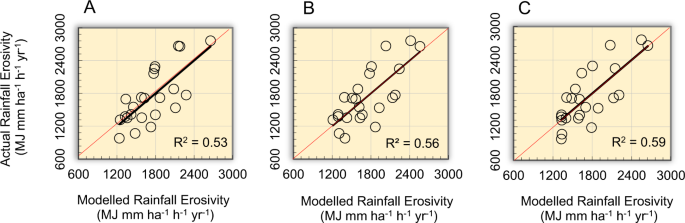
Rainfall erosivity regression model with an annual amount of precipitation (A), linear regression with summer and autumn amount precipitation (B) and multiple linear regression with summer and autumn precipitation (C), versus actual rainfall erosivity.
-
a logarithmic regression: Z = 1974 · LN(Psum + Paut) − 10,877 (Fig. 4B), and
-
a multiple linear regression model: Z = 2.886 · (1.400 · Psum + Paut) − 319 (Fig. 4C),

where Z represents the actual annual rainfall erosivity, Pann the annual precipitation, Psum and Paut, the summer and autumn precipitation, respectively.
The scatter-plots in Fig. 4 present a moderate fitting, with R2 around 0.5–0.6, below the value of 0.74 obtained with the RHEM. Overall, we can conclude that simpler models are less adequate than RHEM to estimate rainfall erosivity. In particular, the insertion of ASSIS(GF) as predictor in Eq. (1) brings a significant improvement in the estimate of annual erosivity, which is difficult to estimate with simpler solutions.
Long-term reconstruction of rainfall erosivity in the PRL
Though consistent with the general trend of actual erosivity data, which are representative of the fluctuations of rainfall erosivity in the PRL, model estimates may not always be adjusted to peaks of erosivity (e.g. high percentiles in Table 1). It can thus be assumed that also in past times high erosivity values may have occurred, which are not entirely captured in the long-term modelled time-series. This may be related to non-linear dynamics implied by the Hurst (H) phenomenon71, i.e. the rate of chaos, with H > 0.5 corresponding to persistent Brownian motions (0.5 corresponding to a random process). The estimated H exponent (R/S method72) equal to 0.84 (above the threshold of 0.65 used by Quian and Rasheed73 to identify a series that can be predicted accurately) reflects the existence of low- and high-intensity storm clusters in the erosivity series, due to the non-linear climate dynamics governing the occurrence of rainfall extremes74. However, the similar distribution and variability to those of the actual data (as identified during the observational period) support the use of model estimates to study trends and fluctuations even though in reality the erosivity peaks may be higher than the modelled ones.
Figure 5 shows the rainfall erosivity evolution over the period 1500–2019 CE. After this reconstruction by means of Eq. (1), the time-series was analysed to find out possible patterns of rainfall aggressiveness and to compare contemporary with historical rainfall erosivity anomalies and their variability. The mean values of rainfall erosivity over the entire series is 1844 CE MJ mm ha−1 h−1 yr−1. Anyhow, the temporal evolution of annual values presents a decreasing trend (Fig. 5A, blue curve and related polynomial), with change points detected in the years 1657 CE (statistics of Buishand75, and Pettitt76) and 1709 CE (statistics of Alexandersson77, and Worsley78), during the grand solar (Maunder) minimum of 1645–1715 CE79. We refer to 1709 CE hereafter, as the starting point of a calmer but more changeable period (Fig. 5A). However, stormy years (with greater erosivity values than the 98th percentile) may occur during any time period.

(A) Timeline evolution of rainfall erosivity reconstructed by Eq. (1) (blue thin curve with signed dates when the 98th percentile is exceeded), and with its 3rd order polynomial regression (blue bold line). Mann–Whitney–Pettit76 statistic (grey curve) with change-point in the year 1709. Variation coefficient running upon 31-year running window (orange thin curve) with related 3rd order polynomial trend (orange bold curve) (B) Wavelet power spectrum with Morlet basis function for the reconstructed rainfall erosivity; bounded colours identify the 0.10 significance level areas; the bell-shaped, black contour marks the limit between the reliable region and the region above the contour where the edge effects occur (arranged from Hammer et al.124).
In this way, the landscape was subject to considerable stress either before or at the start of the Maunder minimum (e.g. 1529, 1579 and 1647 CE) and subsequently (1810, 1976 and 2019 CE; this last with blue dot in Fig. 5A), suggesting that the pressure exerted by aggressive rainfalls can return at periodical intervals. The wavelet power spectrum mostly indicates a ~22-year periodicity (Fig. 5B), which reflects the ~22-year magnetic polarity cycle of sunspot activity80. Similarly, Zanchettin et al.81 found solar-type periodicities, suggesting that the sun may be one of the precursors of hydrological processes in northern Italy, involving the magnetic activity of sunspots.
The periods before and after 1709 CE reveals no similar patterns. Average values indicate that the period 1500–1708 CE, with 2098 MJ mm ha−1 h−1 yr−1, was characterised by more erosive events. The second period, 1709–2019 CE, was instead affected by a less marked regime of erosivity, with 1682 MJ mm ha−1 h−1 yr−1 on average, but accompanied by a more changeable variability pattern (orange curve in Fig. 5A). While a quasi-parallel trend of erosivity (blue bold curve) and coefficient of variation values is visible until 1708 CE, the two curves tend to divergence after this date, the coefficient of variation indicating a kind of exponential growth, passing from 0.20 to 0.35 between 1709 and 2019 CE (orange curve in Fig. 5A).
This means that the PRL has been exposed to progressively increasing inter-annual variability of rainfall erosivity, which translates into greater hazardous landscape stress. As a consequence, disaster-affected areas have become more vulnerable to climate because rainfall aggressiveness has become more changeable. This variability may be caused by different, time-scale-dependent processes (e.g. von Storch and Zwiers82), with erosivity records showing rapid step-like shifts in variability occurring over decadal and multi-decadal time-scales. In particular, extremes may persist and evolve in a more unexpected way. In fact, during recent decades, the aggressiveness seems to indicate a recovery in the erosive activity of rains. This trend is in accordance with a marked increase of erosivity density (the ratio of rainfall erosivity to precipitation, data not shown), which confirms an increased inter-annual variability. Though the frequency of occurrence of daily precipitation was found to decrease over in Italy83, episodes with shorter duration (from 1 to 3 h) have instead enhanced the torrential character of seasonal rains83,84. This accords with what reported by Colarieti Tosti85, which provided sufficient data to show that in the coming decades the polar vortex will undergo a phase of expansion towards the south with consequent exacerbation of the hydrological cycle in the central-western Mediterranean area. Already in 2019, torrential downpours and extreme flooding have battered many parts of Northern Italy, e.g. Venice (northeast) saw record-breaking water levels and the worst flooding in 50 years, and a viaduct near Savona (northwest) was washed away by a mudslide (https://tinyurl.com/tt7apoq).
In northern Italy, short-duration extreme hydrological events have risen over the last 70 years86,87. During 2004–2016, the highest number of such extreme events was mostly recorded in the central Piedmont region88. This trend is in agreement with regional climate simulations predicting increasing precipitation over the high Alpine elevations in the coming decades, associated with increased convective rainfall due to enhanced potential instability by high-elevation surface heating and moistening89. An increase in the frequency of damaging convective weather events over hazard-exposed landscapes is also expected over much of Europe towards the end of the twenty-first century90.
Climate model simulations with the new generation of Coordinated Downscaling Experiment over Europe (EURO-CORDEX91) reveal an increasing trend towards a higher frequency of river floods extremes across most of Europe with future global warming. Towards the end of the twenty-first century, the results from the EURO-CORDEX simulations show no significant change in annual precipitation over northern Italy, but at the same time an approximately 20% increase in maximum daily precipitation92. In order to assess whether there was a change in the frequency distribution, before and after the change-point of 1709 CE, we calculated the frequency histograms pattern for both these periods. It results in that before the change-point (Fig. 6A), the distribution of the erosivity was approximately normal, while later (Fig. 6B), the pattern appears to have a quasi-Poisson distribution.

Frequency distribution of rainfall erosivity for 1500–1708 (A) and 1709–2019 (B).
The mesoscale atmospheric circulation can evolve into landscape-impact weather systems such as rainfall aggressiveness and related damaging hydrological events. We improved the understanding of hydrological extremes, and in turn rainfall erosivity variability, thanks to the long continuous time-series (1500–2019 CE) developed for the PRL from climate records. This was performed with an integrated approach to reconstruct and assess rainfall erosivity for individual years. It included the collection and evaluation of climate documentary sources and a rainfall erosivity model for the reconstruction of past climate erosive variability and detection of climate signals. For the multi-centennial period assessed in this work, the main conclusions can be summarised as follows:
-
1.
Annual rainfall erosivity across the PRL from 1500 CE onwards shows alternate stormy and quiet periods, which may be partially explained by a long-range dependence and non-linear climate dynamics of the pulsed occurrence of rainfall extremes. In this time-scale, a change-point is manifested during the Maunder minimum of solar activity (1645–1715 CE), with remarkable differences before (1500–1708 CE stormy period) and after (1709–2019 CE with a calmer but more changeable period).
-
2.
The generally cold period 1500–1708 CE appears characterised by very stormy years (1529, 1560, 1579, 1610, 1679 and 1703 CE). The following period, until 1809 CE, is a very quiet phase, in the transition to increased storminess activity while inter-annual variability is growing.
-
3.
Since ~1810 rainfall erosivity shows substantially dissimilar dynamics than in the previous periods: precipitation aggressiveness remains quasi-stationary, but some sparse storm erosivity events occur, such as those around the years 1953, 1960, 2001 and, 2014 CE. The way how in the past decades Mediterranean cyclones have been producing trends of rainfall extremes remains elusive93, with significant negative trends of cyclone frequency in spring often compensated by positive trends in summer94. Raible et al.95 supports an increase of extreme cyclone-related precipitation, purely thermodynamically driven by the temperature increase and the Clausius–Clapeyron relation96. An intensification of geo-hydrological hazard owing to an increased occurrence of severe rain events during the past three to five decades is acknowledged for north-western Italy97 and inner hilly areas of central Italy98. However, no sustained long-term trend was observed from 1760 CE over northern Italy (including the Northern Adriatic Sea) in spite of pronounced inter-annual and inter-decadal variability of storminess99.
It can be remarked that the present analysis at an annual scale may mask important variations manifesting at finer time-scales. The methodology applied in this study is, therefore, most appropriate to address inter-annual and inter-decadal time-scales, but does not capture daily to seasonal changes which may impact on hydrology and land conditions and different spatial scales. However, the presented continuous (provisional) rainfall erosivity reconstructions over the PRL are of great importance for all kind of climatic analyses dealing with natural variabilities at decadal and centennial time-scales. They can be used to study the low and high-frequency variability, and the characteristics and extremes of climate at sub-regional scale, and can be compared with model-produced simulations of natural and forced (external and internal) variability for the past centuries. The results also imply that environmental management can use data from long historical time-series as a reference for decision making.
Methods
(R)USLE-based actual rainfall erosivity data
Annual (R)USLE-based rainfall erosivity data (1981–2015) were extracted from a high-resolution database with precipitation measurements taken at 23 locations across the PRL (over 7°–11° E and 44°–46° N), of which 11 are from the upper west side of the Po River Basin (Susa, Luserna, Boves, Mondovì, Bra, Turin, Lanzo, Oropa, Varallo Sesia, Vercelli, and Casale Monferrato, in the Piedmont Region)100, and 12 from the central and lower east-side (Carpeneto, Milano, Zanzarina, Montanaso Lombardo, Colico, Parma, Bedonia, Levanto, Albareto, Piacenza, Brescia and Padua). For the period 1993–2015, (R)USLE-based data were available for the 23 meteorological stations (with updating until 2015)101,102 because the digital National Agrometeorological Network (https://tinyurl.com/h4juzuv) came into operation in 1993. For this period, an annual series of erosivity data for the PRL was obtained by averaging the annual erosivity values determined in each station located in the basin, and this dataset was used to determine model parameters (calibration dataset). Prior to 1993, only data from the western part of the PRL were provided by Piedmont Region stations since 1981100. Such (R)USLE data from the period 1981–1992 were used for an independent evaluation of model estimates (validation dataset). The following adjusted erosivity data—\({\mathrm{AdjR}}({\mathrm{USLE}})_i\)—were obtained from the original R(USLE) data of the set of stations located to the west side of the Po River Basin, which is basically an extrapolation to the whole of the PRL: \({\mathrm{AdjR}}({\mathrm{USLE}})_i = 1646.7\cdot {\mathrm{LN}}\left( {\mathop {\sum}\nolimits_{l = 1}^n {({\mathrm{R}}){\mathrm{USLE}}_i + \overline {P_{{\mathrm{Aut}}_l}} + \overline {P_{{\mathrm{Sut}}_l}} } } \right) - 10,996\), where the actual erosivity data were summed over the n locations (l) and linearly combined with average autumn (\(\overline {P_{{\mathrm{Aut}}_l}}\)) and summer (\(\overline {P_{{\mathrm{Sum}}_l}}\)) precipitation in each year (i). The coefficients of the regression Y = \({\mathrm{AdjR}}({\mathrm{USLE}})_i\) versus X = \({\mathrm{LN}}\left( {\mathop {\sum }\nolimits_{l = 1}^n ({\mathrm{R}}){\mathrm{USLE}}_i + \overline {P_{{\mathrm{Aut}}_l}} + \overline {P_{{\mathrm{Sum}}_l}} } \right)\) were obtained for the period 1993–2015, for which basin-wide (R)USLE data were available (R2 = 0.87).
(R)USLE model103,104 appears in the following form:
where n is the number of recorded years; mj is the number of erosive events during a given month j; k is the index of a kth single event; vr is the rainfall volume (mm) during the rth period of a storm, which splits into m parts; I30 is the maximum 30-min rainfall intensity (mm h−1); ir is the rainfall intensity during the time interval (mm h−1); Pj is the rainfall amount (mm) during a given month j.
Numerical and categorical dependent variables
The reconstruction of annually resolved storm erosivity for the PRL was based on the seasonal precipitation data for a grid covering most of Europe (30W–40°E/30°N–71°N) from 1500 to 2000 on 0.5° by 0.5° resolution105. The CRU Global Climate Dataset106 provides an extension of the seasonal precipitation dataset until 2019. A categorical variable, the annual severity storm index sum (ASSIS), was derived from Diodato et al.56 to overcome the lack of historical information about rain intensity. ASSIS was derived from several sources by transforming documentary information into a record set to 0 (normal event), 1 (stormy event), 2 (very stormy event), 3 (great stormy event) and 4 (extraordinary stormy event).
Historical modelling of rainfall erosivity
For the historical reconstruction of annual rainfall erosivity (MJ mm ha−1 h−1 yr−1), we developed the Rainfall Erosivity Historical Model (REHM), which uses as inputs summer and autumn precipitation data (mm) and Gaussian-filtered values of the reconstructed ASSIS:
where the terms φ and ψ are expressed in mm−1 while the scale parameter A converts the result between brackets in MJ mm ha−1 h−1 yr−1. The process term φ is:
where α (mm−1) and k (mm−1) are empirical parameters. The term φ modulates the autumn erosive precipitation. It equals α when ASSIS(GF) = 0. Since floods occur generally during the autumn season, the Gaussian-filtered annual storm-severity index sum, ASSIS(GF), was selected as an input co-variable to capture storm-energy during this season. The interaction between autumn precipitation and ASSIS(GF) interprets the fact that wet autumn driven by severe storms increases the risk of erosivity. The multiplicative component φ ∙ PAut supports the non-linear dependence of rainfall erosivity on precipitation intensity (e.g. D’Odorico et al.)107. The ASSIS(GF) values from the original ASSIS time-series were smoothed by applying the low-pass Gaussian filtering technique described by Gjelten et al.108. Weighting coefficients (wij) were applied to derive the Gaussian function, ASSIS(GF), for each year j:
where xi is the data point at year i, σ is the standard deviation, and n is the number of years in the series. The series of filtered values is established by letting j run through all data points. To remove variations at shorter time-scales than approximately 10 data points in the time-series, 11-year window (i – j) and σ = 3 years were chosen (e.g. Harris et al.109 and Manara et al.110), which is a way to modulate the impact on rainfall erosivity of the decadal variability and long-term trend of storm-severity. Summer precipitation is characterised by an intrinsic high variability. The intensity of summer rainfall is modulated by Eq. (4), a modified version of the variation coefficient developed by Aronica and Ferro111:
where SD is the inter-seasonal standard deviation and Max(Ps) is the maximum seasonal precipitation per year (mm). Winter and spring rainfalls have not been taken into account by the model because rainfall intensity is generally low in those seasons in northern Italy, with limited erosive force. The concept of the model is summarised in Fig. 7 following Diodato and Bellocchi112. It shows that in Northern Italy brief and intense convective storms are more common in summer while autumn rains (of long duration and low intensity) usually originate from broad mid-latitude frontal activity. They carry high volumes of rainwater thanks to orographically enhanced stratiform precipitation (expressed by high percentiles), which also cause large-scale hydrological processes like flooding113. These processes are captured in the Rainfall Erosivity Historical Model by the storm-severity index of Eq. (2). Highly intensive convective rainfall results instead in the splash-erosivity process interpreted by the variation coefficient of Eq. (4). In this case, raindrops with high kinetic energy may cause the local detachment of soil particles114.

To assess the model, statistical analyses were performed with STATGRAPHICS115, with the graphical support of WESSA116 and CurveExpert routines117. The mean absolute error (MAE, MJ mm ha−1 h−1 yr−1) was used to quantify the differences between actual and predicted erosivity values, while determination coefficient (0 ≤ R2 ≤ 1, optimum) and slope (b = 1, optimum) assessed the linear relationship between the two series. The Kling–Gupta index (−∞ < KGE ≤ 1118) was used as an efficiency measure, with KGE > −0.41 indicating that a model improves upon the means of observations as a benchmark predictor119. The Durbin–Watson statistic120,121 was performed to test for auto-correlated residuals because large temporal dependence may induce spurious correlations122. ANOVA p-values were used to present the statistical significance of the regression between estimates and the actual data. Student t-test and Kolmogorov–Smirnov test were applied to determine whether the two groups (estimates and actual data) originate from the same population. The variance ratio F-test was used to test the difference between variances.
Data availability
The full set data are available in a data file published along with this article.
Change history
18 February 2021
A Correction to this paper has been published: https://doi.org/10.1038/s41612-021-00164-z
References
Sabatier, P., Dezileau, L., Colin, C. & Briqueu, L. 7000 years of paleostorm activity in the NW Mediterranean Sea in response to Holocene climate events. Quat. Res. 77, 1–11 (2012).
Benito, G. et al. Recurring flood distribution patterns related to short-term Holocene climatic variability. Sci. Rep. 5, 16398 (2015).
Tippett, M. K. Extreme weather and climate. npj Clim. Atmos. Sci. 1, 45 (2018).
Goslin, J. et al. Holocene centennial to millennial shift in North-Atlantic storminess and ocean dynamics. Sci. Rep. 8, 12778 (2018).
Thomas, M. F. Landscape sensitivity in time and space – an introduction. Catena 42, 83–98 (2001).
Phillips, J. D. Evolutionary geomorphology: thresholds and nonlinearity in landform response to environmental change. Hydrol. Earth Syst. Sci. 10, 731–742 (2006).
Baynes, E. R. C. et al. River self-organisation inhibits discharge control on waterfall migration. Sci. Rep. 8, 2444 (2015).
Wei, W., Chen, L., Fu, B., Lü, Y. & Gong, J. Responses of water erosion to rainfall extremes and vegetation types in a loess semiarid hilly area, NW China. Hydrol. Process. 23, 1780–1791 (2009).
Knapp, A. K. et al. Consequences of more extreme precipitation regimes for terrestrial ecosystems. BioScience 58, 811–821 (2008).
AghaKouchak, A. et al. How do natural hazards cascade to cause disasters? Nature 561, 458–460 (2018).
Toy, T. J., Foster, G. R. & Renard, K. G. Soil Erosion: Prediction, Measurement, and Control (John Wiley & Sons, New York, 2002).
Schmidt, S., Alewell, C., Panagos, P. & Meusburger, K. Regionalization of monthly rainfall erosivity patterns in Switzerland. Hydrol. Earth Syst. Sci. 20, 4359–4373 (2016).
Lamoureux, S. Temporal patterns of suspended sediment yield following moderate to extreme hydrological events recorded in varved lacustrine sediments. Earth Surf. Process. Landf. 27, 1107–1124 (2002).
Marinova, E., Kirleis, W. & Bittmann, F. Human landscapes and climate change during the Holocene. Veg. Hist. Archaeobot. 21, 245–248 (2012).
Donat, M. G., Lowry, A. L., Alexander, L. V., O’Gorman, P. A. & Maher, N. More extreme precipitation in the world’s dry and wet regions. Nat. Clim. Change 6, 508–514 (2016).
De Luca, P., Messori, G., Wilby, R. L., Mazzoleni, M. & Di Baldassarre, G. Concurrent wet and dry hydrological extremes at the global scale. Earth Syst. Dynam. 11, 251–266 (2020).
Schulte, L., Schillereff, D. & Santisteban, J. I. Pluridisciplinary analysis and multi-archive reconstruction of paleofloods: societal demand, challenges and progress. Glob. Planet. Change 177, 225–238 (2019).
Gelagay, H. S. & Minale, A. S. Soil loss estimation using GIS and remote sensing techniques: a case of Koga watershed. Northwest. Ethiop. Int. Soil Water Conserv. Res. 4, 126–136 (2016).
Borrelli, P. et al. An assessment of the global impact of 21st century land use change on soil erosion. Nat. Commun. 8, 2013 (2017).
Papathoma, M. & Dominey-Howes, D. Tsunami vulnerability assessment and its implications for coastal hazard analysis and disaster management planning, Gulf of Corinth. Greece Nat. Hazard. Earth Syst. Sci. 3, 733–747 (2003).
Burt, T., Boardman, J., Foster, I. & Howden, N. More rain, less soil: long-term changes in rainfall intensity with climate change. Earth Surf. Process. Landf. 41, 563–566 (2016).
Hoeppe, P. Trends in weather related disasters – consequences for insurers and society. Weather Clim. Extremes 11, 70–79 (2016).
Panagos, P. et al. Cost of agricultural productivity loss due to soil erosion in the European Union: from direct cost evaluation approaches to the use of macroeconomic models. Land Degrad. Dev. 29, 471–484 (2018).
Giorgi, F., Coppola, E. & Raffaele, F. Threatening levels of cumulative stress due to hydroclimatic extremes in the 21st century. npj Clim. Atmos. Sci. 1, 18 (2018).
Trenberth, K. E. et al. Global warming and changes in drought. Nat. Clim. Change 4, 17–22 (2014).
Zhang, X., Zwiers, F. W., Li, G., Wan, H. & Cannon, A. J. Complexity in estimating past and future extreme short-duration rainfall. Nat. Geosci. 10, 255–259 (2017).
Prein, A. F. & Pendergrass, A. G. Can we constrain uncertainty in hydrologic cycle projections? Geophys. Res. Lett. 46, 3911–3916 (2019).
Lenderink, G. & van Meijgaard, E. Increase in hourly precipitation extremes beyond expectations from temperature changes. Nat. Geosci. 1, 511–514 (2008).
Berg, P., Moseley, C. & Haerter, J. O. Strong increase in convective precipitation in response to higher temperatures. Nat. Geosci. 6, 181–185 (2013).
Yin, J. et al. Large increase in global storm runoff extremes driven by climate and anthropogenic changes. Nat. Commun. 9, 4389 (2018).
Johnstone, J. F. et al. Changing disturbance regimes, ecological memory, and forest resilience. Front. Ecol. Environ. 14, 369–378 (2016).
Hughes, T. P. et al. Ecological memory modifies the cumulative impact of recurrent climate extremes. Nat. Clim. Chang. 9, 40–43 (2019).
Sauerborn, P., Klein, A., Botschek, J. & Skowronek, A. Future rainfall erosivity derived from large-scale climate models – methods and scenarios for a humid region. Geoderma 93, 269–276 (1999).
Allen, M. R. & Ingram, W. J. Constraints on future changes in climate and the hydrologic cycle. Nature 419, 224–232 (2002).
Diodato, N., Bellocchi, G., Chirico, G. B. & Romano, N. How the aggressiveness of rainfalls in the Mediterranean lands is enhanced by climate change. Clim. Change 108, 591–599 (2011).
Polade, S. D., Pierce, D. W., Cayan, D., Gershunov, A. & Dettinger, M. D. The key role of dry days in changing regional climate and precipitation regimes. Sci. Rep. 4, 4364 (2014).
Le Bissonnais, Y., Montier, C., Jamagne, M., Daroussin, J. & King, D. Mapping erosion risk for cultivated soil in France. Catena 46, 207–220 (2002).
Longman, J., Veres, D., Ersek, V., Haliuc, A. & Wennrich, V. Runoff events and related rainfall variability in the Southern Carpathians during the last 2000 years. Sci. Rep. 9, 5334 (2019).
Blenkinsop, S. et al. The INTENSE project: using observations and models to understand the past, present and future of sub-daily rainfall extremes. Adv. Sci. Res. 15, 117–126 (2018).
Koutsoyiannis, D. & A. Langousis. Treatise on Water Science (ed. P. Wilderer, P. & Uhlenbrook, S.) Ch. 2, 27–78 (Academic Press, Oxford, 2011).
Koutsoyiannis, D., Dimitriadis, P., Lombardo, F., & Stevens, S. Advances in Nonlinear Geosciences (ed. Tsonis A.) 237–278 (Springer, Cham, 2018).
Glur, L. et al. Frequent floods in the European Alps coincide with cooler periods of the past 2500 years. Sci. Rep. 3, 2770 (2013).
Schulte, L. et al. A 2600-year history of floods in the Bernese Alps, Switzerland: frequencies, mechanisms and climate forcing. Hydrol. Earth Syst. Sci. 19, 3047–3072 (2015).
Diodato, N. et al. Historical evolution of slope instability in the Calore River Basin. South. Italy Geomorphol. 282, 74–84 (2017).
Iliopoulou, T. & Koutsoyiannis, D. Projecting the future of rainfall extremes: better classic than trendy. J. Hydrol. 588, https://doi.org/10.1016/j.jhydrol.2020.125005 (2020).
Ljungqvist, F. C. et al. Northern Hemisphere hydroclimate variability over the past twelve centuries. Nature 532, 94–98 (2016).
Ljungqvist, F. C. et al. European warm-season temperature and hydroclimate since 850 CE. Environ. Res. Lett. 14, 084015 (2019).
Xie, S.-P. et al. Towards predictive understanding of regional climate change. Nat. Clim. Change 5, 921–930 (2015).
Boorman, D. B. & Sefton, C. E. M. Recognising the uncertainty in the quantification of the effects of climate change on hydrological response. Clim. Change 35, 415–434 (1997).
Goosse, H., Renssen, H., Timmermann, A. & Raymond, S. B. Internal and forced climate variability during the last millennium: a model-data comparison using ensemble simulations. Quat. Sci. Rev. 24, 1345–1360 (2005).
Dimitriadis, P. & Koutsoyiannis, D. Stochastic synthesis approximating any process dependence and distribution. Stoch. Environ. Res. Risk Assess. 32, 1493–1515 (2018).
Blöchl, G. et al. At what scales do climate variability and land cover change impact on flooding and low flows? Hydrol. Process. 21, 1241–1247 (2007).
Pichard, G., Arnaud-Fassetta, G., Moron, V. & Roucaute, E. Hydro-climatology of the Lower Rhône Valley: historical flood reconstruction (AD 1300–2000) based on documentary and instrumental sources. Hydrol. Sci. J. 62, 1772–1795 (2017).
Benito, G., Macklin, M. G., Zielhofer, C., Jones, A. F. & Machado, M. J. Holocene flooding and climate change in the Mediterranean. Catena 130, 13–33 (2015).
Corella, J. P., Valero-Garcés, P. L., Vicente-Serrano, S. M., Brauer, A. & Benito, G. Three millennia of heavy rainfalls in Western Mediterranean: frequency, seasonality and atmospheric drivers. Sci. Rep. 6, 38206 (2016).
Diodato, N., Ljungqvist, F. C. & Bellocchi, G. A millennium-long reconstruction of damaging hydrological events across Italy. Sci. Rep. 9, 9963 (2019).
Allan, R. et al. Toward integrated historical climate research: the example of atmospheric circulation reconstructions over the Earth. Wiley Interdiscip. Rev. Clim. Change 7, 164–174 (2016).
Krishnaswamy, J., Lavine, M., Richter, D. D. & Korfmacher, K. Dynamic modeling of long-term sedimentation in the Yadkin River basin. Adv. Water Resour. 23, 881–892 (2000).
Luino, F. L’Italia dei disastri, dati e riflessioni sull’impatto degli eventi naturali 1861–2013 (Bononia University Press, Bologna, 2013) [in Italian].
Lanzani, G. Il Bacino Padano: un caso Europeo. Ecoscienza. https://www.arpae.it/cms3/documenti/_cerca_doc/ecoscienza/ecoscienza2017_1/lanzani_es2017_01.pdf (2017) [in Italian].
Cati, L. Idrografia e idrologia del Po. Pubblicazione n. 19 dell’Ufficio Idrografico del Po (Istituto Poligrafico e Zecca dello Stato, Rome, 1981) [in Italian].
Franco, A. A probabilistic approach to classify the levee reliability. MS thesis, University of Bologna, https://amslaurea.unibo.it/10120/# (2016).
Strahler, A. H. & Strahler, A. Introducing Physical Geography 2nd edn. (John Wiley & Sons, Hoboken NJ, 2000).
Renard, K. G., Foster, G. R., Weesies, G. A., McCool, D. K. & Yoder, D. C. Predicting Soil Erosion by Water: A Guide to Conservation Planning with the Revised Universal Soil Loss Equation (RUSLE) (USDA-ARS Agriculture Handbook No. 703, Washington DC, 1997).
Wischmeier, W. H. & Smith, D. D. Predicting Rainfall Erosion Losses. A Guide to Conservation Planning (USDA-ARS Agriculture Handbook No. 537, Washington DC, 1978).
Poirier, C., Poitevin, C. & Chaumillon, E. Comparison of estuarine sediment record with modelled rates of sediment supply from a western European catchment since 1500. C. R. Geosci. 348, 479–488 (2016).
Diodato, N., Borrelli, P., Fiener, P., Bellocchi, G. & Romano, N. Discovering historical rainfall erosivity with a parsimonious approach: A case study in Western Germany. J. Hydrol. 544, 1–9 (2017).
Diodato, N., Ceccarelli, M. & Bellocchi, G. Decadal and century-long changes in the reconstruction of erosive rainfall anomalies at a Mediterranean fluvial basin. Earth Surf. Process. Landf. 33, 2078–2093 (2008).
Pinto J. G., Klawa, M., Ulbrich, U., Rudari, R. & Speth, P. Extreme precipitation events over north-west Italy and their relationship with tropical–extratropical interactions over the Atlantic. In Proc. Third EGS Plinius Conference on Mediterranean Storms, Baja Sardinia 321–332 (2001).
Diodato, N., Ljungqvist, F. C. & Bellocchi, G. Monthly storminess over the Po River Basin during the past millennium (800–2018 CE). Environ. Res. Commun. 2, 031004 (2020).
Hurst, H. E. Long term storage capacity of reservoirs. Trans. ASCE 116, 776–808 (1951).
Jens, F. Fractals (Plenum Press, New York, NY, USA, 1988).
Quian, B. & Rasheed, K. Hurst exponent and financial market predictability. In Proc. 2nd IASTED International Conference on Financial Engineering and Applications, Cambridge, MA, USA, 8–11 November 2004 203–209 (2004).
Tyralis, H. et al. On the long-range dependence properties of annual precipitation using a global network of instrumental measurements. Adv. Water Resour. 111, 301–318 (2018).
Reinard, K. G. & Freimund, J. R. Using monthly precipitation data to estimate the R-factor in the revised USLE. J. Hydrol. 157, 287–306 (1994).
Buishand, T. A. Some methods for testing the homogeneity of rainfall records. J. Hydrol. 58, 11–27 (1982).
Pettitt, A. N. A non-parametric approach to the change-point detection. Appl. Stat. 28, 126–135 (1979).
Alexandersson, H. A homogeneity test applied to precipitation data. J. Climatol. 6, 661–675 (1986).
Worsley, K. J. Testing for a two-phase multiple regression. Technometrics 25, 35–42 (1983).
Eddy, J. A. The Maunder minimum. Science 192, 1189–1202 (1976).
Hale, G. E., Ellerman, F., Nicholson, S. B. & Joy, A. H. The magnetic polarity of sunspots. Astrophys. J. 49, 153–178 (1919).
Zanchettin, D., Rubino, A., Traverso, P. & Tomasino, M. Impact of variations in solar activity on hydrological decadal patterns in northern Italy. J. Geophys. Res. 113, D12102 (2008).
von Storch, H. & Zwiers, F. W. Statistical Analysis in Climate Research (Cambridge University Press, Cambridge, 1999).
Cislaghi, M., De Michele, C., Ghezzi, A. & Rosso, R. Statistical assessment of trends and oscillations in rainfall dynamics: analysis of long daily Italian series. Atmos. Res. 77, 188–202 (2005).
Pavan, V., Tomozeiu, R., Cacciamani, C. & Di Lorenzo, M. Daily precipitation observations over Emilia-Romagna: mean values and extremes. Int. J. Climatol. 28, 2065–2079 (2008).
Colarieti Tosti, C. Il clima del futuro? La chiave è nel passato. https://tinyurl.com/u5hp3w6 (2014) [in Italian].
Saidi, H., Ciampittiello, M., Dresti, C. & Ghiglieri, G. Assessment of trends in extreme precipitation events: a case study in Piedmont (North-West Italy). Water Resour. Manag. 29, 63–80 (2015).
Faccini, F. et al. Role of rainfall intensity and urban sprawl in the 2014 flash flood in Genoa City, Bisagno catchment (Liguria, Italy). Appl. Geogr. 98, 224–241 (2018).
Baronetti, A., Acquaotta, F. & Fratianni, S. Rainfall variability from a dense rain gauge network in North-West Italy. Clim. Res. 75, 201–213 (2018).
Giorgi, F. et al. Enhanced summer convective rainfall at Alpine high elevations in response to climate warming. Nat. Geosci. 9, 584–589 (2016).
Rädler, A. T., Groenemeijer, P. H., Faust, E., Sausen, R. & Púčik, T. Frequency of severe thunderstorms across Europe expected to increase in the 21st century due to rising instability. npj Clim. Atmos. Sci. 2, 30 (2019).
Jacob, D. et al. EURO-CORDEX: new high-resolution climate change projections for European impact research. Reg. Environ. Change 14, 563–578 (2014).
Alfieri, L., Burek, P., Feyen, L. & Forzieri, G. Global warming increases the frequency of river floods in Europe. Hydrol. Earth Syst. Sci. 19, 2247–2260 (2015).
Lionello, P. et al. in Mediterranean Climate Variability (eds Lionello, P., Malanotte-Rizzoli, P. & Boscolo, R.) 1–26 (Elsevier, Amsterdam, 2006).
Lionello, P. et al. Objective climatology of cyclones in the Mediterranean region: a consensus view among methods with different system identification and tracking criteria. Tellus 68A, 29391 (2016).
Raible, C. C., Messmer, M., Lehner, F., Stocker, T. F. & Blender, R. Extratropical cyclone statistics during the last millennium and the 21st century. Climate 14, 1499–1514 (2018).
Kirby, M. E. Water’s past revisited to predict its future. Nature 532, 44–45 (2016).
Paliaga, G., Luino, F., Turconi, L., De Graff, J. V. & Faccini, F. Terraced landscapes on Portofino promontory (Italy): Identification, geo-hydrological hazard and management. Water 12, 435 (2020).
Pieri, C., Rondini, D. & Ventura, F. Changes in the rainfall – streamflow regimes related to climate change in a small catchment in Northern Italy. Theor. Appl. Climatol. 129, 1075–1087 (2016).
Matulla, C. et al. Storminess in northern Italy and the Adriatic Sea reaching back to 1760. Phys. Chem. Earth 40–41, 80–85 (2012).
Acquaotta, F., Baronetti, A., Bentivenga, M., Fratianni, S. & Piccarreta, M. Estimation of rainfall erosivity in piedmont (Northwestern Italy) by using 10-minute fixed-interval rainfall data. Idojaras 12, 1–18 (2019).
Diodato, N. Predicting RUSLE (Revised Universal Soil Loss Equation) monthly erosivity index from readily available rainfall data in Mediterranean area. Environmentalist 26, 63–70 (2006).
Renard, K. G., Yoder, D. C., Ligtle, D. T., & Darney S. M. in Handbook of Erosion Modelling (eds Morgan, R. P. C. & Nearing, M. A.) 153–170 (Wiley-Blackwell, Oxford, 2011).
Diodato, N. & Bellocchi, G. MedREM, a rainfall erosivity model for the Mediterranean region. J. Hydrol. 387, 119–127 (2010).
Pauling, A., Luterbacher, J. & Wanner, H. Evaluation of proxies for European and North Atlantic temperature field reconstructions. Geophys. Res. Lett. 30, 1787 (2003).
Jones, P. D. & Harris, I. C. Climatic Research Unit (CRU): Time-series (TS) Datasets of Variations in Climate with Variations in Other Phenomena v3. NCAS British Atmospheric Data Centre. http://catalogue.ceda.ac.uk/uuid/3f8944800cc48e1cbc29a5ee12d8542d (2008).
D’Odorico, P., Yoo, J. & Over, T. M. An assessment of ENSO-induced patterns of rainfall erosivity in the Southwestern United States. J. Clim. 14, 4230–4242 (2001).
Gjelten, H. M. et al. Air temperature variations and gradients along the coast and fjords of western Spitsbergen. Polar Res. 35, 29878 (2016).
Harris, C. et al. Warming permafrost in European mountains. Glob. Planet. Change 39, 215–225 (2003).
Manara, V. et al. Detection of dimming/brightening in Italy from homogenized all-sky and clear-sky surface solar radiation records and underlying causes (1959–2013). Atmos. Chem. Phys. 16, 11145–11161 (2016).
Aronica, G. & Ferro, V. Rainfall erosivity over the Calabrian region. Hydrol. Sci. J. 42, 35–48 (1997).
Diodato, N. & Bellocchi, G. Storminess and Environmental Change (Springer, Dordrecht, 2014).
Van Delden, A. The synoptic setting of thunderstorms in western Europe. Atmos. Res. 56, 89–110 (2001).
Kinnell, P. I. A. The problem of assessing the erosive power of rainfall from meteorological observations. Soil Sci. Soc. Am. J. 37, 617–621 (1973).
Nau, R. STATGRAPHICS V.5: Overview & Tutorial Guide. http://www.duke.edu/~rnau/sgwin5.pdf (2005).
Wessa, P. Free Statistics Software, Office for Research Development and Education, version 1.2.1. https://www.wessa.net (2019).
Hyams, D. G. CurveExpert Professional Documentation Release 2.6.5 https://docs.curveexpert.net/curveexpert/pro/_static/CurveExpertPro.pdf (2018).
Kling, H., Fuchs, M. & Paulin, M. Runoff conditions in the upper Danube basin under an ensemble of climate change scenarios. J. Hydrol. 424–425, 264–277 (2012).
Knoben, W. J. M., Freer, J. E. & Woods, R. A. Technical note: Inherent benchmark or not? Comparing Nash–Sutcliffe and Kling-Gupta efficiency scores. Hydrol. Earth Syst. Sci. 23, 4323–4331 (2019).
Durbin, J. & Watson, G. S. Testing for serial correlation in least squares regression, I. Biometrika 37, 409–428 (1950).
Durbin, J. & Watson, G. S. Testing for serial correlation in least squares regression, II. Biometrika 38, 159–179 (1951).
Granger, C. W. J., Hyung, N. & Jeon, Y. Spurious regressions with stationary series. Appl. Econ. 33, 899–904 (2001).
Panagos, P. et al. Global rainfall erosivity assessment based on high-temporal resolution rainfall records. Sci. Rep. 7, 4175 (2017).
Hammer, Ø., Harper, D. A. T. & Ryan, P. D. Past: paleontological statistics software package for education and data analysis. Palaeontol. Electr. https://palaeo-electronica.org/2001_1/past/past.pdf (2001).
Gaume, E. et al. A compilation of data on European flash floods. J. Hydrol. 367, 70–78 (2009).
Acknowledgements
F.C.L. was supported by the Swedish Research Council (Vetenskapsrådet, Grant No. 2018-01272), and conducted most of the work with this article as a Pro Futura Scientia XIII Fellow funded by the Swedish Collegium for Advanced Study through Riksbankens Jubileumsfond.
Funding
Open Access funding provided by Stockholm University.
Author information
Authors and Affiliations
Contributions
N.D. and G.B. developed the original research design and collected and analysed the historical documentary data. N.D., F.C.L. and G.B. wrote the article together and made the interpretations together. All authors reviewed the final manuscript.
Corresponding author
Ethics declarations
Competing interests
The authors declare no competing interests.
Additional information
Publisher’s note Springer Nature remains neutral with regard to jurisdictional claims in published maps and institutional affiliations.
Supplementary information
Rights and permissions
Open Access This article is licensed under a Creative Commons Attribution 4.0 International License, which permits use, sharing, adaptation, distribution and reproduction in any medium or format, as long as you give appropriate credit to the original author(s) and the source, provide a link to the Creative Commons license, and indicate if changes were made. The images or other third party material in this article are included in the article’s Creative Commons license, unless indicated otherwise in a credit line to the material. If material is not included in the article’s Creative Commons license and your intended use is not permitted by statutory regulation or exceeds the permitted use, you will need to obtain permission directly from the copyright holder. To view a copy of this license, visit http://creativecommons.org/licenses/by/4.0/.
About this article

Cite this article
Diodato, N., Ljungqvist, F.C. & Bellocchi, G. Historical predictability of rainfall erosivity: a reconstruction for monitoring extremes over Northern Italy (1500–2019). npj Clim Atmos Sci 3, 46 (2020). https://doi.org/10.1038/s41612-020-00144-9
Received:
Accepted:
Published:
DOI: https://doi.org/10.1038/s41612-020-00144-9
